INTERSPEECH 2016 September 8–12, 2016, San Francisco, USA
A DNN-HMM Approach to Story Segmentation Jia Yu1 , Xiong Xiao2 , Lei Xie1 , Eng Siong Chng2,3 , Haizhou Li2,3,4 1
Shaanxi Provincial Key Laboratory of Speech and Image Information Processing, School of Computer Science, Northwestern Polytechnical University, Xi’an, China 2 Temasek Laboratories@NTU, Nanyang Technological University, Singapore 3 School of Computer Engineering, Nanyang Technological University, Singapore 4 Institute for Infocomm Research, A*STAR, Singapore {jiayu,lxie}@nwpu-aslp.org, {xiaoxiong,ASESChng}@ntu.edu.sg,
[email protected]
Abstract
ing is one of the methods focusing on identifying boundaries through local lexical comparison, while other lexical methods aims to find an optimal segmentation under some global criteria [22, 23]. Popular approaches include dynamic programing (DP) [22, 23, 24], Ncuts [25], BayesSeg [26] and dd-CRP [27]. The lexical cohesion based approaches mentioned above mostly rely on the tf-idf representation of a sentence, which is not necessarily attached to topics of stories. Instead, probabilistic topic models, e.g., probabilistic latent semantic analysis (pLSA) [28], latent Dirichlet allocation (LDA) [29] and LapPLSA [28], learn from a training corpus, to map a tf-idf representation to a topic representation [25]. These generative topic models assume documents are comprised of topics following certain distributions and words are generated from these topics. Significant performance improvements have been observed when a tf-idf representation is substituted by a topic representation in both TextTiling and DP approaches [30, 31]. As another generative model, hidden Markov model (HMM) [32] has been successfully introduced to automatically infer story boundaries [15, 16, 14]. A story is treated as an instance of an underlying topic (a hidden state) and words are generated from the distribution of the topic. The transition from one topic to another indicates a story boundary. Transition and emission probabilities of the hidden states can be inferred from a training corpus. Specifically, the emission probability of a state is inferred by a topic-dependent language model (LM), which is calculated by word counting. In the decoding process, the Viterbi algorithm is used to label the input sequences. The position of topic change is regarded as a story boundary. In this paper, we introduce the DNN-HMM hybrid model to the story segmentation task. Unlike the topic-dependent LM used in traditional HMM-based approach [15, 16, 14], which is a generative model of the word sequence, we use a DNN to directly map the word observation into topic posterior probabilities. The input features of the DNN is the BOW computed from a local context of every candidate story boundary. DNN is known to be able to learn meaningful continuous features for words and hence has better discriminative and generalization capability than n-gram models [33, 34].
Hidden Markov model (HMM) is one of the popular techniques for story segmentation, where hidden Markov states represent the topics, and the emission distributions of n-gram language model (LM) are dependent on the states. Given a text document, a Viterbi decoder finds the hidden story sequence, with a change of topic indicating a story boundary. In this paper, we propose a discriminative approach to story boundary detection. In the HMM framework, we use deep neural network (DNN) to estimate the posterior probability of topics given the bag-ofwords in the local context. We call it the DNN-HMM approach. We consider the topic dependent LM as a generative modeling technique, and the DNN-HMM as the discriminative solution. Experiments on topic detection and tracking (TDT2) task show that DNN-HMM outperforms traditional n-gram LM approach significantly and achieves state-of-the-art performance. Index Terms: Deep neural network, Hidden Markov Model, story segmentation
1. Introduction Story segmentation is a task to partition a stream of text, audio or video into a sequence of topically coherent segments named as stories [1, 2, 3, 4]. The task serves as a necessary precursor for subsequent tasks such as topic detection and tracking [1, 5], summarization [6], information extraction [7], indexing and retrieval [8]. Automatic story segmentation has gained ever-increasingly interests with the explosive growth of multimedia data. Specifically, this paper addresses the task of segmenting a speech recognition transcript (i.e., from broadcast news) to a sequence of stories by a hybrid deep neural network (DNN) - hidden Markov model (HMM) approach that has achieved tremendous success in speech recognition [9]. Story segmentation has been historically studied through different media types (audio/prosodic [10, 11, 12], video [13] and text [14, 2, 15, 16, 4, 17]) and genres (broadcast news [18], meeting recordings [17] and lectures [19, 10]). With recent progress in large vocabulary continuous speech recognition (LVCSR), lexical cohesion based methods have drawn much attention for story segmentation of spoken documents [4, 20, 21]. These methods work on a sequence of words and reveal story transitions that manifest semantic topic shifts. As one of the earliest approaches, TextTiling [4, 20] measures the lexical similarity (i.e. via cosine) between adjacent sentences and story boundaries are discovered at the local similarity minima, where sentences are represented by bag-of-words (BOW) or term frequency – inverted document frequency (tf-idf ) vectors. TextTil-
Copyright © 2016 ISCA
2. DNN-HMM Model for Story Segmentation Fig. 1 depicts the architecture of the proposed DNN-HMM approach for story segmentation. Each HMM state represents a topic and a transition matrix is used to model the probabilities of switching between stories. The DNN produces topic posteri-
1527
http://dx.doi.org/10.21437/Interspeech.2016-873
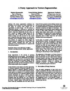
Figure 2: Predicted topic posterior probabilities versus true topic label. Darker means higher probability. (a) is the topic posteriors of words predicted by DNN with BOW input. (b) is the true topic class label of the words. The data used to generate the plot are stories taken from TDT2 corpus.
Figure 1: The DNN-HMM approach for story segmentation.
independent given the state sequence, hence
or probabilities given the BOW computed from the local context of candidate story boundaries. The posterior is converted to the likelihood score for Viterbi decoding (i.e. the emission probability of the states) using the Bayesian rule in a similar way as in the DNN-HMM acoustic model for speech recognition [9].
p(w|z) =
arg max p(z|w; θ) z
(1)
where w = [w1 , ..., wT ] is a sequence of T words observed, z = [z1 , ..., zT ] is the topic sequence to be inferred, and θ represent the HMM parameters including the transition probabilities and the state emission PDFs. Here we assume that each word is an observation. By applying the Bayesian’s rule, the above optimization problem is equivalent to: ˆ z
=
arg max p(w|z; θ)p(z)/p(w)
(2)
=
arg max p(w|z; θ)p(z)
(3)
z
z
2.2. DNN based Topic Posterior Prediction A DNN is actually a multi-layer perception (MLP), i.e., a feedforward neural network model that maps sets of input data onto a set of outputs. It can be considered as a hierarchical feature learner with a nonlinear transformation refining the input representation to a better one, which is topic posterior in our case. As different topics usually have different word distributions, the input of DNN at word wt is the BOW computed from the local context of the current word, defined by
where p(w) does not depend on z and hence ignored in the optimization problem. p(z) is the transition probabilities between states p(z) = p(z1 )
T ∏
p(zt |zt−1 )
(5)
where p(wt |zt ) is the conditional distribution of the word given the topic, i.e. topic-dependent LM. Note that the formulation in (5) only allows unigram topic LM to be used. To use higher order ngram for topic LM, we can use a fixed window of words [35] or sentence [15] as the basic observation unit. The topic-dependent LM and state transition probabilities can be trained from a set of text documents, with story boundary and topic label annotated. If the topic label is not available, we can cluster the segmented stories into a set of topics. With these models and the definition of the optimization problem from (3) to (5), we can use the Viterbi algorithm [36] to find the optimal topic sequence for test data efficiently. The HMM approach to story segmentation is a generative approach, i.e. it models the generation process of the stories and words, and reverse the generative process at test phase to infer the topic sequence. Motivated by the recent success of DNN-HMM approach in ASR, we propose to use a discriminative approach for the story segmentation task. Specifically, we propose to replace the topic-dependent LM with a DNN that predicts the posterior probabilities of the topics directly given a window of observed words.
HMM is a generative model for sequence data and has been applied to the text segmentation task [14]. An HMM contains a set of N states, each representing a topic. The transition between the states can be modeled by a N × N matrix, which can be learnt from segmented and labeled training data. Each state is associated with an emission probability distribution function (PDF) that models the n-gram word distribution for the topic represented by the state. For example, in [15], a topic-dependent unigram language model is used as the emission probability of each HMM state. Given a sequence of words and the trained HMM, we can infer the topic sequence by solving the following optimization problem: =
p(wt |zt )
t=1
2.1. HMM based Story Segmentation
ˆ z
T ∏
1 xt = ′ T +1
(4)
t=2
where p(zt |zt−1 ) is the transition probability from state zt−1 to zt . The words in neighboring time steps are assumed to be
T ′ /2
∑
w ˜t−τ
(6)
τ =−T ′ /2
where w ˜t is the 1-hot vector representation of the word wt , and T ′ + 1 is the context window size. At the beginning and end-
1528
6
(2) (2) (1) (1) (1) (2)
8
(2)
7 9
(2)
Cluster Index
5
(2)
0 1 2 3 4
(2)
ing of the input word sequence, we won’t be able to get the full context, and the normalization term T ′ + 1 is replaced by the actual number of words used in the sum. In this way, we normalize xt independent of its position in the input sequence. The BOW vector xt is sparse and has a dimension of |V |, i.e. the size of the vocabulary. It captures the unigram statistics around the current word wt , and hence contains information to predict the topic class for wt . The BOW feature vector is nonlinearly transformed by the DNN to generate the topic posteriors. The hidden layers of the DNN produces their output as follows:
01077 01007 01059 01303 01252 00902 00891 00962 00644 00587 00816 00800 00794 01390 01226 00555 01244 01235 00691 00712 01424 01413 01448 01408 01404 00408 00379 00186 00188 00069 00026 00101 00236 00213 00242 00309 00320 01145 01137 01179 00523 00498 00467 00443 00489 00525 00477 01115 01106 01127 01123 01119
Word ID
hl = fl (Wl hl−1 + bl )
(7) Figure 3: The distribution of most frequent words in 10 clusters. X-axis is the index of frequent words in the 10 clusters, while y-axis is the index of clusters. Darker color means higher probability of occurrence.
where hl , fl , Wl , and bl are the output, activation function, transform matrix, and bias vector at layer l, respectively. In this study, we use the sigmoid activation function for hidden layers. Note that the input of the first hidden layer h0 = xt . The posterior probability of the ith topics given the input is ehL (i) p(zt = i|xt ) = ∑J hL (j) j=1 e
3. Experiments 3.1. Experimental Setup
(8)
We carried out experiments on Topic Detection and Tracking (TDT2) [5] corpus, which contains 2,280 English broadcast news programs. Our testing set includes 240 programs, chosen as subset of the whole corpus, with the remaining 1,800 programs as training set and 240 programs as development set. All texts were preprocessed by a Porter stemmer and stop words were removed. The size of vocabulary is 57,817. In the test set, each of the out-of-vocabulary words is replaced by its prior word. In the unsupervised clustering process, a k-way clustering solution was used and the distance metric used in CLUTO toolkit was cosine. We trained a DNN with 2 hidden layers, each of which contains 256 nodes. We used 60 words as context to construct BOW vector. A diagonal transform and bias vector is used to make the BOW feature vectors have zero mean and unit variance for the training corpus (global mean and variance normalization). The same transform and bias are also used to normalize the test BOW feature vectors. Sentence boundary is used to construct sentence unit for the decoding process. According to [15], for each HMM state, the probability of staying at the state is 0.8 (tuned on the development set), while the remaining 0.2 probability is evenly assigned to the switching from the current state to other states. Performance was evaluated by precision, recall and F1measure with a tolerance window of 50 words according to the TDT2 standard [5]. In this approach the discovered boundaries of the topic segments were compared to the manually segmented reference boundaries. Recall is the fraction of reference boundaries that are retrieved. Precision is the fraction of declared boundaries that coincide with reference boundaries. A single numeric score is referred to as the F1-measure and defined as:
th
where hL (i) is the i element of the last hidden layer’s output vector, and J is the total number of topic classes. In equation (8), we used the softmax activation function. From (5), what we need for Viterbi decoding is the likelihood p(wt |z = i). We first assume that p(zt = i|wt ) = p(zt = i|xt ), i.e. the topic posterior given a word is the same as the topic posterior given the word’s local context. Then, the likelihood can be obtained from the Bayesian rule p(wt |zt = i)
=
p(zt = i|xt )p(wt ) p(zt = i)
(9)
where p(wt ) can be ignored in the decoding as it does not depend on the topic class. p(zt = i) is the prior probability of the topic class i. Note that the way of converting class posteriors to observation likelihood in equation (9) has been used widely in hybrid DNN-HMM ASR systems [9, 37]. Fig. 2 shows the quality of the DNN predicted topic posterior and compare it against true topic label. Horizontal axis is the index of words while vertical axis is the topic class. From the figure, the predicted topic posterior follows the true topic label reasonably well. This shows that it is suitable to use BOW features of a word to predict its topic class. 2.3. Generating Training Class Label Using Clustering In order to get topic labels of words for the training of DNN, we cluster training text segments into a predefined number of clusters using the CLUTO [38] tool. The clustering objective is to minimize the inter-cluster similarity and maximize the intracluster similarity. The unigram probabilities of words are usually different in different clusters (topics). For example, there is high probability of appearance of words like football, basketball, tennis in a sports news, while bank, stock market and bond appears frequently in economic news. Fig. 3 shows the distribution of most frequently appeared words in some selected clusters. From this figure, we can observe that the most frequent words used usually depends on the topic. Such information can be captured by the BOW feature vector used in this study and used to predict the topic by using a DNN.
F 1-measure = 2 ×
Recall × P recision Recall + P recision
(10)
3.2. Results of the DNN-HMM approach We first investigate the effect of the number of clusters in the DNN-HMM approach. Table 1 shows the F1-measure with different numbers of clusters. We observe that the F1-measures are above 0.7 for all numbers of clusters tested, from 50 to 200. We got the highest F1-measure when the number of clusters is
1529
120
120
120
100
100
100
80
80
80
60
60
60
40
40
40
20
20
20
20 40 60 80 100 120
20 40 60 80 100 120
(a) TF-IDF
(b) LDA
20 40 60 80 100 120 (c) DNN Posterior
Figure 4: Sentence similarity matrix dotplots for an episode of broadcast news program from the TDT2 corpus, in which the similarities are calculated based on (a) TF-IDF, (b) LDA and (c) DNN Posteriors,respectively. x-axis and y-axis are index of sentences. High similarity values are represented by dark pixels. The vertical lines indicate the real topic boundaries. Table 1: F1-measure with different numbers of clusters. Cluster 50 100 150 170 200 F1-measure 0.719 0.725 0.742 0.765 0.730
Table 3: F1-measure with different ways to generate the emission probabilities of the HMM states. Approach F1-measure Topic-dependent n-gram LM [15] 0.637 DNN + BOW (this study) 0.765
Table 2: F1-measure with different size of context. Size 40 50 60 70 80 F1-measure 0.753 0.761 0.765 0.758 0.752
Table 4: F1-measure of TextTiling and DP approaches on different representations Representation TextTiling DP tf-idf 0.553 0.421 LDA 0.574 0.682 Topic posteriors by DNN 0.663 0.726
170. The results show that the proposed method is quite stable at different numbers of clusters. Table 2 shows the relationship between the size of context and F1-measure. We got highest F1-measure when the size of context is 60. The results show that the F1-measure is not very sensitive to the size of context. We compared the proposed DNN-HMM approach with the traditional HMM approach in which the emission probability is calculated from topic-dependant unigram LMs [15] in Table 3. The F1 measure is improved by 20% from 0.637 to 0.765 by the proposed DNN-HMM approach (the differences are significant at p < 0.01 [39]).
Table 5: F1-measure with different features and approaches Approach F1-measure TextTiling [4] 0.553 PLSA-DP-CE [25] 0.682 BayesSeg [26] 0.710 DD-CRP [27] 0.730 DNN-TextTiling 0.663 DNN-HMM 0.765
3.3. Different representations in TextTiling and DP We applied the topic posteriors generated by the DNN to TextTiling and DP approaches and compared it with tf-idf and LDA representation. Fig. 4 illustrates the sentence similarity matrix dot plots for an episode of broadcast news program, in which the similarity is calculated based on tf-idf, LDA and the topic posteriors, respectively. The red line indicates the real topic boundaries. We can see that all dotplot figures contain dark square regions along the diagonal delimited by topic boundaries. These regions indicate cohesive topic segments with high sentence similarities. We can see more salient blocks on the posterior based dot plot on figure (c) generated by DNN , which indicates more promise in topic segmentation result. We use DP and TextTiling approaches to segment broadcast news stories with different representations. Cosine distance is used to calculate similarity between sentences in the TextTiling approach. Table 4 shows the segmentation results of DP and TextTiling approach. The systems with DNN generated topic posteriors get the highest F1-measure (significant at p < 0.05), which suggests that the posteriors contain more discriminative topic information.
4. Conclusions and Future Work This paper proposes a DNN-HMM approach for story segmentation in broadcast news. In our approach, we use a DNN to predict topic posterior from BOW feature vector and a HMM to model the transition between topics. Then a Viterbi search is used for decoding the word sequence into topic sequence, from which the story boundary can be identified when the topic changes. As the topic posteriors contains discriminative topic information, we also apply it to DP and TextTiling approaches. Experimental results on the TDT2 task shows that the proposed DNN-HMM approach has achieved state-of-art performance. In addition, the DNN predicted topic posteriors can be used as features in DP and TextTiling methods to improve story segmentation performance compared to previous features such as tf-idf and LDA derived features. Future work goes in two directions, first, we plan to include more information such as prosodic and ngram as input to train the DNN. Second, we plan to test different neural networks, e.g., convolution neural networks (CNN) [40] and recurrent neural networks (RNN) [41] in story segmentation.
3.4. Comparison with the state-of-the-art methods We also compare the proposed DNN-HMM method with the state-of-the-art methods in Table 5. From the results, we observe that the proposed DNN-HMM approach obtains the best result. Please note that all results are reported using the same TDT2 data configurations.
5. Acknowledgements This work was supported by the National Natural Science Foundation of China (Grant No.61571363).
1530
6. References
[21] A. Bouchekif, G. Damnati, and D. Charlet, “Intra-content term weighting for topic segmentation,” in Proc. ICASSP, pp. 7113– 7117, 2014.
[1] A. James, “Introduction to topic detection and tracking,” Topic detection and tracking, pp. 1–16, 2002.
[22] P. Fragkou, V. Petridis, and A. Kehagias, “A dynamic programming algorithm for linear text segmentation,” Journal of Intelligent Information Systems, vol. 23, no. 2, pp. 179–197, 2004. [23] O. Heinonen, “Optimal multi-paragraph text segmentation by dynamic programming,” in Proc. ACL, 1998, pp. 1484–1486.
[2] D. Beeferman, A. Berger, and J. Lafferty, “Statistical models for text segmentation,” Machine learning, vol. 34, no. 1-3, pp. 177– 210, 1999. [3] J. C. Reynar, “An automatic method of finding topic boundaries,” in Proc. ACL, 1994, pp. 331–333.
[24] L. Xie, L. Zheng, Z. Liu, and Y. Zhang, “Laplacian eigenmaps for automatic story segmentation of broadcast news,” Audio, Speech, and Language Processing, IEEE Transactions on, vol. 20, no. 1, pp. 276–289, 2012.
[4] M. A. Hearst, “Texttiling: Segmenting text into multi-paragraph subtopic passages,” Computational linguistics, vol. 23, no. 1, pp. 33–64, 1997. [5] J. Fiscus, G. Doddington, J. Garofolo, and A. Martin, “Nists 1998 topic detection and tracking evaluation (tdt2),” Proceedings of the 1999 DARPA Broadcast News Workshop, pp. 19–24, 1999.
[25] M. Lu, L. Zheng, C.-C. Leung, L. Xie, B. Ma, and H. Li, “Broadcast news story segmentation using probabilistic latent semantic analysis and laplacian eigenmaps,” in Proc. APSIPA ASC 2011, pp. 356–360, 2011.
[6] L. F. Rau, P. S. Jacobs, and U. Zernik, “Information extraction and text summarization using linguistic knowledge acquisition,” Information Processing & Management, vol. 25, no. 4, pp. 419– 428, 1989.
[26] J. Eisenstein and R. Barzilay, “Bayesian unsupervised topic segmentation,” in Proc. EMNLP, 2008, pp. 334–343. [27] C. Yang, L. Xie, and X. Zhou, “Unsupervised broadcast news story segmentation using distance dependent chinese restaurant processes,” in Proc. ICASSP, 2014, pp. 4062–4066.
[7] S. Soderland, “Learning information extraction rules for semistructured and free text,” Machine learning, vol. 34, no. 1-3, pp. 233–272, 1999.
[28] Hofmann and Thomas, “Probabilistic latent semantic indexing,” in Proc. SIGIR, 1999, pp. 50–57.
[8] L.-s. Lee and B. Chen, “Spoken document understanding and organization,” Signal Processing Magazine, IEEE, vol. 22, no. 5, pp. 42–60, 2005.
[29] D. M. Blei, A. Y. Ng, and M. I. Jordan, “Latent dirichlet allocation,” the Journal of machine Learning research, vol. 3, pp. 993– 1022, 2003.
[9] D. Yu and L. Deng, Automatic Speech Recognition - A Deep Learning Approach. Springer, 2015.
[30] Y. Yang and L. Xie, “Subword latent semantic analysis for texttiling-based automatic story segmentation of chinese broadcast news,” in Proc. ISCLP, 2008, pp. 1–4.
[10] I. Malioutov, A. Parkand, R. Barzilay, and J. Glass, “Making sense of sound: Unsupervised topic segmentation over acoustic input,” in Proc. ACL, 2007, p. 504.
[31] X. Lu, C.-C. Leung, L. Xie, B. Ma, and H. Li, “Broadcast news story segmentation using latent topics on data manifold,” in Proc. ICASSP, 2013, pp. 8465–8469.
[11] E. Shriberg, A. Stolcke, D. Hakkani-Tur, and G. T¨ur, “Prosodybased automatic segmentation of speech into sentences and topics,” Speech Communication, vol. 32, no. 1-2, pp. 127–154, 2000.
[32] L. R. Rabiner and B.-H. Juang, “An introduction to hidden markov models,” ASSP Magazine, IEEE, vol. 3, no. 1, pp. 4–16, 1986.
[12] D. Charlet, G. Damnati, A. Bouchekif, and A. Douib, “Fusion of speaker and lexical information for topic segmentation: A cosegmentation approach,” in Proc. ICASSP, 2015, pp. 5261–5265.
[33] T. Mikolov, I. Sutskever, K. Chen, G. S. Corrado, and J. Dean, “Distributed representations of words and phrases and their compositionality,” in Advances in neural information processing systems, 2013, pp. 3111–3119.
[13] L. Chaisorn, T. S. Chua, and C. H. Lee, “A multi-modal approach to story segmentation for news video,” World Wide Web-internet and Web Information Systems, vol. 6, no. 2, pp. 187–208, 2003.
[34] T. Mikolov, K. Chen, G. Corrado, and J. Dean, “Efficient estimation of word representations in vector space,” arXiv preprint arXiv:1301.3781, 2013.
[14] J. P. Yamron, I. Carp, L. Gillick, S. Lowe, and P. van Mulbregt, “A hidden markov model approach to text segmentation and event tracking,” in Proc. ICASSP, 1998, pp. 333–336.
[35] D. M. Blei and P. J. Moreno, “Topic segmentation with an aspect hidden markov model,” in Proc. SIGIR, 2001, pp. 343–348.
[15] M. Sherman and Y. Liu, “Using hidden markov models for topic segmentation of meeting transcripts,” in Proc. SLT, 2008, pp. 185–188.
[36] G. D. Forney Jr, “The viterbi algorithm,” Proceedings of the IEEE, vol. 61, no. 3, pp. 268–278, 1973.
[16] P. Van Mulbregt, I. Carp, L. Gillick, S. Lowe, and J. Yamron, “Text segmentation and topic tracking on broadcast news via a hidden markov model approach.” in Proc. ICSLP, 1998.
[37] H. A. Bourlard and N. Morgan, Connectionist speech recognition: a hybrid approach. Springer Science & Business Media, 2012, vol. 247.
[17] S. Banerjee and A. I. Rudnicky, “A texttiling based approach to topic boundary detection in meetings,” in Proc. ICSLP, 2006.
[38] G. Karypis, “Cluto-a clustering toolkit,” DTIC Document, Tech. Rep., 2002.
[18] A. Rosenberg and J. Hirschberg, “Story segmentation of brodcast news in english, mandarin and arabic,” in Proc. HLT, 2006, pp. 125–128.
[39] P.Koehn, “Statistical significance tests for machine translation evaluation.” in Proc. EMNLP, 2004, pp. 388–395. [40] O. Abdel-Hamid, L. Deng, and D. Yu, “Exploring convolutional neural network structures and optimization techniques for speech recognition.” in Proc. INTERSPEECH, 2013, pp. 3366–3370.
[19] I. Malioutov and R. Barzilay, “Minimum cut model for spoken lecture segmentation,” in Proc. ACL, 1998, pp. 25–32. [20] L. Xie, Y.-L. Yang, and Z.-Q. Liu, “On the effectiveness of subwords for lexical cohesion based story segmentation of chinese broadcast news,” Information Sciences, vol. 181, no. 13, pp. 2873–2891, 2011.
[41] M. Ryo, A. Taichi, O. Takanobu, M. Hirokazu, S. Sumitaka, and I. Akinori, “Latent words recurrent neural network language models,” in Proc. INTERSPEECH, 2015.
1531