A Dual Perspective on Separable Semidefinite Programming With ...

4254

IEEE TRANSACTIONS ON SIGNAL PROCESSING, VOL. 58, NO. 8, AUGUST 2010

A Dual Perspective on Separable Semidefinite Programming With Applications to Optimal Downlink Beamforming Yongwei Huang, Member, IEEE, and Daniel P. Palomar, Senior Member, IEEE

Abstract—This paper considers the downlink beamforming optimization problem that minimizes the total transmission power subject to global shaping constraints and individual shaping constraints, in addition to the constraints of quality of service (QoS) measured by signal-to-interference-plus-noise ratio (SINR). This beamforming problem is a separable homogeneous quadratically constrained quadratic program (QCQP), which is difficult to solve in general. Herein we propose efficient algorithms for the problem consisting of two main steps: 1) solving the semidefinite programming (SDP) relaxed problem, and 2) formulating a linear program (LP) and solving the LP (with closed-form solution) to find a rank-one optimal solution of the SDP relaxation. Accordingly, the corresponding optimal beamforming problem (OBP) is proven to be “hidden” convex, namely, strong duality holds true under certain mild conditions. In contrast to the existing algorithms based on either the rank reduction steps (the purification process) or the Perron-Frobenius theorem, the proposed algorithms are based on the linear program strong duality theorem. Index Terms—Downlink beamforming, LP approach, rank-constrained solution, SDP relaxation.

I. INTRODUCTION OWNLINK transmit beamforming has recently received a lot of attention, since techniques of beamforming can be utilized to achieve higher spectrum efficiency and larger downlink capacity for a communication system by equipping the base stations with antenna arrays (see [1]). The base stations of the system transmit the weighted signals to all intended co-channel users simultaneously, and the beamforming vectors (the weights) are jointly designed, one per user, in the optimization problem. A basic formulation for the optimal downlink beamforming problem is to minimize the transmission power subject to the individual quality of service (QoS) constraint of each user as well as some additional beam pattern constraints. The QoS is often measured in terms of signal-to-interference-plus-noise

D

Manuscript received October 17, 2009; accepted April 12, 2010. Date of publication May 03, 2010; date of current version July 14, 2010. The associate editor coordinating the review of this manuscript and approving it for publication was Dr. Xavier Mestre. This work was supported by the NSFC/RGC N_HKUST604/08 research grant. The material in this paper was presented at the Thirty-Fifth International Conference on Acoustics, Speech, and Signal Processing (ICASSP), Dallas, TX, March 14–19, 2010. The authors are with the Department of Electronic and Computer Engineering, Hong Kong University of Science and Technology, Clear Water Bay, Kowloon, Hong Kong (e-mail: [email protected]; [email protected]). Color versions of one or more of the figures in this paper are available online at http://ieeexplore.ieee.org. Digital Object Identifier 10.1109/TSP.2010.2049570

ratio (SINR). In the seminal work [2] and [3], the optimization problem with SINR constraints was solved resorting to semidefinite program (SDP) relaxation technique and the Perron-Frobenius theory for matrices with nonnegative entries. In [4], the authors further considered the optimal beamforming problem (OBP) additionally with indefinite shaping constraints (individual shaping constraint termed herein). In [5], we applied rank reduction techniques to yield an optimum of the SDP relaxation of the problem with SINR constraints as well as either two soft-shaping interference constraints or two groups of individual shaping constraints (i.e., two indefinite shaping constraints on each user). There are also other early works on the optimization with QoS constraints, for instance, [6] and [7], where the authors solved an equivalent virtual uplink formulation of the optimization problem. For multicast beamforming, we refer to the overview paper [1], the book chapter [8], and the earlier paper [9]. An alternative formulation for the optimal downlink beamforming problem is to maximize the minimum SINR value among the intended receivers subject to the power budget constraint. The resulting optimization problem and the relationship between the two formulations have been studied in [7] and [4] for the unicast beamforming case, and in [10] and [11] for the multicast beamforming case. In addition to the above transmit beamforming problems, one may refer to the paper [1] for optimization problems of receive beamforming and network beamforming. The beamforming problem we study herein is the power minimization problem subject to the QoS constraints, global shaping constraints, and individual shaping constraints. Particularly, it is of interest to introduce the soft-shaping interference constraints which belong to a subclass of the global shaping constraints. Their introduction is motivated as a way to protect coexisting wireless systems which may operate in the same spectral band, located in the same area. In words, when optimizing the beamforming vectors, we take into account that the interference level generated from the system of interest to the users of coexisting systems should be under a very low level. The individual shaping constraints are introduced to limit the beam pattern for each individual user, and the motivation has been addressed in [4]. The problem belongs to a class of the nonconvex separable quadratically constrained quadratic program (QCQP), which is known to be NP-hard in general (e.g., see [8] and [12]). In particular, a convex relaxation of the optimization problem may or may not be tight; for instance, the SDP relaxation of the problem could have optimal solutions

1053-587X/$26.00 © 2010 IEEE Authorized licensed use limited to: Chinese University of Hong Kong. Downloaded on July 13,2010 at 10:49:33 UTC from IEEE Xplore. Restrictions apply.

HUANG AND PALOMAR: SEPARABLE SEMIDEFINITE PROGRAMMING

of rank higher than one only, or equal to one as well as higher than one. Nonetheless, it is possible for us either to find some instances of the nonconvex QCQP that can still be solved efficiently, or to find a polynomial approximation algorithm for some instances of it with a provable and satisfactory approximation performance guarantee (e.g., see [12]). In this paper, we aim at establishing another efficient algorithm for the OBP, by which we enlarge the class of “solvable” instances of the downlink beamforming optimization problem. The presented algorithms are based on solving the SDP relaxation of the beamforming optimization problem and then solving a formulated linear program (LP) to retrieve a rank-one solution of the SDP (i.e., an optimal solution of the original beamforming problem), based on the linear program strong duality. Specially, the two main contributions of the paper are: i) simplified algorithms providing a rank-one solution, as well as a rank-constrained solution with a prefixed rank profile, for a separable SDP; ii) two more solvable subclasses of the OBP identified under some mild conditions (besides those subclasses of the problem discussed in [5]). In contrast to the iterative procedure of rank reduction (also known as purification process) for the separable SDPs in [5], the presented algorithms herein output a rank-one solution by solving an LP in one single step, thus the implementation is easier by a standard solver since the algorithms merely involve solving an SDP and an LP (which in fact has a closed-form solution). A limitation of [5] is that the rank reduction procedure can be employed to solve the OBP with up to two soft-shaping interference constraints, while the algorithms herein can be applicable to the problem with no soft-shaping constraints, but with multiple groups of the individual shaping constraints. Another major difference is that the rank reduction procedure works on the primal optimal solution set only, i.e., searching primal optimal solutions of lower rank, while the algorithms of this paper capitalize on some properties of the dual optimal solution to formulate LPs and thus a rank-one solution of the primal SDP is generated through the dual. The outline of the paper is as follows. Section II gives the system model and formulates the optimal downlink beamforming problem. The individual shaping constraint and global shaping constraint are introduced and discussed. In Section III, we revisit and extend the rank reduction process for separable SDP from the primal perspective as in [5], while in Section IV we propose algorithms for separable SDP from the dual perspective. In Section V, the algorithms are generalized to cope with more beam pattern constraints. In Section VI, we summarize particular instances of solvable of the optimal (unicast) downlink beamforming problem. In Section VII, we present some numerical results for simulated scenarios of the OBP. Finally, Section VII draws some conclusions. Notation: We adopt the notation of using boldface for vectors (lower case), and matrices (upper case). The transpose operator and the conjugate transpose operator are denoted by and respectively. is the trace of the the symbols square matrix argument, and denote respectively the identity matrix and the matrix with zero entries (their size is determined from the context). The letter represents the imaginary unit (i.e., ), while the letter often serves as index in this paper.

4255

and to denote For any complex number , we use and respectively the real and the imaginary part of , to represent respectively the modulus and the argument of , and to stand for the conjugate of . The Euclidean norm of . stands for the largest the vector is denoted by standing for the inner product eigenvalue of . We employ of Hermitian matrices and . The curled inequality symbol (and its strict form ) is used to denote generalized means that is an Hermitian positive inequality: for positive definiteness). We desemidefinite matrix ( the set of -dimension nonnegative vectors. note by II. PROBLEM FORMULATION OF OPTIMAL DOWNLINK BEAMFORMING PROBLEM A. System Model Consider a wireless system where base stations (BSs), each antenna elements, serve single-antenna with an array of users over a common frequency band. Each user is assigned to base station and receives an independent data from the base station. It is assumed that the scalarstream , , are temporally white valued data streams with zero mean and unit variance. The transmitted signal by the th base station is , where is the transmit beamforming vector for user , and the index represents the set of users assigned to base set station . The signal received by user is expressed with the baseband signal model (1) where is the channel vector between base station and user , and is a zero-mean complex Gaussian noise with variance . The SINR of user is given by (2)

where is the downlink channel correlation matrix. Note that (2) defines the average SINR, and it is a long-term SINR (as opposed to the instantaneous SINR). Another application where an expression similar to (2) arises is in a multiple-input multiple-output (MIMO) communication system using orthogonal space-time block codes (OSTBC) in combination with beamforming (cf. [13]); in particular, each term of in (2), , respectively, becomes the form , where . B. Beam Pattern Constraints In the classical optimal downlink beamforming problem (for instance, see [2] and [3]), the beamforming vectors are designed to ensure that each user can retrieve the signal of interest with the desired QoS, which is usually described by the SINR conwith a prefixed threshold for user . straint

Authorized licensed use limited to: Chinese University of Hong Kong. Downloaded on July 13,2010 at 10:49:33 UTC from IEEE Xplore. Restrictions apply.

4256


Besides, some additional constraints on the beamforming vectors described next may be of interest in a modern wireless communication system. 1) Individual Shaping Constraints: In this paper, we consider the following groups of individual shaping constraints (cf. [4]) on the beamforming vectors ,

Null-Shaping Interference Constraints. By setting in (6), we guarantee no interference generated at that location; this type of constraint is termed null-shaping interference constraint or, in short, null interference constraint (see [14]). It can be verified that a null-shaping interference constraint is mathematically equivalent to a group of individual equality shaping constraints, that is

(3) , are subsets of the index set where , of users within the system, and the parameters , , , are Hermitian matrices, i.e., may have negative and/or nonnegative eigenvalues. Note that the constraints (3) affect each user individually, in other words, the desired beamforming vector for user is limited by

where . By properly selecting , one can formulate different kinds of constraints on the beamforming vectors (for example, see [4, Sec. V] for the discussion of various applications for individual shaping constraints). 2) Global Shaping Constraints: Herein, the following global shaping constraints (compare with the individual constraints) on beamforming vectors are considered:

(4) are Hermitian. In general, every could where matrices be any Hermitian matrix and we will specify in the later applications. We now consider some specific constraints that belong to the global constraints. Soft-Shaping Interference Constraints. In some scenarios, it is necessary to limit the amount of co-channel interference generated along some particular directions, e.g., to protect cobe the existing systems (see [14]), defined as follows. Let channel between base station and coexisting system’s user , , where we reserve the indexes for users within the system for which beamforming vectors are designed. The amount of interference received by coexisting system’s user from the system is

Let us adopt the notation

where , , is equivalent to . Robust Soft-Shaping/Null-Shaping Interference Conrelative straints. Suppose that external user is located at to the array broadside of base station . Let the channel between base station and external user be given by (7) , is the antenna element separawhere tion, and is the carrier wavelength. Note that (7) defines a Vandermonde channel vector which arises when a uniform linear antenna array (ULA) is used at the transmitter under far field, line-of-sight propagation conditions. The interference power re, ceived by external user from base stations , is

where . To keep the interference under in a small region about , we threshold value may impose the robust soft-shaping interference constraint

(8) power received can be approximated using the first-order Taylor expansion of the channel (cf. [15]) as , where . Therefore, a parametric way to approximately ensure (8) is to set the response power along the derivative of the channel to zero: When

is

small

enough,

the

(9)

(5) The soft-shaping constraint limiting the amount of interference is received to a given tolerant value

on top of the nominal soft-shaping interference constraint

(6)


(10)


4257

C. Optimal Downlink Beamforming Problem and SDP Relaxation

of its SDP relaxation problem (SDR); however, retrieving a rank-constrained (e.g., rank-one) solution2 from a solution of arbitrary rank is often nontrivial (if possible at all). In this paper, we will build another approach for the OBP. The presented approach simply consists of solving an SDP and an LP. This approach gives a rank-one solution and, more generally a rank-constrained solution with a prefixed rank profile. We will summarize all the particular instances of the general QCQP downlink beamforming problem (OBP) described by a table in the end of this paper (i.e., Table I in Section VI).

This paper focuses on the design of downlink beamforming vectors , , that minimize the total transmit power at the base stations while ensuring a desired QoS for each user, as well as global shaping and individual shaping constraints. Specifically, we consider the beamforming optimization problem (OBP) shown in (11) at the bottom of the page, which can be rewritten equivalently into a separable homogeneous QCQP (see [8]) as (12) shown at the bottom of the page. In [5], we considered problem (OBP) with two groups of individual shaping constraints only, while more groups of individual shaping constraints are involved herein (a total of groups). Clearly, the problem is a nonconvex separable homogeneous QCQP problem, which is known to be NP-hard in general (see [8]), and its SDP relaxation may not be tight. Nevertheless, there are some instances of separable QCQP (OBP) having strong duality (see [2]–[4] and [5]). The SDP relaxation of (12) is (SDR) shown in (13) at the bottom of the page. It is known that an SDP is convex and that a general-rank solution of it can be obtained by interior-point methods in polynomial time (see [16, Ch. 4] for instance) provided it is solvable1. Also there are several easy-to-use solvers for SDPs. We highlight that solving (OBP) amounts to finding a rank-one optimal solution 1By “solvable” we mean that the problem is feasible, bounded, and the optimal value is attained (e.g., see [16, p. 13]).

III. SEPARABLE SEMIDEFINITE PROGRAMMING FROM THE PRIMAL: REVISIT AND EXTENSION Consider a separable SDP as follows:

(14) , , , i.e., they where are Hermitian matrices (not necessarily positive semidefinite), , , . The dual problem 2A

X ; . . . ;XX

rank-one solution (

X

) of (SDR) means rank(

l

) = 1, 8 .

(11)

(12)

(13)


4258


of (P0) is (15) shown at the bottom of the page, where defined according to

is

if if if

As seen from the proof, Algorithm 1 summarizes the rank reduction procedure. Algorithm 1: Rank Reduction Procedure for Separable SDP ,

(16) In [5], we aimed at generating a rank-constrained solution of (P0) from the primal perspective, which means that we update the primal optimal solutions of the SDP by a rank reduction procedure while fixing a dual optimal solution. In this section, we shall elaborate how to get a rank-constrained solution for problem (P0) with the additional groups of individual semidef(global) coninite shaping constraints as well as the first straints, from the primal perspective. This section serves the purpose of a revisit and slight extension of [5], and not a major part of this paper.

,

,

,

;

an optimal solution

with ; , with

1:solve the separable SDP (P0) finding arbitrary ranks; ,

2:evaluate

, and

;

3: 4:

decompose

,

5:

find a nonzero solution linear equations:

; of the system of

A. Revisit and Extension Suppose that the parameters

in problem (P0) comply with where

(17)

is a

Hermitian matrix for all ;

and and that (P0) and (D0) are solvable. Let be optimal solutions of problems (P0) and (D0), respectively. Then, they satisfy the complementary conditions (see [16, Th. 1.7.1, 4)] for instance) of SDPs (P0) and (D0):

6:

evaluate the eigenvalues ;

7:

determine

(18)

8:

compute

9:

evaluate

(19) (20) , since where (18) is equivalent to and , . Similar to the purification process introduced in Theorem 3.2 and Algorithm 1 of [5], a rank-constrained optimal solution of (P0) can be constructed from a general-rank solution, and we have the theorem and algorithm for (P0). comply with Theorem 3.1: Suppose that the parameters (17). Suppose that the separable SDP (P0) and its dual (D0) are solvable. Then, problem (P0) has always an optimal solution such that (21)

and

of

for

such that

, ,

;

, and

; 10: It is noteworthy that since the feasibility and optimality are always satisfied in the each iterative step of the purification process, Algorithm 1 can be applied to problem (P0) with or without the groups of individual semidefinite shaping constraints. Indeed, there is another way to more efficiently cope with the groups of individual semidefinite shaping constraints. The inequality constraint is redundant and can be removed if , and can only be satisfied with equality if . Observe that is equivalent . We thus preprocess the individual shaping constraints as follows: (i) Discard the constraints with (i.e., by setting these ), and (ii) set if , and (iii) group them into

Proof: See Appendix A.

(22)

(15)



where . In words, after this preprocessing, the groups of individual semidefinite shaping constraints are turned equivalently into one group of individual constraints. It is seen that if , then the columns of are in , that is, can be expressed as , where span . Hence, by rethe orthonormal columns of in the optimization problem and placing optimizing over , the dimension of the search space is decreased and the individual semidefinite shaping constraints are automatically satisfied. Theorem 3.1 provides an upper bound of the rank profile of a solution which can be purified. Interestingly, it turns out that for some cases where the constraints of (P0) are not “too much,” there is only one rank profile satisfying (21), for example, the case of a rank-one optimal solution when the number of constraints is no more than , as stated in the proposition here. comply Proposition 3.2: Suppose that the parameters with (17). Suppose that the primal problem (P0) and the dual problem (D0) are solvable. Suppose also that any optimal solution of problem (P0) has no zero matrix component. If , then (P0) has an optimal solution with of rank one. each In particular, sufficient conditions guaranteeing that any optimal solution has no zero matrix component are the following (which in fact guarantee that any feasible point has no zero matrix component): (23) (24) (25) It thus follows from Proposition 3.2 that (P0) has a rank-one optimal solution if its parameters satisfy the conditions (23)–(25) . and It is easily verified that the beamforming SDP relaxation and , problem (SDR) of Section II, with fulfills conditions (23)–(25), thus it has an optimal solution of rank one. In other words, the OBP is solvable with SINR constraints, two additional soft-shaping interference constraints and groups of individual semidefinite shaping constraints (an optimal solution is obtained by solving its SDP relaxation problem (SDR) and calling the rank reduction procedure described in Algorithm 1), provided that the SDP relaxation of (OBP) and its dual are solvable.3 3This means that there is no gap between the SDP relaxation and the original (OBP), and we see the relation between the solvability of the SDP relaxation and the solvability of the problem (OBP): If the SDP relaxation is solvable, then the original (OBP) is solvable, and vice versa (the solvability of the SDP relaxation follows from the SDP strong duality theorem since the dual of the SDP relaxation is strictly feasible and the SDP relaxation is feasible due to the feasibility of the original (OBP)).

4259

B. An Application in Multicast Downlink Beamforming We find another application of Proposition 3.2 in a scenario of multicast beamforming (e.g., see [10]). Consider a communication system with a single BS (transmitter) equipped with a -element antenna array and receivers, each with a single antenna. Let be the channel correlation matrix between the transmitter . Each receiver listens to a single and receiver , where is the multicast stream with being total number of multicast groups the index set of the receivers participating in multicast group . has the following properties: , , , and . The trans, where mitted signal at the BS is is the beamforming vector for group and is the data (the data streams are stream directed to receivers in group assumed to be temporally white with zero mean and unit variance and mutually independent). The optimal design of multicast transmit beamforming is formulated into the minimization problem of the total transmission power at the BS subject to meeting prescribed SINR constraints at each of the receivers, as well as some soft-shaping interference constraints [cf. (6)]: Problem (26) shown at the bottom of the page, where , . It is known from [9] that problem (26) is NP-hard when and . When , problem (26) coincides with a single-BS instance of problem (OBP). It follows from Proposition 3.2 that the following instances of multicast beamforming , problem (26) are solvable with parameters: (I) , , , ; (II) , , , , ; (III) , , , , , . IV. SEPARABLE SEMIDEFINITE PROGRAMMING FROM THE DUAL PERSPECTIVE The previous section focuses on rank-constrained solutions of a separable SDP from the primal perspective, in the sense that in each rank reduction step, an optimal solution of the primal separable SDP is updated such that the rank sum is decreased at least by one, while the optimal solution of its dual remains the same. At the end of the iterative of rank procedure, it outputs another solution . satisfying It turns out that the rank of each matrix component is however under no control, namely, the rank profile is not known exactly a priori. This section aims at another efficient algorithm for a separable SDP from the dual perspective, in the sense that an optimal

(26)


4260


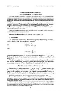
and are feawhere sible points of (P) and (D), respectively. In other words, if a feasible primal-dual pair satisfies (30) and (31), then the pair is optimal. A. Properties of the Separable SDPs (P) and (D) Assume that the parameters of problem (P) satisfy (32) (33) Fig. 1. The primal approach ffis based on iterative purification steps (rank reduction steps) while the dual approach is based on solving an LP in one single step. (a) Primal approach. (b) Dual approach.

solution of its dual problem is explored so as to produce a rank-constrained (e.g., rank-one) solution of the (primal) separable SDP. Interestingly, the rank profile of the output solution is controllable by the user in some sense as it will be later described, and the desired optimal solution can be found by solving an LP in one single step, which is in contrast to the iterative rank reduction steps (i.e., the purification steps) described in Algorithm 1 derived from the primal perspective (see Fig. 1 for a pictorial comparison). Consider the following separable SDP and its dual:

In particular, the SINR constraints of OBP [cf. (12)] have their parameters fulfilling (32) and (33). Due to the assumptions (32) and (33), problems (P) and (D) have some specific properties, the proofs of which are based on feasibility and complementarity of (P) and (D). Proposition 4.1: Suppose that the parameters of (P) satisfy (32) and (33), and that both SDPs (P) and (D) are solvable, and , with solutions respectively. Then , ; (i) (ii) , and , . Proof: See Appendix B. Let us further assume that the parameters satisfy (34) and (35)

(27)

and

where

(28) (29)

and , , are defined in (16). The complementary conditions for the primal and dual SDPs (P) and (D) are (30) (31)

, (asNote that (35) implies that suming problem (P) is feasible). Particularly, the soft-shaping interference constraints of (OBP) comply with assumption (35), and the parameters of the objective function of (OBP) satisfy the assumption (34). Proposition 4.2: Suppose that the parameters of (P) satisfy (32)–(35), and that both SDPs (P) and (D) are solvable, with soand , respeclutions tively. Then, . Proof: See Appendix C. Now, let us investigate some properties of the optimal solution set of dual SDP (D). We define the set shown in (36) at . In the bottom of the page, given , the set defined in (36) reduces the particular case of to (37), shown at the bottom of the page, and it is seen that for . is an optimal solution of (D) Assume that and (P) is solvable and the parameter assumptions (32) and (33) are satisfied, it thus follows from Proposition 4.1 that

(36)

(37)



4261

. Additionally assume that the parameter assumptions (34) and (35) are fulfilled, it then follows from the complementary condition (30) that the opin timal solutions of (P) must be of rank one if the matrices are of rank (it is the case, for instance, are of rank one, i.e., , where , when matrices , are the channel vectors). In addition, the following result gives an explicit characterof set , ization of the elements is given. where Proposition 4.3: Suppose that is , where the paramgiven and , fulfill (32), (34) and (35). Then, eters , , (i) ; where (ii) , , amounts and , ; to contains only one point with (iii) the set , . Proof: See Appendix D. We remark that when , it follows from Proposition 4.3 (iii) that the optimal solution of problem (D) is unique. In particular, the dual of the OBP with only SINR constraints (no soft-shaping constraints) has an unique optimal solution. B. Rank-One Solution of Separable SDP Via Linear Programming Here, we consider the separable SDP (P) with the first con) and propose an efficient algorithm by straints only (i.e., solving a linear program based on observations of the previous there subsection. From Theorem 3.1, we know that for always exists a rank-one solution, which we are about to present a new way to output. Other interesting results on problem (P) involving more types of constraints will be presented in the next section. The problem and its dual are

(38)

and

(39) and are defined in (29) and (16), respectively, where and we assume that the parameters of problem (P1) satisfy conditions (32)–(34). Observe that the SDP relaxation problem of the OBP of Section II with only SINR constraints belongs to the class of problem (P1). Suppose that both (P1) and (D1) are solvable, and and be oplet timal solutions of (P1) and (D1), respectively. It fol, , lows from Proposition 4.1 that and , , and from Proposition 4.2 that . In other of words, we can safely change the general inequalities without loss of generality. problem (P1) into inequalities and Therefore, from now on we will consider each the corresponding in (38) and (39). defined in (37) is equivalent to It is clear that the set (40), shown at the bottom of the page. Given the solution , the corresponding in (40) can be taken as follows: , , for . In an and . alternative way, one may take and (from the complemenIndeed, since tary condition (30)), it follows that and . Now, let us investigate how to retrieve a rank-one solution of , each component of which could be of (P1) from arbitrary rank. We formulate the following LP shown in (41) at the bottom of the page. Note that vectors are fixed parameters and not part of the optimization. This LP possesses the key of properties that it is feasible (since the solution (D1) is feasible to (LP1)) and bounded below (since and , ). Thus, it follows by the duality theorem of LP

(40)

(41)


4262


(for example, see [16, Theorem 1.2.2]) that both (LP1) and its dual (DLP1) are solvable

(42) and be optimal solutions of Let (LP1) and (DLP1), respectively. Then, the complementary conditions of (LP1) and (DLP1) are satisfied

We remark that when solving (P1) with the parameter assumptions (32) and (33), Algorithm 1 (from the primal perspec, i.e., a tive) gives a solution of rank rank-one solution (since , ), while the additional parameter assumption (34) allows us to find a rank-one solution of (P1) by Algorithm 2 (from the dual perspective). As shall be seen in the next subsection, the dual approach can also provide a of (P1) with a more arbitrary rank prosolution , , where is file satisfying a prefixed rank profile. C. Separable SDP’s Solution With a Given Rank Profile

(43)

(44) These two LPs are very useful and we will see that problem (DLP1) provides rank-one optimal solutions to (P1). To proceed, let us denote .. .

..

.. .

.

.. .

and

(45)

Theorem 4.4: Suppose that the parameters of (P1) satisfy (32)–(34). Suppose that both (P1) and (D1) are solvable and let be an optimal solution of (D1). Take with , , and formulate any vectors be an optimal the two LPs (LP1) and (DLP1). Let solution of (DLP1). Then, (i) , ; , ; (ii) ; (iii) defined in (45) is invertible, and , where (iv) represents the optimal value of problem ; and is optimal for (P1). Proof: See Appendix E. It follows from Theorem 4.4 that a rank-one solution of (P1) can be obtained by solving (DLP1), the formulation of which is based on an optimal solution of (D1), and that (DLP1) has always the closed-form solution. In other words, a rank-one solution of SDP (P1) can be found by solving its dual and an LP. Algorithm 2 summarizes the procedure to generate a rank-one solution of (P1). Algorithm 2: Procedure for Rank-One Solution of Separable SDP , , , , , satisfying (32)–(34); with

,

; ;

1:solve the dual SDP (D1), finding ,

2:take unit-norm vectors 3:form the matrix 4:output

as in (45), and compute ,

.

; ;

In this subsection, we show that the above LP approach can also be used to provide an optimal solution to the separable SDP (P1) satisfying a prefixed rank profile, not merely rank-one solution. One motivation of imposing a rank profile lies in the robust design of the multiple transmit beamforming architecture for a MIMO communication with transmission using OSTBC, as described in Section II-A. Besides, another motivation comes from the setting of a cognitive MIMO radio network; in order to transmit over the same frequency band but without interfering, a secondary transmitter has an antenna array and uses multiple beamforming to put nulls over the directions identifying the primary receivers and make the degradation induced on the primary users performance null or tolerable (see [14]). , is an optimal solution Suppose that of (D1). Let , . It follows and , thus for from Proposition 4.1 that . Suppose that a rank profile is given. of The goal now is to find an optimal solution problem (P1) such that , . of (P1), together with Since any optimal solution , fulfills the complementary condition (30), i.e., , , the rank of (i.e., the dimension of the range of ) cannot be more than . Based on the observation, we with for each . In particular, when substitute , , we can output a the rank profile is specified by desired solution of (P1) with Algorithm 2. , , Take any unit norm vectors , such that are orthogonal vectors, for each , and formulate the following LP shown in (46) at the of bottom of the next page. Note that a solution (D1) is feasible for (LP2), and (LP2) is bounded below (since and , ), and it follows again by the LP strong duality theorem that (LP2) and its dual problem (DLP2), shown in (47) at the bottom of the next page, are solvable. Similarly to Theorem 4.4, an optimal solution of (DLP2) yields a rank-constrained solution to (P1). Theorem 4.5: Suppose that the parameters of (P1) satisfy (32)–(34), and that both (P1) and (D1) are solvable. , be given positive integers, and let Let , be an optimal solution of (D1). unit-norm vectors such that Take any are orthogonal, , and formulate the LPs (LP2) and (DLP2). Let be an optimal solution of (DLP2). Then, , ; (i)



(ii) at least one of ; (iii)

4263

is positive, for any , and is an op-

timal solution of (P1). Proof: See Appendix F. It is seen easily that the optimal solution obtained in Theorem and at least one, . Algorithm 4.5 has rank no more than 3 summarizes the procedure to produce an optimal solution of (P1) complying with a prescribed rank profile. Observe that the can be achieved only if specified rank profile ; otherwise, we can only achieve as indicated in Algorithm 3. Algorithm 3: Procedure for Solution of Separable SDP Problem With a Given Rank Profile , , , , satisfying (32)–(34); the rank profile ; with

,

; ;

1:solve the dual SDP (D1), finding ,

2: 3:substitute

with

; ;

, 4:take any vectors are orthonormal, for

, such that ;

5:form the linear program (DLP2), and solve it, finding , ; 6:output

.

,

V. SEPARABLE SDP WITH INDIVIDUAL SHAPING CONSTRAINTS VIA LINEAR PROGRAMMING We consider now a separable SDP problem with additional individual shaping constraints:

(48) , , , , comply with aswhere the parameters , . Its dual problem sumptions (32)–(34) and , is shown in (49) at the bottom of the page, where , are defined in (16). In this section, again resorting to an LP approach, we build an efficient algorithm to find a rank-one optimal solution of (P2), which is in contrast with the iterative , of rank reduction procedure for (P2) with two groups, individual shaping constraints as in [5]. Suppose that both problems (P2) and (D2) are solvable, and , be let optimal solutions of (P2) and (D2), respectively. It follows by the strong duality theorem (e.g., [16, Th. 1.7.1]) that they satisfy . the complementary conditions (18)–(20) with Let us highlight some properties of the primal and dual optimal solutions as next proposition. Proposition 5.1: Suppose that the parameters of (P2) satisfy (32)–(34), and that both (P2) and (D2) are

(46)

(47)

(49)


4264


solvable,

with

solutions

and , respectively. Then,

, ; (i) (ii) , and , ; and , . (iii) Proof: See Appendix G. From the above proposition, we observe that either changing to or changing all all general inequalities to will not lose any generality in problem (P2). Thus, from and the corresponding now on we consider every in (48) and (49). A. Individual Semidefinite Shaping Constraints

Algorithm 4: Procedure for Rank-One Solution of Separable SDP Problem With Individual Semidefinite Shaping Constraints ,

,

(51) We state some important properties of the LPs in the theorem. Theorem 5.2: Suppose that the parameters of (P2) comply with (32), (33), and (17). Suppose that both and (P2) and (D2) are solvable and let be optimal solutions of (P2) and (D2), respectively. Take any unit-norm vectors , , and formulate the LPs (LP1) and (DLP1). Then, is feasible for (i) (LP1) is bounded below, and (LP1) (i.e., both (LP1) and (DLP1) are solvable). be an optimal solution of (DLP1) and suppose Let , fulfill (34). Then, that , (i) , , and , , and where is defined in (45); , and (ii) is an optimal solution of (P2). Proof: See Appendix H. Algorithm 4 summarizes the procedure to produce a rank-one optimal solution of (P2).

, , , , satisfying (32)–(34) and (17);

an optimal solution , ;

of (P2), with ,

1:solve SDPs (P2) and (D2), finding solutions ; and ,

2:take unit-norm vectors ; 3:form the matrix

We consider separable SDP (P2) with individual shaping constraints where each is semidefinite, i.e., all satisfy (17). and Let be optimal solutions of (P2) and (D2), respectively. , , since We can take a unit-norm vector , , and the formulate the LP problem shown in (50) at the bottom of the page, and its dual

,

4:output


;

.

It is interesting to remark that the optimal value of problem (50) is no less than that of problem (41), due to the fact that and the choice of in (50) and (41) is different. Also, it is noted that a rank-one solution of (P1) with individual semidefinite shaping constraints can be output by applying the preprocess procedure introduced in Section III-A (the paragraph containing (22)) and Algorithm 2. We point out that like in Section IV-C, it is possible to conwith the difference sider an arbitrary rank profile that one has to solve (D2) and (P2) in Step 1 of Algorithm 3. B. Individual Indefinite Shaping Constraints In this subsection, we consider the separable SDP (P2) where some of the individual shaping constraints are indefinite. In particular, assume (52) but with indefinite , , , i.e., they could be any Hermitian matrix. We highlight that the SDP relaxation problem nullof the OBP of Section II with SINR constraints, shaping interference constraints and two groups of individual indefinite shaping constraints, belongs to this class of problem. By some specific rank-one matrix decomposition [17], we will show that problem (P2) with individual shaping constraints (52) have a rank-one solution, which can be generated from an optimal solution of (DLP1). Let us quote the useful matrix decomposition theorem in order to proceed. Lemma 5.3 [17]: Suppose that is a complex Her, are mitian positive semidefinite matrix of rank , and given Hermitian matrices. Then, there is a rank-one two

(50)



4265

TABLE I SOLVABLE INSTANCES OF OPTIMAL MULTIUSER DOWNLINK BEAMFORMING PROBLEM (OBP)

decomposition of

, (synthetically denoted as such that

),

Algorithm 5 summarizes the procedure to produce a rank-one optimal solution of (P2): Algorithm 5: Procedure for Rank-One Solution of Separable SDP Problem With Individual Indefinite Shaping Constraints ,

. and be optimal solutions of (P2) and (D2) respecand , tively, and let . It follows by Lemma 5.3 that we can find a rank-one decomfor each such that position

,

Let

,

, , , , satisfying (32)–(34) and (52);

an optimal solution , ;

, . Then, take , , and formulate linear program (LP1) and its dual (DLP1), as displayed in (50) and (51) respectively. We claim problem (P2) has some properties similar to those in Theorem 5.2 with parameters satisfying (32), (33), and (52). Theorem 5.4: Suppose that the parameters of (P2) comply with (32), (33) and (52). Suppose that both and (P2) and (D2) are solvable, and let be optimal solutions of (P2) and (D2) respectively. Perform the rank-one decomposition for each , yielding , where , so that ; take vectors from , , and formulate the LPs (LP1) and (DLP1). Then, (i) (LP1) is bounded below, and is feasible for (LP1) (i.e., (LP1) and (DLP1) are solvable). Let be an optimal solution of (DLP1). Suppose that , , fulfill (34). Then, (i) , , and , , and , where is defined in (45); (ii) , and is an optimal solution of (P2). Proof: See Appendix I.

,

1:solve SDPs (P2) and (D2), finding solutions ; and ,

2:perform the rank-one decompositions outputting , where ; ,

3:take vectors Observe that

with

4:form the matrix 5:output

;


,

;

.

Last, we mention that it is possible to generate a rank-constrained solution of (P2) with a given rank profile using Algorithm 3, but with the difference that in Step 1 of Algorithm 3 one has to solve (D2) and (P2) and additionally implement the specific rank-one decompositions. VI. SUMMARY OF SOLVABLE INSTANCES OF OBP In this section, we summarize all known solvable instances of the general QCQP downlink (unicast) beamforming problem (OBP) (see Table I), as well as an account of the complexity of the algorithms. We remark that when problem (OBP) has soft-shaping constraints (in additional to SINR constraints and individual shaping constraints), only the primal method (cf. Algorithm 1) can be employed (the dual-based Algorithms 2, 4, and 5 cannot be used). When the problem has no soft-shaping constraints, the dual-based method is preferred due to its lower computational complexity as elaborated next. We now compare the computational complexity of the primal and dual methods when solving the beamforming problem (OBP) with only SINR constraints. The primal method consists of solving the separable SDP, which has a worst-case


4266


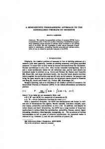
complexity of , where is the desired accuracy of the solution (cf. [16]), and the iterative rank reduction procedure, each step of which contains a eigenvalue flops and decomposition that requires (i.e., solving the system finding the null space of of linear equations ) that requires flops with . The dual method requires solving the same separable SDP and finding the vectors in the respective null spaces and computing the closed-form solution of the LP which involves flops. As to finding ’s, it can be done very efficiently by simply computing the eigenvector corresponding (instead of the null space to the maximum eigenvalue of of the dual solution4) and that can be done efficiently with the power iteration method (see [18, pp. 330–332]), whose . Although the computational complexity is primal method has a higher complexity, it solves a separable SDP (outputting a rank-constrained solution) which has more flexibility on the parameter restrictions, e.g., all do not have to be positive definite, the inequality directions of the global shaping constraints [cf. (4)] can be arbitrary, and parameters in the global shaping constraints can be any Hermitian matrix, and so forth. VII. NUMERICAL EXAMPLES The present section is aimed at illustrating the effectiveness of the proposed downlink algorithms for the optimal beamforming problem. We consider a simulated scenario with a base station feeding signals simultaneously to three single-antenna users, and in problem (OBP). The users are placed i.e., , and relative to the array broadat side of the base station. The channel covariance matrix for users is generated according to (see [3]) (53) , where is the angular spread of local scatterers surrounding user (as seen from the base station) and represents the number of transmit antenna elements equipped for each in the base station. The noise variance is set user. The SINR threshold value for all the three users is set to a common . We make use of the optimization package CVX (see [19]) to solve the SDPs. 1) Simulation Example 1: In this example, we present simulation results when problem (OBP) has multiple null interference constraints beside the SINR constraints, and show how the total transmission power is affected by the number of null interference constraints. In addition to internal users, we consider , ) external users belonging to other six (i.e., coexisting wireless systems, and they are located respectively , , relative to the array broadside of at antenna elements. The channel the base station with is given by (asbetween the base station and external user suming a uniformly spaced array at the base station): (54)

Fig. 2. Minimal transmission power versus the threshold of SINR, with different numbers of null interference constraint.

where , (i.e., the antenna elements are spaced half a wavelength). This corresponds to SINR constraints and problem (OBP) with null interference constraints (or, equivalently, six groups of individual shaping constraints). Fig. 2 illustrates the minimal total transmission power versus the required SINR for the cases of no null interference constraint, two null interference constraints and ), four null interference constraints (with and in addition to and ), and six (with and in null interference constraints (with addition to , ). It can be seen from the figure that higher and higher total transmission power is required to satisfy null interference constraints for more and more external users, as well as the same SINR level to the three internal users. 2) Simulation Example 2: This example shows the results for problem (OBP) where the base station is antenna elements and nine equipped with null interference constraints for nine external users at , together with the three SINR constraints, are involved. In order to illustrate the effect of the additional null interference constraints, we evaluate the power radiation pattern of the base , according to station, for (55) where is a triple of optimal beamvectors, and is defined in (54). Fig. 3 displays the radiation pattern of the (the minimal base station with the SINR threshold value required transmission power is 15.95 dBm). 3) Simulation Example 3: In this example, we consider the robust null-shaping interference constraint [cf. (8)] in the direc), and this can be retion of an external user (say, located at alized by adding two null interference constraints: (56) and

4It is not necessary to characterize the whole null space, whose cost would be

higher. Authorized licensed use limited to: Chinese University of Hong Kong. Downloaded on July 13,2010 at 10:49:33 UTC from IEEE Xplore. Restrictions apply.

(57)


4267

Fig. 3. Radiation pattern of the base station, for the problem with three SINR . The constraints and nine null-shaping interference constraints and required transmit power is 15.95 dBm.

K = 12

where

(58) and is the same as the one in and (54). To better control the robust region of the null-shaping interference around external user , we introduce two more null interference constraints for the external user

Fig. 4. Radiation pattern of the base station, for the problem with three SINR constraints, one null interference constraint, two robust null interference con. The required transmit power is 16.94 dBm. straint, and

K=8

problem. The presented algorithms mainly consist of solving the SDP relaxation of the problem, formulating an LP by using the properties of optimal solution of the dual SDP, and solving the LP (with closed-form solution) to find a rank-one optimal solution of the separable SDP. The proof is based on the LP strong duality. The resulting algorithms can output a rank-one solution, as well as a rank-constrained solution with a prefixed rank profile. Based on these, we have identified the subclasses of the optimal beamforming problem that are “hidden” convex, in the sense that the corresponding SDP relaxation has always a rank-one optimal solution. APPENDIX

(59) for . In other words, there are four constraints [i.e., (56), (57), and (59)] describing a robust nullshaping interference constraint around user . Assume that the transmit antennas, and three external base station has are considusers located, respectively, at ered beside the three internal users. For external user , we impose only one null interference constraint on it, and , we imwhile for external users pose one robust null interference constraint on each of them. Therefore, the resulting optimal beamforming problem has three SINR constraints and nine null interference constraints. Fig. 4 depicts the radiation pattern of the base station (the required minimal transmission power is 16.94 dBm). As expected, the and is sufficiently power radiated over lower so that it is almost negligible.

A. Proof of Theorem 3.1 Proof: The proof is just slightly different from that of [5, Lemma 3.1] (see [5, pp. 675–676]) when checking the primal feasibility and complementarity (optimality) in each iteration of the purification process (rank reduction procedure). , Precisely, we need to additionally verify , and , , , , and where . Indeed, if , then , ; if , and . Since all columns of then it is evident that are in , hence , . B. Proof of Proposition 4.1 that

, . In fact, suppose Proof: (i) First of all, we show , then one has the contradiction

VIII. CONCLUSION In this paper, we have considered the optimal beamforming problem minimizing the transmission power subject to SINR constraints, global and individual shaping interference constraints (e.g., to protect other users from coexisting systems). Although the problem belongs to the class of separable homogeneous QCQP which is typically hard to solve in general, we have proposed efficient algorithms for the beamforming

due to the parameter conditions (32) and (33). , and , . Suppose (ii) Now, we show , for some , say ; then , from the complementary condition (30). However, this is not , . possible since we have shown the fact that


4268


C. Proof of Proposition 4.2 , , and , hence, for those with , for those with , and for . In order to show , , we shall first prove the fact that for (or more precisely, for ). Assume, without loss of generality, that , , , , , , for some . Then, , together with , , is feasible for problem (D), and has the objective function . Thus value cannot be optimal, which is a contradiction. Therefore, we have , . Let us check the feasibility of . In, one has deed, for , where the first relation is due to , and the second is due to the assumption that , , for , . For , one also has , due to for , for , (32), (34), and (35). Now we wish to prove . Suppose that , say , then one of , which is a contradiction to that we have shown in Proposition 4.1. , It follows from (31) that . Proof: Since

,

D. Proof of Proposition 4.3 , and the assumptions (32), (35), (34) are valid, hence, it follows from (36) that each has at least one positive eigenvalue. (i) Suppose is defined by the point as in set , and let Proof: Since

Clearly,

,

. Then, we have

(60)

, , has at least one positive Recall that each , . eigenvalue, thus From (60), it follows that leads to , for (for either the case that is positive semidefinite and nonzero, or the case has both positive and negative eigenvalues). Since that (from the definition of ), then , . (ii) From (60), we see that implies and , , and that implies , , and implies , that . (iii) Suppose that there exists such that . Then it follows from (i) that , . , and suppose that Let without loss of generality (otherwise let ). Also suppose that , . It follows that

, which would . imply But this is not possible since . It follows from the proof of (ii) that the set is a singleton and contains the point: See the equation at the bottom of the page. E. Proof of Theorem 4.4 Proof: (i) Since both (LP1) and (DLP1) are solvable, we suppose that is an optimal solution of (LP1). Thus, and satisfy the complementary conditions (43) and (44). of To proceed, we claim that any feasible point , . To see this, (LP1) must be positive, i.e., , then by the parameter assumptions, one has assume that the contradiction

Consequently, every must be positive. Now, from (44), this , . implies that (ii) Note that each has at least one positive eigenvalue , , from (41). Indeed, if some is negand ative semidefinite, then problem (P1) is infeasible, which contradicts the assumption that (P1) is solvable. Also



and

4269

, , since (from Proposition 4.2). It follows that

the second paragraph of the proof of Theorem 4.4). Thus . It follows from (62) that

It , since and ( ) from the parameter assumptions (32) and (33). (iii) We claim that satisfying (i) and (ii) must be unique, i.e., the solution for the system of and is is another solution for the system, unique. Suppose that . Without loss of generality, and let and ; thus we have we assume that , , which implies that and , . Then one gets the contradiction . Suppose that the square matrix is singular, then there is a such that , and since , we have that nonzero . This implies that the vector for sufficiently small is a solution for the system of and , which is not possible since the system has only one solution. Therefore, is invertible, which yields . If , then (DLP1) has no optimal solution, which is contradictory to the solvability of (DLP1). (iv) It suffices to prove the inequality chain . It is clear that and , due to strong of (D1) is duality. Notice that the optimal solution also feasible for (LP1), and that (D1) and (LP1) have the same . objective function, then we can assert that is feasible Likewise, observing that . Therefore, we for (P1), we conclude that arrive at . Further, is optimal for (LP1) and it is easily verified that is optimal for (P1). F. Proof of Theorem 4.5 Proof: This proof is similar to that of Theorem 4.4. (i) Assume that is an optimal solution of (LP2). , together with the solution , complies Thus, with the complementary conditions of (LP2) and (DLP2)

(61) , and

(62) It is easily seen from (46) that any feasible point of (LP2) is positive, i.e., , (due to a similar argument to

(ii) Suppose that follows from (i)

, that

,

, are zero.

, which is not true since the left-hand side (LHS) is nonpositive and the right-hand side (RHS) is positive. We thus conclude that at least one element is positive, . of (iii) The proof is similar to the proof of (iii) of Theorem 4.4, and thus omitted. G. Proof of Proposition 5.1 Proof: Applying Proposition 4.1 (with ) to (P2) and (D2), one concludes that (i) and (ii) hold. It follows and , from (18)–(20) that . Indeed, from (18) and (20), we have

which means that cannot be zero for any (otherwise, say , then which is not possible).

and

H. Proof of Theorem 5.2 Proof: (i) It is easily seen that (LP1) is bounded below, due and the assumptions . Now, we to the constraints of (D2) is feasible wish to show that the solution for (LP1). , , hence Since . Combining the complementary condition in (20) with the fact that yields (63) Therefore, , and is feasible for (LP1). accordingly Since (LP1) is bounded below and feasible, hence it follows by the strong duality theorem for LP that both (LP1) and (DLP1) are solvable. (ii) The proof is completely similar to those of (i), (ii), and (iii) of Theorem 4.4, and we skip it here. fulfills the (iii) It is easily seen that , individual shaping constraints, that is, , . This, together with (ii), gives that for feasible to (P2), hence, we have . Since the optimal soluof (D2) is feasible for (LP1), hence, tion . Thus, we arrive at the inequality chain


4270


, and it is is optimal to (P2).

easily seen that I. Proof of Theorem 5.4 Proof: (i) We show that Observe that the vectors , have the property

is feasible to (LP1). ,

It thus follows from the complementary condition (20) that and Hence from (63) that

Therefore, is feasible to (LP1). It is evident that (LP1) is bounded below. (ii) The proof is the same as that of (ii) of Theorem 5.2. (iii) From the proof of (iii) of Theorem 5.2, we know that satisfies the individual semidefinite shaping constraints, i.e., Further, the solution also satisfies the indefinite shaping constraints, i.e., As a matter of fact,

This combining with (ii) leads to that is feasible for (P2). By the same argument as the last paragraph of the proof of Theorem 5.2, we conclude that , and that and are optimal for (P2) and (LP1), respectively.

[3] M. Bengtsson and B. Ottersten, “Optimal transmit beamforming using semidefinite optimization,” in Proc. 37th Ann. Allerton Conf. Commun., Contr., Comput., Sep. 1999, pp. 987–996. [4] D. Hammarwall, M. Bengtsson, and B. Ottersten, “On downlink beamforming with indefinite shaping constraints,” IEEE Trans. Signal Process., vol. 54, pp. 3566–3580, Sep. 2006. [5] Y. Huang and D. P. Palomar, “Rank-constrained separable semidefinite programming with applications to optimal beamforming,” IEEE Trans. Signal Process., vol. 58, pp. 664–678, Feb. 2010. [6] F. Rashid-Farrokhi, K. R. Liu, and L. Tassiulas, “Transmit beamforming and power control for cellular wireless systems,” IEEE J. Sel. Areas Commun., vol. 16, pp. 1437–1450, Oct. 1998. [7] M. Schubert and H. Boche, “Solution of the multiuser downlink beamforming problem with individual SINR constraints,” IEEE Trans. Veh. Technol., vol. 53, no. 1, pp. 18–28, 2004. [8] Z.-Q Luo and T.-H Chang, “SDP relaxation of homogeneous quadratic optimization: Approximation bounds and applications,” in Convex Optimization in Signal Processing and Communications, D. P. Palomar and Y. Eldar, Eds. Cambridge, U.K.: Cambridge Univ. Press, 2010, ch. 4. [9] N. Sidiropoulos, T. Davidson, and Z. Q. Luo, “Transmit beamforming for physical-layer multicasting,” IEEE Trans. Signal Process., vol. 54, pp. 2239–2251, Jun. 2006. [10] E. Karipidis, N. Sidiropoulos, and Z.-Q. Luo, “Quality of service and max-min fair transmit beamforming to multiple cochannel multicast groups,” IEEE Trans. Signal Process., vol. 56, pp. 1268–1279, Mar. 2008. [11] T.-H. Chang, Z.-Q. Luo, and C.-Y. Chi, “Approximation bounds for semidefinite relaxation of max-min-fair multicast transmit beamforming problem,” IEEE Trans. Signal Process., vol. 56, pp. 3932–3943, Aug. 2008. [12] Z.-Q. Luo, W.-K. Ma, A. M.-C. So, Y. Ye, and S. Zhang, “Semidefinite relaxation of quadratic optimization problems,” IEEE Signal Process. Mag., vol. 27, no. 3, pp. 20–34, 2010. [13] A. Pascual-Iserte, D. P. Palomar, A. Pérez-Neira, and M. Lagunas, “A robust maximin approach for MIMO communications with imperfect channel state information based on convex optimization,” IEEE Trans. Signal Process., vol. 54, pp. 346–360, Jan. 2006. [14] G. Scutari, D. P. Palomar, and S. Barbarossa, “Cognitive MIMO radio: Competitive optimality design based on subspace projections,” IEEE Signal Process. Mag., vol. 25, no. 6, pp. 46–59, Nov. 2008. [15] M. H. Er and B. C. Ng, “A new approach to robust beamforming in the presence of steering vector errors,” IEEE Trans. Signal Process., vol. 42, pp. 1826–1829, Jul. 1994. [16] A. Nemirovski, Lectures on Modern Convex Optimization, Class Notes Georgia Inst. Technol., 2005 [Online]. Available: http://www2.isye. gatech.edu/~nemirovs/Lect_ModConvOpt.pdf [17] Y. Huang and S. Zhang, “Complex matrix decomposition and quadratic programming,” Math. Operat. Res., vol. 32, no. 3, pp. 758–768, 2007. [18] G. H. Golub and C. F. Van Loan, Matrix Computations. Baltimore, MD: The Johns Hopkins Univ. Press, 1996. [19] M. Grant and S. Boyd, CVX: Matlab Software for Disciplined Convex Programming Dec. 2008 [Online]. Available: http://stanford.edu/~boyd/cvx

ACKNOWLEDGMENT The authors would like to thank Associate Editor Dr. X. Mestre and the three anonymous reviewers for the helpful comments toward the improvement of this paper. The authors also would like to thank Prof. W.-K. (Ken) Ma for discussions and, in particular, pointing out (iii) of Theorem 4.4 to us. REFERENCES [1] A. B. Gershman, N. D. Sidiropoulos, S. Shahbazpanahi, M. Bengtsson, and B. Ottersten, “Convex optimization-based beamforming: From receive to transmit and network designs,” IEEE Signal Process. Mag., vol. 27, no. 3, pp. 62–75, 2010. [2] M. Bengtsson and B. Ottersten, “Optimal and suboptimal transmit beamforming,” in Handbook of Antennas in Wireless Communications, L. C. Godara, Ed. Boca Raton, FL: CRC, 2001, ch. 18.

Yongwei Huang (M’09) received the B.Sc. degree in computational mathematics in 1998 and the M.Sc. degree in operations research in 2000, both from Chongqing University. In 2005, he received the Ph.D. degree in operations research from the Chinese University of Hong Kong. He was a Postdoctoral Fellow with the Department of Systems Engineering and Engineering Management, the Chinese University of Hong Kong, and a Visiting Researcher of the Department of Biomedical, Electronic, and Telecommunication Engineering, University of Napoli “Federico II,” Italy. Currently, he is a Research Associate with the Department of Electronic and Computer Engineering, the Hong Kong University of Science and Technology. His research interests are related to optimization theory and algorithms, including conic optimization, robust optimization, combinatorial optimization, and stochastic optimization, and their applications in signal processing for radar and wireless communications.



Daniel P. Palomar (S’99-M’03-SM’08) received the electrical engineering and Ph.D. degrees (both with honors) from the Technical University of Catalonia (UPC), Barcelona, Spain, in 1998 and 2003, respectively. Since 2006, he has been an Assistant Professor with the Department of Electronic and Computer Engineering, Hong Kong University of Science and Technology (HKUST), Hong Kong. He has held several research appointments, namely, at King’s College London (KCL), London, U.K.; Technical University of Catalonia (UPC), Barcelona; Stanford University, Stanford, CA; Telecommunications Technological Center of Catalonia (CTTC), Barcelona; Royal Institute of Technology (KTH), Stockholm, Sweden; University of Rome “La Sapienza,” Rome, Italy; and Princeton University, Princeton, NJ. His current research interests include applications of convex optimization theory, game theory, and variational inequality theory to signal processing and communications.

4271

Dr. Palomar is an Associate Editor of the IEEE TRANSACTIONS ON SIGNAL PROCESSING, a Guest Editor of the IEEE Signal Processing Magazine 2010 Special Issue on “Convex Optimization for Signal Processing,” was a Guest Editor of the IEEE JOURNAL ON SELECTED AREAS IN COMMUNICATIONS 2008 Special Issue on “Game Theory in Communication Systems,” as well as the Lead Guest Editor of the IEEE JOURNAL ON SELECTED AREAS IN COMMUNICATIONS 2007 Special Issue on “Optimization of MIMO Transceivers for Realistic Communication Networks.” He serves on the IEEE Signal Processing Society Technical Committee on Signal Processing for Communications (SPCOM). He is a recipient of a 2004/2006 Fulbright Research Fellowship; the 2004 Young Author Best Paper Award by the IEEE Signal Processing Society; the 2002/2003 best Ph.D. prize in Information Technologies and Communications by the Technical University of Catalonia (UPC); the 2002/2003 Rosina Ribalta first prize for the Best Doctoral Thesis in Information Technologies and Communications by the Epson Foundation; and the 2004 prize for the best Doctoral Thesis in Advanced Mobile Communications by the Vodafone Foundation and COIT.


A Dual Perspective on Separable Semidefinite Programming With ...

A Dual Perspective on Separable Semidefinite Programming With ...

Suggest Documents

Semidefinite Programming

Semidefinite Programming

Semidefinite Programming and Constraint Programming

Robust Semidefinite Programming - ISyE

Unsupervised Image Partitioning with Semidefinite Programming Jens ...

Learning the Kernel Matrix with Semidefinite Programming

ROBUST FILTERING VIA SEMIDEFINITE PROGRAMMING WITH ...

Formulating Face Verification With Semidefinite Programming

On Doubly Positive Semidefinite Programming ... - Optimization Online

On robust semidefinite programming - UCSD Mathematics

A Matlab software for semidefinite programming with bound

A Dynamical Systems Analysis of Semidefinite Programming with ...

A Linear Programming Approach to Semidefinite ...

Approximation Clustering: a Mine of Semidefinite Programming ...

A semidefinite programming approach to the

A Matlab software for semidefinite programming with bound ... - arXiv

A SEMIDEFINITE PROGRAMMING APPROACH ... - Semantic Scholar

A Sequential Convex Semidefinite Programming ... - Optimization Online

SDU: A Semidefinite Programming-Based ... - Semantic Scholar

A Semidefinite Programming approach for solving Multiobjective ...

A note on the Lovasz-Schrijver Semidefinite Programming Relaxation ...

InfeasibleâStart Semidefinite Programming ...

A Signaling Perspective on EmploymentBased Reentry Programming

a perspective on combining different programming ...

A Dual Perspective on Separable Semidefinite Programming With ...