FrankâWolfe method nor the state-of-the-art methods for traffic assignment. We outline ... Optimization, Frank-Wolfe Algorithm, Method of Successive Averages.
A Dual Scheme for Traffic Assignment Problems Torbj¨orn Larsson, Zhuangwei Liu,∗ and Michael Patriksson Department of Mathematics, Link¨oping University, S-581 83 Link¨oping, Sweden Revised August 12, 2014
Abstract A solution method based on Lagrangean dualization and subgradient optimization for the symmetric traffic equilibrium assignment problem is presented. Its interesting feature is that it includes a simple and computationally cheap procedure for calculating a sequence of feasible flow assignments which tend to equilibrium ones. The Lagrangean subproblem essentially consists of shortest route searches, and it is shown that one may compute an equilibrium flow by taking the simple average of all the shortest route flows obtained during the subgradient optimization scheme, provided that its step lengths are chosen according to a modified harmonic series. The new method is compared to the Frank–Wolfe algorithm and the method of successive averages on a medium-scale problem; its computational performance is at least comparable to that of the two other methods. The main motive for considering this computational methodology is that it may easily be extended and applied to more complex traffic problems; this feature is not shared by neither the Frank–Wolfe method nor the state-of-the-art methods for traffic assignment. We outline its extensions to several well-known network models, and illustrate the methodology numerically on one of these, an equilibrium model with link counts; the results obtained are encouraging. Keywords: Traffic Assignment, Traffic Equilibrium, Lagrangean Duality, Subgradient Optimization, Frank-Wolfe Algorithm, Method of Successive Averages.
1
Introduction
The traffic assignment problem is solved to estimate the route flows in each of the origin–destination relations of a road network, and the resulting travel times. There is a large variety of traffic assignment models, but in the following we will mainly consider the basic model with fixed travel demands subject to the user optimum, or equilibrium, condition. The equilibrium condition was enunciated by Wardrop (1952) and states that the travel times on routes that are actually used in an equilibrium situation are equal, that is, they are all shortest at the equilibrium traffic flow. Consider a transportation network G=(N , A). Each directed arc a ∈ A is associated with a positive, continuous function ta : ℜ+ 7→ ℜ++ , measuring the time (or, cost) of traversing the arc as a function of the flow fa on the arc. As a result of congestion, it is natural to assume that these functions are strictly increasing, and tend to infinity with the flow. For certain origin–destination (OD) pairs, (p, q) ∈ C ⊂ N × N , there is a demand dpq of flow, which is here assumed to be fixed. We define the set of simple (loop-free) routes from origin p to destination q by Rpq and denote the flow on route r from p to q by hpqr . We will also use the notations f and h for the vectors of arc and route flows, respectively, and H for the set of route flow solutions that are consistent with the demands. The set of routes that are shortest within an OD pair (p, q) ∈ C in an equilibrium situation is denoted R∗pq . Mathematically, the fixed demand equilibrium Traffic Assignment Problem can then be stated as (see e.g. Dafermos and Sparrow, 1969) ∗ Present address: Department of Mathematics, National University of Singapore, 10 Kent Ridge Crescent, 0511, Singapore
1
[TAP]
min
T (f ) =
XZ
a∈A
s.t.
fa
ta (s)ds
0
X
∀(p, q) ∈ C
hpqr = dpq
(1)
r∈Rpq
X
X
hpqr ≥ 0
δpqra hpqr = fa
∀r ∈ Rpq
∀(p, q) ∈ C
∀a ∈ A
(2) (3)
(p,q)∈C r∈Rpq
fa ≥ 0
∀a ∈ A,
(4)
where (δpqra ) is an arc-route incidence matrix for G, with � 1, if route r ∈ Rpq contains arc a, δpqra = 0, otherwise. As a result of the assumptions made above, the problem [TAP] is a convex optimization problem. It is highly structured and usually very large, and it has therefore inspired a large amount of research devoted to the task of devising specialized methods for solving it efficiently. The standard method utilizes the well known Frank–Wolfe algorithm (Frank and Wolfe, 1956); when adapted to [TAP], the linearized subproblem is a set of shortest route problems. The application of the algorithm to the traffic assignment problem was suggested by Bruynooghe et al. (1969), and LeBlanc et al. (1975) were the first to implement it to solve a realistic problem. The performance of the Frank–Wolfe method is often far from satisfactory, and a lot of research effort has been put into finding improvements of it. LeBlanc et al. (1985) modified the search directions by incorporating the PARTAN technique. Modifications have also been suggested with respect to the step lengths taken in the algorithm, see, for example, Weintraub et al. (1985). Hearn et al. (1987) presented a restricted simplicial decomposition algorithm, in which the line search is replaced by a multi-dimensional search over a set of shortest route patterns. The simplicial decomposition method was extended in Larsson and Patriksson (1992), which also contains a survey of Frank–Wolfe type methods. There have also been some suggestions for solution methods for [TAP] based on duality. However, these methods are either inherently dual, in the sense that primal feasibility is obtained in a limiting case only, or they demand the repeated solution of a non-trivial auxiliary optimization problem in order to retain primal feasibility throughout the solution process. The Lagrangean dual method for traffic assignment problems to be presented in this paper utilizes the same dualization as that used in earlier studies. The dual problem is solved by an iterative subgradient optimization procedure, and embedded in this scheme is an averaging technique which is used to calculate primal feasible solutions; an optimal primal solution is obtained in the limit if the step lengths in the subgradient procedure are chosen according to a modified harmonic series. The resulting solution method is very simple, both from a conceptual and implementational point of view, and extends the Lagrangean dual method for linear programs developed in Larsson and Liu (1997) to the convex program [TAP]. Its merits as compared to earlier dual methods are that it, despite its dual character, produces a feasible flow in each iteration, and, further, that this is done without the solution of any additional optimization problem. It is as simple to implement as the Frank–Wolfe method, but as compared to that method, and its relatives, it can easily be modified to solve more complex traffic assignment type models for which the Frank–Wolfe method is computationally unfeasible. The outline of the paper is as follows. First, in Section 2, we discuss the basic properties of the problem [TAP] and its Lagrangean dual. In particular, we conclude that the problem possesses an inherent noncoordinability in the sense that optimal route flows can, in general, not be obtained from the Lagrangean dual subproblem, even if the exact dual optimum is known. In Section 3, we derive a convergent primal algorithm for the convex program [TAP]. Section 4 reports computational results for the new method applied to a medium-scale test problem and these are also compared to results for the Frank–Wolfe algorithm and the closely related method of Powell and Sheffi (1982). Section 5 gives modifications and extensions of the new method to some related assignment problems. Finally, in Section 6, some conclusions are drawn and topics for further research are discussed.
2
2
Characteristics of the Problem and Its Dual Program
In this section, we establish some properties of the problem [TAP], its Lagrangean dual program, and some of their relations. We also briefly review two known dual solution methods for [TAP]. From the assumptions on the arc performance functions, it directly follows that the objective of [TAP] is strictly convex with respect to arc flows. However, if the arc flow variables are temporarily eliminated from the problem, the objective of the resulting equivalent problem in route flow variables is, in general, only convex, since an arc flow pattern may correspond to several route flow patterns. The following proposition is then immediate. Proposition 1 The problem [TAP] is convex. There is a unique optimal arc flow solution, f ∗ . The set of optimal route flow solutions, H ∗ , is a polytope, and in general it is not a singleton. The set H ∗ is a polytope since it is described by a linear system and is bounded. An interesting property of the convex program [TAP] is that the definitional constraints (3) induce a projection onto a subspace of the feasible set of route flows, defined by (1), (2), (4), where the objective is strictly convex. This property has some interesting consequences when the Lagrangean dual program of [TAP] is studied. Dual formulations and algorithms for traffic assignment type problems have been studied by Hall and Peterson (1976), Rockafellar (1984, Section 11G), Fukushima (1984a, 1984b), Carey (1985), Goffin (1987), and Hearn and Lawphongpanich (1990), among others. (See also Patriksson (1994) for a review and analysis of dual formulations and algorithms.) Letting u = (ua )a∈A denote the Lagrangean multipliers associated with the arc flow defining constraints (3), the dual objective obtained is u 7→ θ(u) := θSR (u) + θSC (u), where [SR]
X
θSR (u) =
X X ( ua δpqra )hpqr
min
r∈Rpq a∈A
(p,q)∈C
X
s.t.
∀ (p, q) ∈ C
hpqr = dpq
r∈Rpq
hpqr ≥ 0
∀r ∈ Rpq , ∀ (p, q) ∈ C,
and [SC]
θSC (u) =
X
min
a∈A
fa ≥0
(Z
fa
ta (s)ds − ua fa
0
)
.
The subproblems [SR] and [SC] decompose into |C| shortest (simple) route problems, and |A| strictly convex single-variable minimization problems, respectively. We introduce the solution sets H(u) =
{ h | h solves the problem [SR] at u },
f (u) =
{ f | f solves the problem [SC] at u },
and let Rpq (u), (p, q) ∈ C, be the simple routes solving [SR] at u. The set H(u) is a polytope, but not a singleton for all u (in particular not at an optimal solution). Some properties of the Lagrangean dual objective θ are summarized in the following proposition. Proposition 2 The dual objective θ is a sum of a concave piecewise linear function, and a strictly concave, differentiable function. It is thus everywhere finite, continuous, concave, and sub-differentiable. Its subdifferential is a bounded polyhedron, given by X X f = f (u), h ∈ H(u) . δpqra hpqr − fa (5) ∂θ(u) = conv (p,q)∈C r∈Rpq (u) a∈A
∗
|A|
Furthermore, θ(u) ≤ T (f ) for all u ∈ R
.
3
Now, let t(0) > 0 be the vector of travel times at zero flows (free-flow travel times). Utilizing that each ta is strictly increasing, and unbounded when the flow tends to infinity, it is easily shown that the subproblem [SC] is solved by � −1 ta (ua ), if ua ≥ ta (0), fa (ua ) = a ∈ A, 0, otherwise, where t−1 a is the continuous inverse mapping (see e.g. Rudin, 1976, p. 90) of ta , a ∈ A. One may note that t−1 a is explicit for most performance functions used, and that ta is not required to be differentiable. Consider an arbitrary dual solution u ¯, and define u ˆ = max{¯ u, t(0)}, where the maximum is taken component-wise. Then, f (ˆ u) = f (¯ u), so that θSC (ˆ u) = θSC (¯ u). Further, θSR (ˆ u) ≥ θSR (¯ u) since u ˆ≥u ¯, and it follows that θ(ˆ u) ≥ θ(¯ u). Since the dual objective is to be maximized over R|A| , one can therefore, without loss of generality, impose the restrictions u ≥ t(0) (see also Fukushima, 1984b). The Lagrangean dual problem may now be stated as [DTAP]
max s.t.
θ(u) u ≥ t(0).
Proposition 3 The Lagrangean dual program [DTAP] is a convex optimization problem with a unique optimal solution, u∗ . Proof: The problem [DTAP] is convex since the concave objective function is to be maximized over a convex feasible set. There is a unique dual optimum since f ∗ is unique and fa = t−1 a is strictly increasing for ua ≥ ta (0), a ∈ A. 2 The dual problem has an interesting interpretation; in contrast to the primal problem [TAP], in which the equilibrium arc flows are sought for, [DTAP] is the problem of determining the equilibrium travel times, u∗ (cf. Fukushima, 1984b). The following proposition relates the primal and dual solutions. Proposition 4 Strong duality holds, that is, θ(u∗ ) = T (f ∗ ). Furthermore, f ∗ = f (u∗ ), X X H ∗ = h ∈ H(u∗ ) δpqra hpqr = fa∗ ⊆ H(u∗ ), ∗ (p,q)∈C r∈Rpq (u )
and R∗pq = Rpq (u∗ ).
Proof: The strong duality follows from the convexity of [TAP] and the fact that a constraint qualification holds (see e.g. Bazaraa and Shetty, 1979, Theorem 6.2.4). Further, the set of optimal solutions of [TAP] may be characterized as the Lagrangean subproblem solutions for u = u∗ which also satisfy the dualized constraints (see e.g. Bazaraa and Shetty, 1979, Theorem 6.5.2). The uniqueness of f (u∗ ) gives f ∗ = f (u∗ ) and the expression for H ∗ follows. The set R∗pq is obtained from a linear approximation of [TAP] at f = f ∗ . Since t(f ∗ ) = u∗ , this linearized problem is equivalent to [SR] defined at u = u∗ . It follows that R∗pq = Rpq (u∗ ). 2 To conclude, the proposition states that the optimal arc flow solution f ∗ is obtained from the subproblem [SC] given u∗ . Further, the set of routes solving [SR], given u∗ , coincide with those that are shortest at equilibrium. However, an optimal route flow pattern h∗ ∈ H ∗ is, in general, not directly available from the subproblem [SR] even though the optimal dual solution is at hand. This is so because H(u∗ ) is usually not a singleton, or, equivalently, because θSR (u) is non-differentiable at u∗ . (In the case where f ∗ is known, an algorithm for calculating an h∗ ∈ H ∗ is given in Drissi-Ka¨ıtouni, 1990.) Fukushima (1984a and 1984b) and Hearn and Lawphongpanich (1990) develop iterative algorithms for [TAP] based on the same dualization as the one made above. The main differences between these
4
algorithms and the proposed one are the techniques employed for solving [DTAP] and obtaining feasible solutions. Below, we discuss in short the methods of Fukushima and Hearn and Lawphongpanich. Fukushima (1984a) considers the traffic assignment problem with elastic demands. A subgradient optimization method (see e.g. Polyak, 1969, and Held et al., 1974) is used for solving the dual problem, and upper bounds on the optimal value are provided by the shortest route assignments obtained when evaluating the dual function. (These upper bounds will, however, in general not converge to the optimal value, since it is highly unlikely that such an assignment is optimal.) In Fukushima (1984b), the subgradient procedure is replaced by a combined proximal point and cutting plane algorithm. The main computational effort of both methods lies in the solution of shortest route problems. A disadvantage of Fukushima’s approaches is that they are essentially dual, because of the non-convergence of the upper bounds (primal optimality is obtained when f (u) becomes feasible, which occurs in the limit only). Hearn and Lawphongpanich (1990) consider the capacitated traffic assignment problem, that is, the traffic assignment problem with explicit upper bounds on the arc flows. For solving the dual problem, they utilize a cutting plane (dual column generation) approach. When applied to [TAP], their method proceeds as follows. For each dual iterate, uk , the evaluation of the dual objective provides a cut, so that the dual problem may be approximated by the linear master problem [DM]
max
w
u,w
w≤
s.t.
XZ
fak
ta (s)ds +
0
a∈A
ua ≥ 0
X
a∈A
∀a ∈ A
ua
X
X
(p,q)∈C r∈Rpq
δpqra hkpqr − fak
∀k ∈ K
where f k = f (uk ), hk ∈ H(uk ), and K is the index set of the subproblem solutions generated so far. Its linear programming dual problem is ! X X Z fak [PM] min ta (s)ds νk ν
s.t.
k∈K
X
k∈K
a∈A
X
0
X
(p,q)∈C r∈Rpq
δpqra hkpqr νk ≤ X
X
fak νk
∀a∈A
k∈K
νk = 1
k∈K
νk ≥ 0
∀ k ∈ K.
This is in fact the master problem in the nonlinear Dantzig–Wolfe algorithm (see e.g. Lasdon, 1970) for [TAP]. (Here, it is utilized that the equality constraints (3) can equivalently be written as inequalities.) A primal optimal solution of [PM] provides a feasible solution to [TAP], and hence an upper bound on its optimal value, while the corresponding dual optimal solution defines a search direction. An approximate line search is then made in the dual space to obtain a new dual iterate. An advantage of this approach is that primal feasibility is retained in all iterations; a disadvantage is that the linear master problem becomes computationally expensive when the number of accumulated columns in [PM] grows, even though a column dropping strategy may be utilized. The dual method for [TAP] to be presented constructs a sequence of feasible route and arc flow solutions, converging to optimal ones, without the need to solve any additional auxiliary optimization problems. An inherent property of the dual objective is its non-differentiability, which is a consequence of the fact that the objective of [TAP] is identically zero, that is, linear, in the route flow variables (and hence not strictly convex in the joint arc and route flow space). In the field of linear programming, the nondifferentiability of Lagrangean dual objectives is indeed well known and studied, and many methods for dealing with it have been developed. The methods to be described in the next section constitute generalizations of those for linear programming in Larsson and Liu (1997), which, in turn, were inspired by results by Shor (1985, Section 4.4).
5
3
A Method for the Traffic Assignment Problem
In this section, we present a new algorithm for solving [TAP]. The main idea of the algorithm is to apply a dual subgradient optimization procedure, in which we embed a scheme for calculating a sequence of primal feasible solutions, which can be shown to tend to an optimal one. The feasible flows are calculated from the shortest route solutions of the linear subproblem [SR]; that feasible solutions are very easily constructed is explained by the fact that the Lagrangean relaxed constraints of [TAP] are definitional; this application is thus particularly well suited for such a dual scheme.
3.1
Theory
We first state a straightforward subgradient optimization scheme, and prove its convergence, as applied to [DTAP]. According to Proposition 2, one can easily obtain a subgradient ξ k of the dual function θ at uk as X X ξak = δpqra hkpqr − fak , a ∈ A, (p,q)∈C r∈Rpq (uk )
where hk solves [SR] for u = uk , and fak = ta−1 (uka ), a ∈ A. The dual solution is updated according to the formula � uk+1 = max uk + γk ξ k , t(0) , k = 1, 2, . . . , (6)
where the maximum is taken component-wise, and u1 = t(0). We will need the following convergence result. Theorem 1 Let the step lengths in the subgradient optimization procedure (6) applied to [DTAP] be chosen according to the divergent series conditions γk > 0,
lim γk = 0,
k→∞
and
∞ X
γk = ∞.
(7)
k=1
Then, the sequence {uk } converges to u∗ . Proof: The result follows from classical arguments used in the analysis of subgradient optimization methods (e.g., Ermol’ev, 1966; Shor, 1985; Larsson et al., 1996), once we have established that the sequence {ξ k } is bounded. P Let γ¯ := supk γk < ∞ (since {γk } → 0) and D := (p,q)∈C dpq , and let U = {u | t(0) ≤ u ≤ t(De) + γ¯ De } ,
where e is a column vector of ones. Assume that uk ∈ U , for some k, and consider some a ∈ A. We then have either of the following two cases. In the first case, ta (0) ≤ uka ≤ ta (D) holds. Then, X X ξak = δpqra hkpqr − fak ≤ D, (p,q)∈C r∈Rpq
so that uk+1 ≤ uka + γ¯D ≤ ta (D) + γ¯ D. In the second case, ta (D) < uka ≤ ta (D) + γ¯ D holds. Then, a X X ξak = δpqra hkpqr − fak < D − t−1 a (ta (D)) = 0, (p,q)∈C r∈Rpq
k+1 since the inverse mapping t−1 < uka ≤ a (ua ) is strictly increasing for ua ≥ ta (0), so that ta (0) ≤ ua k+1 1 ta (D) + γ¯ D. Hence, u ∈ U, and since u = t(0) ∈ U , we may conclude that the entire sequence {uk } belongs to the compact set U .
6
This implies that the sequence {ξ k } is bounded, since the set H is bounded and fa = t−1 a is continuous on the feasible set of [DTAP]. 2 Since the convergence of the subgradient procedure is usually only asymptotic, the dual solutions reached after finitely many iterations will, in general, only be near-optimal. We can thus not use the formula fa = t−1 a (ua ) to obtain a primal feasible solution to [TAP]. This motivates the application of a primal convergence result to the linear subproblem [SR]. We first define a sequence of accumulated route flow solutions h(l) =
l X
µkl hk ,
l = 1, 2, . . . ,
(8)
k=1
where the weights are given by
γk µkl = Pl
γi
i=1
,
k = 1, . . . , l,
(9)
and hk ∈ H(uk ), k = 1, . . . l. Then h(l) ∈ H and we obtain a feasible arc flow solution by letting X X fa (l) = δpqra hpqr (l), a ∈ A.
(10)
(p,q)∈C r∈Rpq
Clearly, T (f (l)) provides an upper bound to the optimal value of [TAP]. The possibility of constructing a primal feasible solution as a weighted average of subproblem solutions is obviously a direct consequence of the fact that the relaxed constraints are definitional. Theorem 2 Let the step lengths in the dual subgradient procedure (6) applied to the dual problem [DTAP] be chosen according to conditions (7), and let the sequences {h(l)} and {f (l)} be defined by formulas (9), (8), and (10). Then, lim min kh − h(l)k = 0,
l→∞ h∈H ∗
whereas the sequence {f (l)} converges to f ∗ . Proof: Clearly, {h(l)} ⊆ H and the compactness of H implies that the sequence {h(l)} has at least one ˜ ∈ H. We will first establish that any such accumulation point belongs to H ∗ accumulation point, h P sayP ˜ pqr = f ∗ . (For brevity, the summations over (p, q) and r are assumed by showing that (p,q) r δpqra h a to be made over C and Rpq , respectively.) Utilizing the fact that {f k } → f ∗ and the use of a divergent series step length, it is straightforward to show that ) ( l X k k → f ∗. µl f k=1
From the iteration formula (6), it follows that
ξk ≤
uk+1 − uk γk
holds for all k. Then, for every a ∈ A, XX
(p,q) r
δpqra hpqr (l) −
l X
µkl fak
=
XX
δpqra
(p,q) r
k=1
=
l X
k=1
= ≤
l X
µkl (
XX
(p,q) r
µkl ξak
k=1 ul+1 − u1a a Pl i=1 γi
7
l X
k=1
µkl hkpqr
!
−
l X
k=1
δpqra hkpqr − fak )
µkl fak
P Therefore, by taking into account the fact that {uk } → u∗ and { li=1 γi } → ∞, we obtain XX ˜ pqr ≤ f ∗ , a ∈ A. δpqra h a
(11)
(p,q) r
It remains to be shown that equality always holds. In case fa∗ = 0, we have that XX ˜ pqr ≤ f ∗ = 0. 0≤ δpqra h a (p,q) r
If fa∗ > 0, we have u∗a > ta (0) > 0. Since {uka } → u∗a , uka > ta (0) and ξak =
uk+1 − uka a , γk
for all k sufficiently large. It is then straightforward to show that l XX l+1 1 X ua − ua δpqra hpqr (l) − µkl fak − P → 0. l γi (p,q) r
i=1
k=1
Using the above result, we then obtain equality in (11) in this case also. We conclude that XX
˜ pqr = f ∗ δpqra h a
(p,q) r
˜ We have thus shown that any accumulation point of the sequence holds for any accumulation point h. {h(l)} yields an optimal solution to [TAP]. It remains to be shown that the sequence {h(l)} converges to H ∗ . Define the distance function d(h) = min∗ kg − hk, g∈H
which is clearly continuous. Let ε > 0 and assume that the sequence {h(l)} contains a subsequence {h(li )} such that d(h(li )) ≥ ε, i = 1, 2, . . . . This subsequence must then have an accumulation point, ˜ since it belongs to a compact set, and d(h) ˜ ≥ ε > 0, implying that h ˜ 6∈ H ∗ . But h ˜ is also say h, an accumulation point of the entire sequence {h(l)}, and we have arrived at a contradiction. Hence, d(h(l)) < ε for all l sufficiently large, and the proof is complete. 2 We next define the sequence l
h(l) =
1X k h , l
l = 1, 2, . . . ,
(12)
k=1
of route flow solutions. Theorem 3 Let the step length in the dual subgradient procedure (6) applied to [DTAP] be chosen as a , where a, c > 0, and b ≥ 0 are constants, and let sequences {h(l)} and {f (l)} be defined by γk = b+ck formulas (12) and (10), respectively. Then, lim min kh − h(l)k = 0,
l→∞ h∈H ∗
whereas the sequence {f (l)} converges to f ∗ . Proof: The structure of the proof is the same as that of the proof of Theorem 2. Common details and motivations are therefore omitted here.
8
Pl
Since u∗ is unique, {f k } → f ∗ and { 1l a ∈ A we have that
k=1
f k } → f ∗ holds. Using the iteration formula (6), for every
l
XX
δpqra hpqr (l) −
(p,q) r
1X k fa l
l
=
k=1
1X XX ( δpqra hkpqr − fak ) l r k=1 (p,q) l
=
1X k ξa l k=1
≤
=
l l b X k+1 c X k k(uk+1 − u ) + (ua − uka ) a a al al k=1 k=1 ! l 1X k b c ul+1 − − u1a ). ua + (ul+1 a a l al a k=1
Since {uk } → u∗ , ( Hence,
l
1X k ua l k=1
)
XX
→ u∗a
and
�
˜ pqr ≤ f ∗ , δpqra h a
� 1 l+1 (ua − u1a ) → 0. l a ∈ A.
(13)
(p,q) r
It remains to be shown that strict inequality can never hold. In the case fa∗ = 0, it follows as above. If fa∗ > 0, similar to the above one may show that ! l l XX X X � b 1 c 1 → 0. ul+1 − ul+1 − u1a fak − uka − δpqra hpqr (l) − a a l a l al (p,q) r
k=1
k=1
Therefore,
XX
˜ pqr = f ∗ δpqra h a
(p,q) r
˜ holds for any accumulation point h. As in the previous proof, one may finally show that the sequence {h(l)} converges to H ∗ .
2
Let λpqr = hpqr /dpq , that is, the portion of the OD demand dpq which utilizes route r ∈ Rpq , and let � � hpqr Λ∗ = λ λpqr = , r ∈ Rpq , (p, q) ∈ C, where h ∈ H ∗ . dpq
l Corollary 1 Let qpqr be the number of times that route r in OD pair (p, q) has occurred in the solution l to the problem [SR] after l subgradient iterations, and define λpqr (l) = qpqr /l, r ∈ Rpq , (p, q) ∈ C. Under the assumptions of Theorem 3, lim min∗ kλ − λ(l)k = 0. l→∞ λ∈Λ
Proof: Since
P
r∈Rpq
l qpqr = l, we have that
hpqr (l) =
l l qpqr 1X k dpq , hpqr = l l k=1
and the result follows directly.
2
Thus, the relative frequencies of the shortest routes provided by the subproblem [SR] converge to the set of optimal allocations of portions of OD flows to different routes. One can of course state a similar
9
result for the averaging technique of Theorem 2, but this would not become as simple and appealing as the above. When applying a subgradient optimization scheme as the one above, any iterate may in fact be regarded to be the initial one since the scheme is memory-less. Moreover, it is easily verified that the averaging techniques of Theorem 2 and Theorem 3 may be postponed until some arbitrary iteration L, without invalidating their applicability. (The formulas defining h(l) must, of course, be appropriately modified.) The following theorem motivates why such a strategy would be advantageous in both methods. Theorem 4 Let the step lengths of the subgradient procedure (6) applied to [DTAP] be chosen according to the conditions (7). Then, there is an integer K such that, for all (p, q) ∈ C, Rpq (uk ) ⊆ R∗pq holds for all k ≥ K. Proof: Since ∇θSC (u) = −f (u), we have from the expression (5) that X X ∂θSR (u) = δpqra hpqr h ∈ H(u) (p,q)∈C r∈Rpq a∈A X δpqra dpq r ∈ Rpq (u) . = conv (p,q)∈C
(14)
a∈A
From the piecewise linearity of θSR it follows that ∂θSR (uk ) ⊆ ∂θSR (u∗ ), for all k sufficiently large, which together with (14) gives Rpq (uk ) ⊆ Rpq (u∗ ) = R∗pq . It thus follows that there is a K such that Rpq (uk ) ⊆ R∗pq for all k ≥ K. 2 Thus, after a finite number of iterations, the routes generated when solving [SR] are among those that satisfy the Wardrop conditions of user equilibrium. One may also show that any finitely generated solution solves a perturbed traffic assignment problem, if the calculation of an accumulated solution is postponed until only such routes are generated.
Theorem 5 Let the calculation of an accumulated solution be in accordance with Theorem 2 or 3, but initialized after K subgradient iterations, where K is so large that, for all (p, q) ∈ C, Rpq (uk ) ⊆ R∗pq holds for all k ≥ K. Then, any finitely accumulated solution f (l), l ≥ K, solves the traffic assignment problem with arc performance functions tl (f ) = t(f ) + εl , where εla = ta (fa∗ ) − ta (fa (l)), a ∈ A. Proof: The piecewise linearity of θSR yields that hk ∈ H(uk ) ⊆ H(u∗ ) holds for all k ≥ K, and the convexity of H(u∗ ) ensures that h(l) ∈ H(u∗ ) holds for all l ≥ K. The remainder of the proof is straightforward using, for example, the corollary to Theorem 6.5.1 of Bazaraa and Shetty (1979). 2 Clearly, the travel time perturbations εl tend to zero as f (l) tends to f ∗ .
3.2
The Algorithm
We now state the new algorithm for [TAP] resulting from the theoretical development made above. The basis for the algorithm is the solution of the Lagrangean dual program [DTAP], that is, the problem of determining equilibrium travel times, by the iterative subgradient optimization procedure (6), whose convergence is guaranteed from Theorem 1. The evaluation of the dual objective θ essentially requires the calculation of a shortest route pattern, and, in each iteration k, the value θ(uk ) defines a lower bound on the optimal value of [TAP]. Embedded in this subgradient scheme is the generation of feasible solutions to the primal problem [TAP] through the computation of convex combinations of shortest
10
route flow patterns, according to Theorem 2 or 3. These flows define upper bounds converging to the optimal objective value. A few comments regarding the practical implementation of the algorithm are in place here. When we were evaluating the algorithm (see Section 4), it became evident that its performance benefited from postponing the calculation of feasible flows for a number of, say L, initial iterations; see the discussion before Theorem 4. Further, all calculations can be made in arc flows exclusively. By aggregating the shortest route flow pattern hl into an arc flow solution X X yal = δpqra hlpqr , a ∈ A, (p,q)∈C r∈Rpq
the calculation of a subgradient of θ at ul reduces to ξl = yl − f l. Furthermore, the computation of the sequence of feasible solutions may be simplified into � l = L + 1, L + 2, . . . , f (l) = f (l − 1) + αl y l − f (l − 1) ,
P with f (L) = y L , where αl = γl / lk=L γk , l = L + 1, L + 2, . . . , if the scheme of Theorem 2 is used, and αl = 1/(l + 1 − L), l = L + 1, L + 2, . . . , if the scheme of Theorem 3 is used. It is thus not necessary to store the accumulated route flow patterns, unless of course there is some reason for obtaining them. The updating of the arc flows and the calculation of the step directions are clearly similar to those of the Frank–Wolfe type methods. Below, we compare the proposed method to the Frank–Wolfe method (LeBlanc et al., 1975) and the method of Powell and Sheffi (1982). In the two latter algorithms, a shortest route subproblem is defined through a linearization of the objective T at a feasible flow. Hence, the arc costs of this subproblem are, in iteration k, the fixed travel times t(f k ). In [SR], the arc costs are instead the Lagrangean multipliers uk . (One may note that the subproblems of the first iteration of all three methods coincide, since u1 = t(0).) A new iterate is then obtained in the Frank–Wolfe method through a line search towards the shortest route flow solution, while in the method of Powell and Sheffi, it is obtained from applying a step length formula, fulfilling conditions (7). Their Method of Successive Averages (MSA) is defined by choosing step lengths αl = 1l . (It is interesting to note that this method has a long history within the development of heuristic assignment techniques, and it was outlined already in Beckmann et al., 1956; see also Patriksson, 1994, for an account on its history.) The only difference between the method of Powell and Sheffi and the proposed one thus lies in the determination of the arc costs, defining the subproblems. An interesting observation is that, in all three methods, any feasible iterate may be expressed as a convex combination of the so far generated shortest route flows. In particular, the arc flows given by MSA, as well as by the proposed method according to the scheme of Theorem 3, are in fact simple averages of the shortest route flows. The algorithmic principle introduced in this paper applies directly to a variety of more complex assignment models and other network flow models; for the Frank–Wolfe method and its relatives, the resulting extensions are not likely to be efficient. See Sections 5 and 6 for further discussions on these topics.
4
Numerical Experiments
In order to establish the feasibility of the proposed method, it was implemented in Fortran-77 on a SUN SPARCstation ELC computer and tested on the well known Sioux Falls network. This network has 24 nodes, 76 arcs, and 528 OD pairs (see LeBlanc et al., 1975, for a description). For reasons of comparison, the related methods of Frank and Wolfe, and Powell and Sheffi, were also implemented. Since the computational effort in each iteration of all three methods is essentially the same, we may make the comparison with respect to the numbers of iterations. After some calibrations of the three methods, the following strategies and parameter values were chosen. Preliminary tests with the proposed method demonstrated that the performance of the version defined by Theorem 3 was in practice superior to that of the version according to Theorem 2. It was therefore
11
46 45
+ + + + + + + + + + + + + + +
44 43 42 41 40
The The The The
39 38 0
5
10
15
20
proposed method: + + + + (first 25 iter.) proposed method: ·−·−· method of Frank and Wolfe: · · · · · · method of Powell and Sheffi: −−−−
25
30
35
40
45
50
Figure 1: Upper and lower bounds for the three methods.
executed in the latter fashion, with step lengths γk =
1 . 100 + 75k
The computation of feasible solutions using formula (12) was initiated after 25 iterations (i.e., L = 26, cf. the discussion in connection with Theorem 4). The Frank–Wolfe algorithm was coded with an Armijo-type approximate line search (Armijo, 1966), with the acceptance parameter set to 0.2. The step length formula used in the method of Powell and Sheffi was γk =
1 k 3/4
.
(Note that this step length selection differs from that used in Powell and Sheffi’s MSA, but fulfills their conditions on possible choices, and was found to be more efficient.) The shortest route calculations were, for all three methods, made using a standard implementation of Dijkstra’s algorithm. For each of the three methods, lower and upper bounds were recorded for 50 iterations. The results are shown in Figure 1. (For the first 25 iterations of the proposed method, the upper bounds shown are based on the all–or–nothing assignments from the subproblem [SR]. Thereafter, the true upper bounding procedure was used.) After 50 iterations, the relative difference between the bounds was 0.26% (our method), 0.50% (Frank–Wolfe method), and 0.79% (method of Powell and Sheffi), respectively. One may conclude that the proposed method is clearly a feasible approach to the traffic assignment problem; its performance is at least comparable to that of the two other methods. In particular, the rate of convergence of the upper bound is very good, once the averaging scheme has been activated. The final upper bound was 42.3351, which, in fact, is less than 0.052% from the exact optimal value. (This was obtained using the DSD code (Larsson and Patriksson, 1992) demanding a high accuracy.) As stated in Theorem 4, the routes solving [SR] will, after finitely many (K) iterations, be among those that are shortest at equilibrium. To investigate the practical consequences of this result, we performed two additional experiments. Using the same parameters as above, we first recorded the number of shortest route flow patterns that need to be combined in order to obtain an upper bound within a predetermined accuracy from the optimum, as a function of the number of iterations performed (L) before initiating the upper bounding procedure. In Figure 2, these numbers are shown for the accuracy levels 1.0%, 0.5%, and 0.25%, respectively. It is reasonable to assume that the rate of convergence of the upper bound is best if the initialization of the upper bounding procedure is postponed until the solutions of [SR] are equilibrium routes only.
12
40 Accuracy level 1.0%: ·−·−· Accuracy level 0.5%: · · · · · · Accuracy level 0.25%: −−−−
35 30 25 20 15 10 5 0
0
10
20
30
40
50
60
70
80
Figure 2: Number of iterations until convergence versus L.
(Otherwise there will be some generated non-equilibrium routes whose weights must be driven to zero.) Based on this assumption, from the figure we may draw the conclusion that the threshold K, after which only equilibrium routes are generated, is about 25 iterations (for the given choice of step lengths). If the upper bounding procedure is invoked after this threshold, that is, L ≥ K, then a good upper bound will be found within a few additional iterations, while if it is initialized sooner, the rate of convergence of the upper bound is slowed down; hence, when minimizing the total number of iterations, there is clearly a conflict between the number of iterations performed without and with the combination of the shortest route flow patterns from [SR]. A good compromise between the numbers of iterations of the two types should be determined through numerical experiments. A rough rule-of-thumb is, however, to let the value of L increase relative to the total number of iterations allowed when a higher accuracy is required. (To obtain very high accuracies, the value of L should probably be above 90% of the total number of iterations.) When the termination of the algorithm is based on the relative difference between the lower and upper bounds, the quality of the former will also affect the total number of iterations needed to reach a certain accuracy. To illustrate these effects in combination, we made an experiment where we recorded the total number of iterations needed to close the gap between the bounds to a given accuracy, as a function of L. Figure 3 shows the results for the same three levels of accuracy as in the previous experiment. As can be seen, one may in fact minimize the total number of iterations required to reach a certain accuracy by postponing the calculation of averages of the shortest route flows for a suitable number of iterations. In particular, this average route flow solution should not be calculated from the first iteration, the explanation being that the shortest routes obtained in some initial iterations are likely to be non-equilibrium routes.
5
Some Extensions
In this section we present extensions of the algorithm to more general nonlinear network flow models. Using the same dualization, we outline the corresponding subproblem and how the primal convergence result applies in each case.
13
140 120 100 80 60 40 Accuracy level 1.0%: ·−·−· Accuracy level 0.5%: · · · · · · Accuracy level 0.25%: −−−−
20 0
0
10
20
30
40
50
60
70
80
Figure 3: Total number of iterations until convergence versus L.
5.1
Traffic Assignment Subject to Observed Flows
When applying an equilibrium assignment model to a real-world situation, it is often possible to obtain estimates of the equilibrium flows on some of the arcs of the traffic network through, for example, measurements. These observed flows may of course be used to fine-tune the parameters of the arc performance functions, but another way of benefiting from this additional information is to modify the equilibrium assignment model to reproduce these flows (maybe only approximately) by including them in the form of restrictions in an extended model. To formalize, assume that observed flows, fˆa , for a set of arcs, Aˆ ⊆ A, are available. The extended assignment model then becomes X Z fa [TAPO] min T (f ) = ta (s)ds a∈A
s.t.
0
(1), (2), (3), (4) ˆ fa = fˆa , a ∈ A.
The additional constraints can of course also be relaxed into, for example, |fa − fˆa |/fˆa ≤ ε,
ˆ a ∈ A,
where ε is some small positive number. (Since there are likely to be errors in the observations, these constraints may be more appropriate.) Assuming that the resulting assignment model has a feasible solution, we may still apply the dual scheme given above, the only difference being that the subproblem ˆ However, the accumulated solution f (l) will no longer be feasible finitely, [SC] is trivial for arcs a ∈ A. but only in the limit. Taking into account that the observed flows certainly contain measurement errors, this deficiency is probably insignificant. The resulting solution method will thus in the limit find an assignment which is consistent with the observed arc flows (if possible), that is, a constrained equilibrium. One should note that Frank–Wolfe type methods can not be so easily modified to take observed flows into account. To investigate the workings of the dual algorithm for this problem, we constructed a set of simulated observations (or, counts) for the Sioux Falls network. It was constructed for 12 arcs, corresponding to the two-way streets described by the arcs (4, 5), (1, 10), (11, 12), (15, 22), (16, 18), and (21, 24). Their counts were simulated by randomly perturbing their respective equilibrium link flows upwards or downwards by, at most, 10%.
14
54
52
50
48
46
44
42
40 0
5
10
15
20
25
30
35
40
45
50
Figure 4: Objective values and lower bounds. The problem was solved with the same parameter settings as that of the first experiment, and the objective function values and lower bounds calculated (cf. Figure 1) are shown in Figure 4. (Recall that the upper dash-dotted line does, in this case, not necessarily represent upper bounds on the optimal value, since the corresponding traffic flows are, typically, infeasible in [TAPO] with respect to the observations.) The optimal value of this instance of [TAPO] became 42.444. Convergence is clearly as stable as for the original problem. We also illustrate how the deviations to the counts of the averaged link flows progress with the iterations. We thus calculated the maximal, average, and minimal deviation from the respective count over the 12 arcs (in percent) as a function of the iteration, and report the result in Figure 5. After 50 iterations, the average deviation from the respective counts is 2.6%, and the maximal deviation from any count is 7.4%. As is clear from the figure, the counts cannot be reproduced with this degree of accuracy without utilizing the averaging technique of the algorithm.
5.2
Capacitated Traffic Assignment
Capacity of flow is usually taken into account through the arc performance function. In some applications of assignment models, however, explicit capacities are more appropriate. We consider total flow capacities, ca ∈ [0, +∞], a ∈ A, of two different forms: f ∈ F1 := { f | 0 ≤ f ≤ c };
f ∈ F2 := { f | 0 ≤ f + + f − ≤ c }.
While the former correspond to standard capacities, the latter introduces a total capacity for the flow in both directions of a traffic road. Solving the resulting capacitated traffic assignment problem [CTAP] with the Frank–Wolfe algorithm yields subproblems that are linear multi-commodity network flow problems, because of the additional coupling constraints. This obvious loss of efficiency has led to the development of penalty methods for [CTAP], see, for example, Hearn and Ribera (1980) and Larsson and Patriksson (1995). In the proposed method the feasible sets F1 or F2 are included in the constraints of [SC]; the linear part of the subproblem is therefore still the shortest route problem [SR]. The strictly convex problem is easily solved by investigating the extreme points, one-dimensional boundary and interior points of its feasible set. The constraints of the dual problem are t(c) ≥ u ≥ t(0),
and
t(c) ≥ u+ + u− ,
15
u+ , u− ≥ t(0),
60
50
40
30
20
10
0 0
5
10
15
20
25
30
35
40
45
50
Figure 5: Deviation from observed flows. respectively. As in the case of the observed flows above, the accumulated solutions h(l) will only be feasible in the limit, due to the added constraints. (Heuristic methods may, however, be used to calculate upper bounds on the optimal value.) We remark that any set of convex side constraints in the traffic equilibrium model can be treated in exactly the same way, albeit perhaps with a more computationally demanding problem [SC] as a result; see Larsson and Patriksson (1994, 1996, 1997) for examples of such models.
5.3
Optimal Routing in Computer Communication Networks
A problem with the same structure as [TAP] arises in the routing of messages in packet-switched computer communication networks. Minimizing the average travel delay per packet of message amounts to minimizing (Kleinrock, 1964) T (f ) =
1 X fa , ζ ca − f a
(15)
a∈A
where ζ is the total rate of arrival of messages from external sources, ca is the capacity (in bits/second) of flow in channel a, and fa is the total rate of messages sent through channel a. Frank and Chou (1971) show that this problem may be formulated as [TAP], with T (f ) given by (15). The proposed algorithm applies directly to this problem. Note that, from (15), fa∗ < ca , a ∈ A, and since f (l) converges to f ∗ there is a finite number L such that fa (l) < ca , a ∈ A, for l ≥ L, that is, finiteness of T is guaranteed for l ≥ L. (This result holds for both the two methods given in Theorems 2 and 3.)
5.4
Traffic Assignment with Elastic Demands
In the basic model of traffic assignment [TAP] demands are assumed to be fixed. The demand for transportation is, in practice, of course variable, depending on the level of service, that is, the travel time. Let dpq = wpq (πpq ) be the travel demand in OD pair (p, q) given the least route cost πpq . The
16
demand function wpq is assumed nonnegative and bounded from above, and strictly decreasing with πpq . −1 The latter assumption ensures the existence of the inverse function wpq . The elastic demand traffic assignment problem may then be formulated as (Beckmann et al., 1956) X Z dpq X Z fa [TAPE] −1 wpq (y)dy ta (s)ds − min T (f, d) = 0
a∈A
s.t.
0
(p,q)∈C
(1), (2), (3), (4) dpq ≥ 0, ∀(p, q) ∈ C.
(16)
Dualizing (3), we obtain the dual function u 7→ θ(u) := θESR (u) + θSC (u), where ) ( Z � P P dpq X min −1 a∈A ua δpqra hpqr r∈Rpq . wpq (y)dy + min − θESR (u) = dpq ≥0 s.t. (1), (2), (4) 0 (p,q)∈C
The calculation of θESR is made in two stages. The inner problem, which is the shortest route problem [SR], is solved, resulting, for a given (p, q), in a shortest route with cost πpq . The outer problem may then be rewritten as ) ( Z dpq
min
dpq ≥0
−
0
−1 wpq (y)dy + πpq dpq
,
which is solved for dpq = wpq (πpq ). The route flow solution is then computed by assigning this demand to the shortest route. Accumulated feasible solutions h(l) and d(l) are calculated as for [TAP], and Theorems 2 and 3 apply directly. As in the case of [TAP], the dual variables may, because of the properties of w, be restricted to u ≥ t(0).
5.5
Combined Distribution and Assignment
Assume that the total number of trips originating at a certain node is Op , p ∈ P, and that the corresponding total number of trips P for destination nodes are Dq , q ∈ Q. To obtain a balanced flow, it must P be assumed that p Op = q Dq . The problem of simultaneously distributing trips and assigning flows is given by the Combined Distribution and Assignment problem (Evans, 1976) [CDA]
min
XZ
a∈A
s.t.
fa
ta (s)ds + 0
1 X dpq logdpq ρ (p,q)∈C
(1), (2), (3), (4), (16) X dpq = Dq ,
∀q ∈ Q
(17)
dpq = Op ,
∀p ∈ P,
(18)
p
X q
where ρ is a positive constant. Applying the proposed relaxation to [CDA], we obtain the shortest route problem [SR] which provides costs πpq , and a distribution subproblem � X � 1 [DS] πpq + logdpq dpq min ρ (p,q)∈C
s.t.
(16), (17), (18).
This entropy problem may be solved by network flow balancing methods (e.g., Lamond and Stewart, 1981). The feasible accumulated solutions d(l) and h(l) are then computed as in the case of elastic demands. The dual variables may be restricted to u ≥ t(0) for this problem also. One may note that the Frank–Wolfe method for [TAP] is extended by Evans (1976) to [CDA] in the same manner as our method for [TAP] extends to the one above.
17
5.6
Stochastic User Equilibrium
Assuming that the travellers have the same perception of travel time may, in some cases, be too restrictive. Introducing random components in the travel times, the following problem corresponds to the Stochastic User Equilibrium, according to a logit distribution (Fisk, 1980). X Z fa 1 X X [SUE] ta (s)ds hpqr log hpqr + min Θ 0 a∈A
(p,q)∈C r∈Rpq
s.t.
(1), (2), (3), (4)
Here, Θ is a positive parameter reflecting the travellers’ sensitivity to the actual travel times. Because of the properties of the objective, all the routes will carry positive flow in the stochastic equilibrium situation; this makes the problem inherently difficult to solve. Indeed, no fully satisfactory algorithm has so far been presented. Dualizing (3), the dual function will be u 7→ θ(u) := θSLS (u) + θSC (u). Since the objective function of [SUE] is strictly convex, the dual function is now differentiable. The arc flows f (u) are determined from [SC] as in [TAP]. To calculate θSLS (u), we solve the stochastic loading subproblem [SLS] by using the STOCH algorithm presented by Dial (1971). Note that STOCH works with arc flows exclusively and that it does not provide any optimal objective value. Moreover, it solves a restriction of [SLS], where only so called efficient routes are included. The dual objective θ is thus not evaluated, and no lower bound is obtained. The search direction for the dual variables can be computed as before by ξ l = y l − f l . Primal feasible solutions are, in iteration P l, obtained by taking convex combinations of the solutions from Dial’s method, that is, f (l) = 1l lk=1 y k . Clearly, f (l) is feasible in [SUE] since all y k are consistent with the demands. However, the objective of [SUE] can not be evaluated from f (l). The termination criterion can thus not be based on upper and lower bounds. A possible termination criterion is that ξ becomes small enough. The methods of Fisk (1980), Sheffi and Powell (1982), and Chen and Sule Alfa (1991) are similar to the above, in the sense that the STOCH algorithm is used to determine search directions. The first two methods can be viewed as extensions of MSA (Powell and Sheffi, 1982) to [SUE]. Chen and Sule Alfa (1991) replace the predetermined step lengths with heuristic line searches. A deficiency of all these methods, as well as ours, is that the stochastic loading subproblem can be solved only approximately; as a consequence these methods are all heuristic in nature.
6
Summary, Conclusions and Further Research
The contribution of this work is twofold. Firstly, we show that one may easily obtain a sequence of primal feasible solutions, tending to an optimal one, within a Lagrangean dual scheme for the basic model of traffic assignment, without the need to solve a coordinating master problem. Moreover, our computational results indicate that the performance of this new algorithmic principle is at least comparable to that of the Frank–Wolfe algorithm; it is thus a feasible approach, although not competitive to state-of-the-art solution methods for this problem. Secondly, this work provides a theoretical basis for the development of similar solution methods for other network flow models. The Frank–Wolfe type methods may for some of these models be highly unfeasible approaches because of the computational cost of the subproblems; an example of this is capacitated traffic assignment, in which case the linearized subproblem becomes a computationally demanding linear multi-commodity network flow problem. For other network flow models, the Frank–Wolfe type methods are still applicable in principle, but have instead proven to be inefficient in practice (see e.g. LeBlanc and Farhangian, 1981). We believe that the application of the algorithmic principle presented here to other network flow models constitutes an interesting and promising subject for further investigation, since it has been shown to be computationally feasible for a basic network flow model and it readily extends to a variety of more complex models. A basic property of the proposed method is that it can be initialized from any dual feasible solution, and this may, in some situations, be advantageous. One may for example use estimates of equilibrium travel times as an initial dual solution. A tentative dual solution may, however, also be obtained from
18
an estimate, f¯, of the equilibrium arc flows, f ∗ . Such an estimate may very well be inconsistent with respect to the flow conservation equations, for example because of errors in measurements, and it can therefore not be used for making an advanced start in a Frank–Wolfe type method, since these are of a primal nature. In the proposed dual method, such a primal near-optimal, but infeasible, solution, may, however, be fully exploited for making an advanced start by computing a near-optimal dual solution u ¯a = ta (f¯a ), a ∈ A. Clearly, u¯ ≈ u∗ whenever f¯ ≈ f ∗ , so that the proposed method will produce a near-optimal primal feasible solution in a few iterations only. (One can, of course, analogously initialize the Frank–Wolfe method with a shortest route pattern obtained using the observed travel times, but the resulting extreme flow solution is, however, likely to be far away from the estimate f¯, so that the additional information provided by the estimate is lost immediately.) The almost complete relaxation strategy of Dem’yanov and Vasil’ev (1985, Section 3.4) is a step length selection strategy within subgradient optimization which allows for step length selection using line searches or formulas involving estimates of the optimal objective value, among others. In such a method, the step lengths γk may be chosen arbitrarily, with the exception that there must exist sequences {γkl } and {γku }, fulfilling conditions (7), such that γkl ≤ γk ≤ γku for all k. (One may for example choose γkl = µ · k1 and γku = M · k1 for all k, where µ and M are very small and large constants, respectively.) The sequence {γk } will then, clearly, also satisfy conditions (7). The computational scheme of Theorem 2 may thus be applied in a subgradient method with almost complete relaxation; this combination should be further investigated. As has been shown, for both the averaging schemes the sequence {h(l)} converges to the set of equilibrium route flows, H ∗ . A generic property of the problem [TAP] is, however, that the equilibrium route flows are generally not unique, and one may argue that this property is a deficiency of this particular mathematical model of urban traffic flows, since the actual real-world route flows are certainly unique. It would therefore, in view of this argument, be of interest to better characterize the convergence of the sequence {h(l)}, and, in particular, try to establish properties of accumulation points. A main feature of the Frank–Wolfe algorithm and its relatives, when applied to the problem [TAP], is that the linearized subproblem is a number of shortest route problems that can be very efficiently solved. If we consider a more complex traffic assignment model where additional constraints have been included in order to give a better description of the real-world situation to be modeled, then this main feature disappears. The method is of course still applicable, but it is unlikely to be efficient since the subproblems will become computationally heavier. However, in the proposed method, these additional constraints may be included in [SC], or Lagrangean dualized, thereby retaining the shortest route subproblems and the computational expense of each iteration. The accumulated solution will then still be feasible with respect to the OD flow demands, but probably infeasible with respect to the set of additional constraints. This deficit may however be less important in many practical situations, that is, when the additional constraints are weak capacity restrictions that need not be fulfilled exactly. Moreover, we know that these infeasibilities will tend to zero since all constraints will be satisfied in the limit. The extension and application of the proposed solution method to such side constrained traffic assignment models should be further studied. It would also be of interest to extend the proposed method to asymmetric equilibrium models (see e.g. Smith, 1979, and Dafermos, 1980), that is, where a user equilibrium traffic flow is found by solving the Variational Inequality Problem of finding an f ∗ satisfying (1)–(4) such that [VIP]
t(f ∗ )T (f − f ∗ ) ≥ 0,
for all f satisfying (1)–(4).
From an algorithmic point of view, the only difference would be that the strictly convex problem [SC] is, in each iteration k, replaced by the variational inequality subproblem of finding an f k ≥ 0 such that [VISP]
�
t(f k ) − uk
�T
� f − f k ≥ 0,
∀f ≥ 0.
The problem [VISP] is actually equivalent to a nonlinear complementarity problem (see e.g. Harker and Pang, 1990); it may be computationally tractable if the travel cost mapping t has some structure that can be exploited.
19
Acknowledgements The research leading to this report was financially supported by the Swedish Research Council for Engineering Sciences (TFR). We thank Prof. Donald W. Hearn for carefully reviewing an earlier version of the report.
References Armijo, L. (1966), Minimization of functions having Lipschitz continuous first partial derivatives. Pacific Journal of Mathematics 16, pp. 1–3. Bazaraa, M.S. and Shetty, C.M. (1979), Nonlinear Programming: Theory and Algorithms. John Wiley & Sons, New York, NY. Beckmann, M.J., McGuire, C.B. and Winsten, C.B. (1956), Studies in the Economics of Transportation. Yale University Press, New Haven, CT. Bruynooghe, M., Gibert, A. and Sakarovitch, M. (1969), Une m´ethode d’affectation du trafic. In: Fourth International Symposium on the Theory of Traffic Flow, Karlsruhe, 1968, W. Lentzbach and P. Baron (eds.), Beitr¨ age zur Theorie des Verkehrsflusses Strassenbau und Strassenverkehrstechnik Heft 86, Herausgegeben von Bundesminister f¨ ur Verkehr, Abteilung Strassenbau, Bonn, pp. 198–204. Carey, M. (1985), The dual of the traffic assignment problem with elastic demands. Transportation Research 19B, pp. 227–237. Chen, M. and Sule Alfa, A. (1991), Algorithms for solving Fisk’s stochastic traffic assignment model. Transportation Research 25B, pp. 405–412. Dafermos, S. (1980), Traffic equilibrium and variational inequalities. Transportation Science 14, pp. 42–54. Dafermos, S.C. and Sparrow, F.T. (1969), The traffic assignment problem for a general network. Journal of Research of the National Bureau of Standards 73B, pp. 91–118. Dem’yanov, V.F. and Vasil’ev, L.V. (1985), Nondifferentiable Optimization. Optimization Software, Inc. New York, NY. Dial, R.B. (1971), A probabilistic multipath traffic assignment model which obviates path enumeration. Transportation Research 5, pp. 83–111. Drissi-Ka¨ıtouni, O. (1990), An algorithm for the decomposition of arc flows into path flows for the general spatial price equilibrium problem. INFOR 28, pp. 403–411. Ermol’ev, Yu. M. (1966), Methods for solving nonlinear extremal problems. Kibernetika 2(4), pp. 1–17 = Cybernetics 2, no. 4, pp. 1–14. Evans, S.P. (1976), Derivation and analysis of some models for combining trip distribution and assignment. Transportation Research 10, pp. 37–57. Fisk, C. (1980), Some developments in equilibrium traffic assignment. Transportation Research 14B, pp. 243– 255. Frank, H. and Chou, W. (1971), Routing in computer networks. Networks 1, pp. 99–122. Frank, M. and Wolfe, P. (1956), An algorithm for quadratic programming. Naval Research Logistics Quarterly 3, pp. 95–110. Fukushima, M. (1984), On the dual approach to the traffic assignment problem. Transportation Research 18B, pp. 235–245. Fukushima, M. (1984), A nonsmooth optimization approach to nonlinear multicommodity network flow problems. Journal of the Operations Research Society of Japan 27, pp. 151–177. Goffin, J.L. (1987), Affine methods in nondifferentiable optimization. CORE Discussion Paper no. 8744, Center for Operations Research & Econometrics, Universit´e Catholique de Louvain, Louvain-la-Neuve, Belgium. Hall, M.A. and Peterson, E.L. (1976), Traffic equilibria analysed via geometric programming. In: Traffic Equilibrium Methods, Proceedings of the International Symposium held in Montreal 1974, M.A. Florian (ed.), Lecture Notes in Economics and Mathematical Systems 118, Springer-Verlag, Berlin, pp. 53–105. Harker, P.T. and Pang, J.-S. (1990), Finite-dimensional variational inequality and nonlinear complementarity problems: a survey of theory, algorithms and applications. Mathematical Programming 48, pp. 161–220.
20
Hearn, D.W. and Lawphongpanich, S. (1990), A dual ascent algorithm for traffic assignment problems. Transportation Research 24B, pp. 423–430. Hearn, D.W., Lawphongpanich, S. and Ventura, J.A. (1987), Restricted simplicial decomposition: Computation and extensions. Mathematical Programming Study 31, pp. 99–118. Hearn, D.W. and Ribera, J. (1980), Bounded flow equilibrium problems by penalty methods. In: Proceedings of the 1980 IEEE International Conference on Circuits and Computers, pp. 162–166. Held, M., Wolfe, P. and Crowder, H.P. (1974), Validation of subgradient optimization. Mathematical Programming 6, pp. 62–88. Kleinrock, L. (1964), Communication Nets: Stochastic Message Flow and Delay. McGraw-Hill, New York, NY. Lamond, B. and Stewart, N.F. (1981), Bregman’s balancing method. Transportation Research 15B, pp. 239–248. Larsson, T. and Liu, Z.-W. (1997), A Lagrangean relaxation scheme for structured linear programs with application to multicommodity network flows. Optimization (to appear). Larsson, T. and Patriksson, M. (1992), Simplicial decomposition with disaggregated representation for the traffic assignment problem. Transportation Science 26, pp. 4–17. Larsson, T. and Patriksson, M. (1994), Equilibrium characterizations of solutions to side constrained asymmetric traffic assignment models. Le Matematiche 49, pp. 249–280. Larsson, T. and Patriksson, M. (1995), An augmented Lagrangean dual algorithm for link capacity side constrained traffic assignment problems. Transportation Research 29B, pp. 433–455. Larsson, T. and Patriksson, M. (1996), Side constrained traffic equilibrium models: analysis, computation and applications, revised for possible publication in Transportation Research, Part B. Larsson, T. and Patriksson, M. (1997), Price-directive traffic management—An approach utilizing side constrained traffic equilibrium models. Rendiconti del Circolo Matematico di Palermo (to appear). Larsson, T., Patriksson, M., and Str¨ omberg, A.-B. (1996), Conditional subgradient optimization—Theory and applications. European Journal of Operational Research 88, pp. 382–403. Lasdon, L.S. (1970), Optimization Theory for Large Systems. MacMillan, New York, NY. LeBlanc, L.J. and Farhangian, K. (1981), Efficient algorithms for solving elastic demand traffic assignment problems and mode split-assignment problems. Transportation Science 15, pp. 306–317. LeBlanc, L.J., Helgason, R.V. and Boyce, D.E. (1985), Improved efficiency of the Frank-Wolfe algorithm for convex network programs. Transportation Science 19, pp. 445–462. LeBlanc, L.J., Morlok, E.K. and Pierskalla, W.P. (1975), An efficient approach to solving the road network equilibrium traffic assignment problem. Transportation Research 9, pp. 309–318. Patriksson, M. (1994), The Traffic Assignment Problem—Models and Methods. Topics in Transportation, VSP BV, Utrecht, The Netherlands. Polyak, B.T. (1969), Minimization of unsmooth functionals. USSR Computational Mathematics and Mathematical Physics 9, pp. 14–29. Powell, W.B. and Sheffi, Y. (1982), The convergence of equilibrium algorithms with predetermined step sizes. Transportation Science 16, pp. 45–55. Rockafellar, R.T. (1984), Network Flows and Monotropic Optimization. John Wiley & Sons, New York, NY. Rudin, W. (1976), Principles of Mathematical Analysis. Third Edition. McGraw-Hill, Auckland. Sheffi, Y. and Powell, W.B. (1982), An algorithm for the equilibrium assignment problem with random link times. Networks 12, pp. 191–207. Shor, N.Z. (1985), Minimization Methods for Non-Differentiable Functions. Translated from the Russian by K.C. Kiwiel and A. Ruszczy´ nski. Springer-Verlag, Berlin. Smith, M.J. (1979), The existence, uniqueness and stability of traffic equilibria. Transportation Research 13B, pp. 295–304. Wardrop, J.G. (1952), Some theoretical aspects of road traffic research. In: Proceedings of the Institute of Civil Engineers, Part II, pp. 325–378. Weintraub, A., Ortiz, C. and Gonz´ alez, J. (1985), Accelerating convergence of the Frank-Wolfe algorithm. Transportation Research 19B, pp. 113–122.
21