A Dynamic Approach to Characterizing Termination of General Logic ...

arXiv:cs/0204031v1 [cs.LO] 12 Apr 2002

A Dynamic Approach to Characterizing Termination of General Logic Programs YI-DONG SHEN Chongqing University JIA-HUAI YOU, LI-YAN YUAN and SAMUEL S. P. SHEN University of Alberta and QIANG YANG Simon Fraser University

We present a new characterization of termination of general logic programs. Most existing termination analysis approaches rely on some static information about the structure of the source code of a logic program, such as modes/types, norms/level mappings, models/interargument relations, and the like. We propose a dynamic approach which employs some key dynamic features of an infinite (generalized) SLDNF-derivation, such as repetition of selected subgoals and recursive increase in term size. We also introduce a new formulation of SLDNF-trees, called generalized SLDNF-trees. Generalized SLDNF-trees deal with negative subgoals in the same way as Prolog and exist for any general logic programs. Categories and Subject Descriptors: D.1.6 [Programming Techniques]: Logic Programming; D.1.2 [Programming Techniques]: Automatic Programming; F.4.1 [Mathematical Logic and Formal Languages]: Mathematical Logic—logic programming General Terms: Languages, Theory Additional Key Words and Phrases: Termination analysis, dynamic characterization, Prolog

1. INTRODUCTION For a program in any computer language, in addition to having to be logically correct, it should be terminating. Due to frequent use of recursion in logic programming, however, a logic program may more likely be non-terminating than a procedural program. Termination of logic programs then becomes an important topic in logic programming research. Because the problem is extremely hard (undecidable in general), it has been considered as a never-ending story; see [Schreye Author’s address: Yi-Dong Shen, Department of Computer Science, Chongqing University, Chongqing 400044, China. Email: [email protected]. Jia-Huai You and Li-Yan Yuan, Department of Computing Science, University of Alberta, Edmonton, Canada T6G 2H1. Email: {you, yuan}@cs.ualberta.ca. Samuel S. P. Shen, Department of Mathematics, University of Alberta, Edmonton, Canada T6G 2H1. Email: [email protected]. Qiang Yang, School of Computing Science, Simon Fraser University, Burnaby, BC, Canada V5A 1S6. Email: [email protected]. Permission to make digital/hard copy of all or part of this material without fee for personal or classroom use provided that the copies are not made or distributed for profit or commercial advantage, the ACM copyright/server notice, the title of the publication, and its date appear, and notice is given that copying is by permission of the ACM, Inc. To copy otherwise, to republish, to post on servers, or to redistribute to lists requires prior specific permission and/or a fee. c 20TBD ACM 1529-3785/20TBD/0700-0001 $5.00

ACM Transactions on Computational Logic, Vol. TBD, No. TBD, TBD 20TBD, Pages 1–14.

2

·

Yi-Dong Shen et al.

and Decorte 1993] for a comprehensive survey. The goal of termination analysis is to establish a characterization of termination of a logic program and design algorithms for automatic verification. A lot of methods for termination analysis have been proposed in the last decade. A majority of these existing methods are the norm- or level mapping-based approaches, which consist of inferring mode/type information, inferring norms/level mappings, inferring models/interargument relations, and verifying some well-founded conditions (constraints). For example, Ullman and Van Gelder [Ullman and Gelder 1988] and Pl¨ umer [Plumer 1990b; 1990a] focused on establishing a decrease in term size of some recursive calls based on interargument relations; Apt, Bezem and Pedreschi [Apt and Pedreschi 1993; Bezem 1992], and Bossi, Cocco and Fabris [Bossi et al. 1994] provided characterizations of Prolog left-termination based on level mappings/norms and models; Verschaetse [Verschaetse 1992], Decorte, De Schreye and Fabris [Decorte et al. 1993], and Martin, King and Soper [Martin et al. 1997] exploited inferring norms/level mappings from mode and type information; De Schreye and Verschaetse [Schreye and Verschaetse 1995], Brodsky and Sagiv [Brodsky and Sagiv 1991], and Lindenstrauss and Sagiv [Lindenstrauss and Sagiv 1997] discussed automatic inference of interargument/size relations; De Schreye, Verschaetse and Bruynooghe [Schreye et al. 1992] addressed automatic verification of the well-founded constraints. Very recently, Decorte, De Schreye and Vandecasteele [Decorte et al. 1999] presented an elegant unified termination analysis that integrates all the above components to produce a set of constraints that, when solvable, yields a termination proof. It is easy to see that the above methods are compile-time (or static) approaches in the sense that they make termination analysis only relying on some static information about the structure (of the source code) of a logic program, such as modes/types, norms (i.e. term sizes of atoms of clauses)/level mappings, models/interargument relations, and the like. Our observation shows that some dynamic information about the structure of a concrete infinite SLDNF-derivation, such as repetition of selected subgoals and recursive increase in term size, plays a crucial role in characterizing the termination. Such dynamic features are hard to capture by applying a compile-time approach. This suggests that methods of extracting and utilizing dynamic features for termination analysis are worth exploiting. In this note, we present a dynamic approach by employing dynamic features of an infinite (generalized) SLDNF-derivation to characterize termination of general logic programs. In Section 2, we introduce a notion of a generalized SLDNF-tree, which is the basis of our method. Roughly speaking, a generalized SLDNF-tree is a set of standard SLDNF-trees augmented with an ancestor-descendant relation on their subgoals. In Section 3, we define a key concept, loop goals, which captures both repetition of selected subgoals and recursive increase in term size of these subgoals. We then prove a necessary and sufficient condition for an infinite generalized SLDNF-derivation in terms of loop goals. This condition allows us to establish a dynamic characterization of termination of general logic programs (Section 4). In Section 5, we mention the related work, and in Section 6 we conclude the paper with our future work. ACM Transactions on Computational Logic, Vol. TBD, No. TBD, TBD 20TBD.

Characterizing Termination of General Logic Programs

·

3

1.1 Preliminaries We present our notation and review some standard terminology of logic programs as described in [Lloyd 1987]. Variables begin with a capital letter, and predicate, function and constant symbols with a lower case letter. A term is a constant, a variable, or a function of the form f (T1 , ..., Tm ) where f is a function symbol and the Ti s are terms. An atom is of the form p(T1 , ..., Tm ) where p is a predicate symbol and the Ti s are terms. A literal is of the form A or ¬A where A is an atom. Let A be an atom/term. The size of A, denoted |A|, is the number of occurrences of function symbols, variables and constants in A. By {Ai }ni=1 we denote a sequence A1 , A2 , ..., An . Two atoms, A and B, are said to be variants if they are the same up to variable renaming. Lists are commonly used terms. A list is of the form [] or [T |L] where T is a term and L is a list. For our purpose, the symbols [, ] and | in a list are treated as function symbols. Definition 1.1. A (general) logic program is a finite set of clauses of the form A ← L1 , ..., Ln where A is an atom and Li s are literals. When n = 0, the “←” symbol is omitted. A is called the head and L1 , ..., Ln is called the body of the clause. If a general logic program has no clause with negative literals like ¬A in its body, it is called a positive logic program. Definition 1.2. A goal is a headless clause ← L1 , ..., Ln where each literal Li is called a subgoal. L1 , ..., Ln is called a (concrete) query. The initial goal, G0 =← L1 , ..., Ln , is called a top goal. Without loss of generality, we shall assume throughout the paper that a top goal consists only of one atom, i.e. n = 1 and L1 is a positive literal. Definition 1.3. A control strategy consists of two rules, one for selecting a goal from among a set of goals and the other for selecting a subgoal from the selected goal. The second rule in a control strategy is usually called a selection or computation rule in the literature. To facilitate our presentation, throughout the paper we choose to use the best-known depth-first, left-most control strategy (used in Prolog) to describe our approach (It can be adapted to any other fixed control strategies). So the selected subgoal in each goal is the left-most subgoal. Moreover, the clauses in a logic program are used in their textual order. Trees are commonly used to represent the search space of a top-down proof procedure. For convenience, a node in such a tree is represented by Ni : Gi where Ni is the name of the node and Gi is a goal labeling the node. Assume no two nodes have the same name. Therefore, we can refer to nodes by their names. 2. GENERALIZED SLDNF-TREES In order to characterize infinite derivations more precisely, in this section we extend the standard SLDNF-trees [Lloyd 1987] to include some new features. We first define the ancestor-descendant relation on selected subgoals. Informally, A is an ancestor subgoal of B if the proof of A needs (or in other words goes via) the proof ACM Transactions on Computational Logic, Vol. TBD, No. TBD, TBD 20TBD.

4

·

Yi-Dong Shen et al.

of B. For example, let M :← A, A1 , ..., Am be a node in an SLDNF-tree, and N :← B1 , ..., Bn , A1 , ..., Am be a child node of M that is generated by resolving M on the subgoal A with a clause A ← B1 , ..., Bn . Then A at M is an ancestor subgoal of all Bi s at N . However, such relationship does not exist between A at M and any Aj at N . It is easily seen that all Bi s at N inherit the ancestor subgoals of A at M . The ancestor-descendant relation can be explicitly expressed using an ancestor list. The ancestor list of a subgoal A at a node M , denoted ALA@M , is of the form {(N1 , D1 ), ..., (Nl , Dl )} (l ≥ 0), where for each (Ni , Di ) ∈ ALA@M , Ni is a node name and Di a subgoal such that Di at Ni is an ancestor subgoal of A at M . For instance, in the above example, the ancestor list of each Bi at node N is ALBi @N = {(M, A)} ∪ ALA@M and the ancestor list of each Ai at node N is ALAi @N = ALAi @M . Let Ni : Gi and Nk : Gk be two nodes and A and B be the selected subgoals in Gi and Gk , respectively. We use A ≺anc B to denote that A is an ancestor subgoal of B. When A is an ancestor subgoal of B, we refer to B as a descendant subgoal of A, Ni as an ancestor node of Nk , and Nk as a descendant node of Ni . Augmenting SLDNF-trees with ancestor lists leads to the following definition of SLDNF∗ -trees. Definition 2.1 (SLDNF∗ -trees). Let P be a general logic program, Gr =← Ar a goal with Ar an atom, and R the depth-first, left-most control strategy. The SLDNF∗ -tree TNr :Gr for P ∪ {Gr } via R is defined inductively as follows. (1) Nr : Gr is its root node, and the tree is completed once a node marked as LAST is generated or when all its leaf nodes have been marked as ✷t , ✷f or ✷f l . (2) For each node Ni :← L1 , ..., Lm in the tree that is selected by R, if m = 0 then (1) Ni is a success leaf marked as ✷t and (2) if ALAr @Nr 6= ∅ then Ni is also a node marked as LAST. Otherwise (i.e. m > 0), we distinguish between the following three cases. (a) L1 is a positive literal. For each clause B ← B1 , ..., Bn in P such that L1 and B are unifiable, Ni has a child node Ns :← (B1 , ..., Bn , L2 , ..., Lm )θ where θ is an mgu (i.e. most general unifier) of L1 and B, the ancestor list for each Bk θ, k ∈ {1, . . . , n}, is ALBk θ@Ns = {(Ni , L1 )} ∪ ALL1 @Ni , and the ancestor list for each Lk θ, k ∈ {2, . . . , m}, is ALLk θ@Ns = ALLk @Ni . If there exists no clause in P whose head can unify with L1 then Ni has a single child node − a failure leaf marked as ✷f . (b) L1 = ¬A is a ground negative literal. Let TNi+1 :←A be an (subsidiary) SLDNF∗ -tree for P ∪ {← A} via R with ALA@Ni+1 = ALL1 @Ni . We have the following four cases: i. TNi+1 :←A has a success leaf. Then Ni has a single child node − a failure leaf marked as ✷f . ii. TNi+1 :←A has no success leaf but has a flounder leaf. Then Ni has a single child node − a flounder leaf marked as ✷f l . iii. All branches of TNi+1 :←A end with a failure leaf. Then Ni has a single child node ACM Transactions on Computational Logic, Vol. TBD, No. TBD, TBD 20TBD.

Characterizing Termination of General Logic Programs

·

5

Ns :← L2 , ..., Lm with ALLk @Ns = ALLk @Ni for each k ∈ {2, . . . , m}. iv. Otherwise, Ni has no child node. It is the last node of TNr :Gr so that it is marked as LAST. (c) L1 = ¬A is a non-ground negative literal. Then Ni has a single child node − a flounder leaf marked as ✷f l . Starting from the root node Nr : Gr , we expand the nodes of the SLDNF∗ -tree TNr :Gr following the depth-first order. The expansion for TNr :Gr stops when either a node marked as LAST is generated or all of its leaf nodes have been marked as ✷t , ✷f or ✷f l . In this paper we do not consider floundering − a situation where a non-ground negative subgoal is selected by R (see the case 2c). See [Chan 1988] for discussion on such topic. We first prove the following. Theorem 2.2. Let TNi+1 :←A be a subsidiary SLDNF∗ -tree built for proving a negative subgoal L1 = ¬A at a node Ni (see the case 2b). Then ALA@Ni+1 6= ∅. Proof. Note that ALA@Ni+1 = ALL1 @Ni . Since the subgoal L1 at Ni is negative, Ni cannot be the root node of the SLDNF∗ -tree that contains Ni . Therefore, L1 at Ni has at least one ancestor subgoal (i.e. the subgoal at the root node of the tree), which means ALA@Ni+1 6= ∅. In order to solve a top goal G0 =← A0 , we build an SLDNF∗ -tree TN0 :←A0 for P ∪ {G0 } via R with ALA0 @N0 = ∅. It is easy to see that TN0 :←A0 is an enhancement of the standard SLDNF-tree for P ∪ {G0 } via R with the following three new features. (1) Each node Ni is associated with an ancestor list ALLj @Ni for each Lj of its subgoals. In particular, subgoals of a subsidiary SLDNF∗ -tree TNi+1 :←A built for solving a negative subgoal L1 = ¬A at Ni inherit the ancestor list ALL1 @Ni (see the case 2b). This bridges the ancestor-descendant relationships across SLDNF∗ -trees and is especially useful in identifying infinite derivations across SLDNF∗ -trees (see Example 2.1). Note that a negative subgoal will never be an ancestor subgoal. (2) In a standard SLDNF-tree, to handle a ground negative subgoal L1 = ¬A at Ni a full subsidiary SLDNF-tree F T for P ∪{← A} via R must be generated. In an SLDNF∗ -tree, however, the subsidiary SLDNF∗ -tree TNi+1 :←A may not include all branches of F T because it will terminate at the first success leaf (see the case 2 where by Theorem 2.2 ALA@Ni+1 6= ∅). The intuition behind this is that it is absolutely unnecessary to exhaust the remaining branches of F T because they would never generate any new answers for A (and ¬A). Such a pruning mechanism embedded in SLDNF∗ -trees is very useful in not only improving the efficiency of query evaluation but also avoiding some possible infinite derivations (see Example 2.2). In fact, Prolog performs the same pruning by using a cut operator to skip the remaining branches of F T once the first success leaf is generated (e.g. see SICStus Prolog [ISLAB 1998]). ACM Transactions on Computational Logic, Vol. TBD, No. TBD, TBD 20TBD.

6

·

Yi-Dong Shen et al.

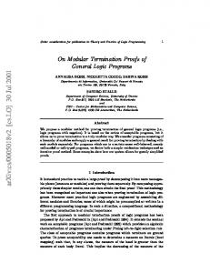
(3) A well-known problem with the standard SLDNF-tree approach (formally called SLDNF-resolution [Clark 1978; Lloyd 1987]) is that for some programs, such as P = {A ← ¬A} and G0 =← A, no SLDNF-trees exist [Apt and Doets 1994; Kunen 1989; Martelli and Tricomi 1992]. The main reason for this abnormality lies in the fact that to solve a negative subgoal ¬A it generates a subsidiary SLDNF-tree F T for P ∪ {← A} via R which is supposed either to contain a success leaf or to consist of failure leaves. When F T neither contains a success leaf nor finitely fails by going into an infinite derivation, the negative subgoal cannot be handled. In contrast, SLDNF∗ -trees exist for any general logic programs. A ground negative subgoal ¬A at a node Ni succeeds if all branches of the subsidiary SLDNF∗ -tree TNi+1 :←A end with a failure leaf (see the case 2(b)iii), and fails if TNi+1 :←A has a success leaf (see the case 2(b)i). Otherwise, the value of the subgoal ¬A is undetermined and thus Ni is marked as LAST, showing that it is the last node of the underlying SLDNF∗ -tree which can be finitely generated (see the case 2(b)iv).1 The tree is then completed here. For convenience, we use dotted edges “· · ·⊲′′ to connect parent and child (subsidiary) SLDNF∗ -trees, so that infinite derivations across SLDNF∗ -trees can be clearly identified. Formally, we have Definition 2.3. Let P be a general logic program, G0 a top goal and R the depthfirst, left-most control strategy. Let TN0 :G0 be the SLDNF∗ -tree for P ∪ {G0 } via R with ALA0 @N0 = ∅. A generalized SLDNF-tree for P ∪ {G0 } via R, denoted GTG0 , is rooted at N0 : G0 and consists of TN0 :G0 along with all its descendant SLDNF∗ -trees, where parent and child SLDNF∗ -trees are connected via “· · ·⊲′′ . Therefore, a path of a generalized SLDNF-tree may come across several SLDNF∗ trees through dotted edges. Any such a path starting at the root node N0 : G0 is called a generalized SLDNF-derivation. Thus, there may occur two types of edges in a generalized SLDNF-derivation, C “−→” and “ · · · ⊲′′ . For convenience, we use “ ⇒′′ to refer to either of them. Moreover, for any node Ni : Gi we use L1i to refer to the selected (i.e. left-most) subgoal in Gi . Example 2.1. Let P1 be a general logic program and G0 a top goal, given by P1 : G0 :

p(X) ← ¬p(f (X)). ← p(a).

Cp1

The generalized SLDNF-tree GT←p(a) for P1 ∪ {G0 } is shown in Figure 1, where ∞ represents an infinite extension. Note that to expand the node N1 , we build a 1 This case occurs when either T ∗ Ni+1 :←A or some of its descendant SLDNF -trees is infinite, or TNi+1 :←A has an infinite number of descendant SLDNF∗ -trees. Note that LAST is used here only for the purpose of formulating an SLDNF∗ -tree − showing that Ni is the last node of the SLDNF∗ -tree. In practical implementation of SLDNF∗ -trees, in such a case Ni will never be marked by LAST since it requires an infinitely long time to build TNi+1 :←A together with all of its descendant SLDNF∗ -trees. However, the SLDNF∗ -tree is always completed at Ni , whether Ni is marked by LAST or not, because (1) such a case occurs at most one time in an SLDNF∗ -tree and (2) it always occurs at the last generated node Ni .

ACM Transactions on Computational Logic, Vol. TBD, No. TBD, TBD 20TBD.

Characterizing Termination of General Logic Programs

·

7

subsidiary SLDNF∗ -tree TN2 :←p(f (a)) . Since TN2 :←p(f (a)) neither contains a success leaf nor finitely fails (i.e. not all of its leaf nodes are marked as ✷f ), N1 is the last node of TN0 :←p(a) , marked as LAST. We see that GT←p(a) is infinite, although all of its SLDNF∗ -trees are finite. N0 : ← p(a) Cp1

❄

N1 : ← ¬p(f (a))

✲ N2 : ← p(f (a))

. . . . .

Cp1

LAST

❄

N3 : ← ¬p(f (f (a)))

✲ N4 : ← p(f (f (a)))

. . . . .

Cp1

LAST

Fig. 1.

❄ ∞

The generalized SLDNF-tree GT←p(a) .

Example 2.2. Consider the following general logic program and top goal. p ← ¬q. q. q ← q. ← p.

P2 :

G0 :

Cp1 Cq1 Cq2

The generalized SLDNF-tree GT←p for P2 ∪{G0 } is depicted in Figure 2 (a). GT←p consists of two SLDNF∗ -trees, TN0 :←p and TN2 :←q , which are constructed as follows. Initially, TN0 :←p has only the root node N0 :← p. Expanding the root node against the clause Cp1 leads to the child node N1 :← ¬q. We then build a subsidiary SLDNF∗ -tree TN2 :←q for P2 ∪ {← q} via the depth-first, left-most control strategy, where the expansion stops right after the node N3 is marked as LAST. Since TN2 :←q has a success leaf, N1 gets a failure child node N5 . TN0 :←p is then completed. For the purpose of comparison, the standard SLDNF-trees for P2 ∪ {← p} are shown in Figure 2 (b). Note that Figure 2 (a) is finite, whereas Figure 2 (b) is not. N0 : ← p Cp1

❄

N1 : ← ¬q .

.

❏❏ ❫

. ✢ .

N5 : ✷f

N2 : ← q Cq1

✡ ✢✡

N3 : ✷t

C

q2 ❏❏ ❫

N2 : ← q

N0 : ← p

Cq1

Cp1

❄

✡ ✢✡ ❏❏ ❫Cq2

N3 : ✷t N4 : ← q

N1 : ← ¬q

✡ ✢✡ ❏❏ ❫Cq2 N5 : ✷t ∞ Cq1

❄ N∞ : ✷f

N4 : ← q

LAST

(a)

(b)

Fig. 2. The generalized SLDNF-tree GT←p (a) and its two corresponding standard SLDNF-trees (b).

ACM Transactions on Computational Logic, Vol. TBD, No. TBD, TBD 20TBD.

·

8

Yi-Dong Shen et al.

3. CHARACTERIZING AN INFINITE GENERALIZED SLDNF-DERIVATION In this section we establish a necessary and sufficient condition for an infinite generalized SLDNF-derivation. We begin by introducing a few concepts. Definition 3.1. Let T be a term or an atom and S be a string that consists of all predicate symbols, function symbols, constants and variables in T , which is obtained by reading these symbols sequentially from left to right. The symbol string of T , denoted ST , is the string S with every variable replaced by X . For instance, let T1 = a, T2 = f (X, g(X, f (a, Y ))) and T3 = [X, a]. Then ST1 = a, ST2 = f X gX f aX and ST3 = [X |[a|[]]]. Note that [X, a] is a simplified representation for the list [X|[a|[]]]. Definition 3.2. Let ST1 and ST2 be two symbol strings. ST1 is a projection of ST2 , denoted ST1 ⊆proj ST2 , if ST1 is obtained from ST2 by removing zero or more elements. For example, aX X bc ⊆proj f aX eX bX cd. It is easy to see that the relation ⊆proj is reflexive and transitive. That is, for any symbol strings S1 , S2 and S3 , we have S1 ⊆proj S1 , and that S1 ⊆proj S2 and S2 ⊆proj S3 implies S1 ⊆proj S3 . Definition 3.3. Let A1 = p(.) and A2 = p(.) be two atoms. A1 is said to loop into A2 , denoted A1 ❀loop A2 , if SA1 ⊆proj SA2 . Let Ni : Gi and Nj : Gj be two nodes in a generalized SLDNF-derivation with L1i ≺anc L1j and L1i ❀loop L1j . Then Gj is called a loop goal of Gi . The following result is immediate. Theorem 3.4. (1 ) The relation ❀loop is reflexive and transitive. (2 ) If A1 ❀loop A2 then |A1 | ≤ |A2 |. (3 ) If G3 is a loop goal of G2 that is a loop goal of G1 then G3 is a loop goal of G1 . Observe that since a logic program has only a finite number of clauses, an infinite generalized SLDNF-derivation results from repeatedly applying the same set of clauses, which leads to infinite repetition of selected variant subgoals or infinite repetition of selected subgoals with recursive increase in term size. By recursive increase of term size of a subgoal A from a subgoal B we mean that A is B with a few function/constant/variable symbols added and possibly with some variables changed to different variables. Such crucial dynamic characteristics of an infinite generalized SLDNF-derivation are captured by loop goals, as shown by the following principal theorem. Theorem 3.5. D is an infinite generalized SLDNF-derivation if and only if it is of the form N0 : G0 ⇒ ...Ng1 : Gg1 ⇒ ...Ng2 : Gg2 ⇒ ...Ng3 : Gg3 ⇒ ... such that for any j ≥ 1, Ggj+1 is a loop goal of Ggj . We need Higman’s Lemma to prove this theorem.2 2 It

is one of the anonymous reviewers who brought this lemma to our attention.

ACM Transactions on Computational Logic, Vol. TBD, No. TBD, TBD 20TBD.

Characterizing Termination of General Logic Programs

·

9

Lemma 3.6 (Higman’s Lemma [Higman 1952; Bol 1991]). Let {Ai }∞ i=1 be an infinite sequence of strings over a finite alphabet Σ. Then for some i and k > i, Ai ⊆proj Ak The following result follows from Lemma 3.6. Lemma 3.7. Let {Ai }∞ i=1 be an infinite sequence of strings over a finite alphabet Σ. Then there is an infinite increasing integer sequence {ni }∞ i=1 such that for all i Ani ⊆proj Ani+1 . Proof.

3

Suppose this is not true. Let us take a finite maximal subsequence An1 ⊆proj An2 ⊆proj ... ⊆proj Ank1

The subsequence is maximal in the sense that for no i > nk1 do we have Ank1 ⊆proj Ai . We know that such a subsequence with length at least 2 must exist from Lemma 3.6 and the assumption that the assertion of the lemma does not hold for the sequence {Ai }∞ i=1 . Now look at the elements of the original sequence with indices larger than nk1 and take another such finite maximal subsequence from them. Continuing in this way, we get infinitely many such maximal subsequences. Let {Anki }∞ i=1 be the sequence of last elements of the maximal subsequences. By Lemma 3.6, this sequence has two elements, Anki and Ankj with nki < nkj , such that Anki ⊆proj Ankj . This contradicts the assumption that Anki is the last element of some finite maximal subsequence. The following lemma is needed to prove Theorem 3.5. Lemma 3.8. Let D be an infinite generalized SLDNF-derivation. Then there are infinitely many goals Gg1 , Gg2 , ... in D such that for any j ≥ 1, L1j ≺anc L1j+1 . Proof. Let D be of the form N0 : G0 ⇒ N1 : G1 ⇒ ... ⇒ Ni : Gi ⇒ Ni+1 : Gi+1 ⇒ ... C

Consider derivation steps like Ni : Gi −→ Ni+1 : Gi+1 · · · ⊲Ni+2 : Gi+2 , where L1i is a positive subgoal and L1i+1 = ¬A a negative subgoal. So L1i+2 = A. We see that both L1i and L1i+1 need the proof of L1i+2 . Moreover, given L1i+2 the provability of L1i does not depend on L1i+1 . Since L1i+1 has no descendant subgoals, removing it would affect neither the provability nor the ancestor-descendant relationships of other subgoals in D. Therefore, we delete L1i+1 by marking Ni+1 with #. C

For each derivation step Ni : Gi −→ Ni+1 : Gi+1 , where L1i is a positive subgoal and C = A ← B1 , ...Bn such that Aθ = L1i θ under an mgu θ, we do the following: (1) If n = 0, which means L1i is proved at this step, mark node Ni with #. (2) Otherwise, the proof of L1i needs the proof of Bj θ (j = 1, ..., n). If all descendant nodes of Ni in D have been marked with #, which means that all Bj θ have been proved at some steps in D, mark node Ni with #. Note that the root node N0 will never be marked with #, for otherwise G0 would have been proved and D should have ended at a success or failure leaf. After the above marking process, let D become 3 This

proof is suggested by an anonymous reviewer. ACM Transactions on Computational Logic, Vol. TBD, No. TBD, TBD 20TBD.

10

·

Yi-Dong Shen et al.

N0 : G0 ⇒ ... ⇒ Ni1 : Gi1 ⇒ ... ⇒ Ni2 : Gi2 ⇒ ... ⇒ Nik : Gik ⇒ ... where all nodes except N0 , Ni1 , Ni2 , ..., Nik , ... are marked with #. Since we use the depth-first, left-most control strategy, for any j ≥ 0 the proof of L1ij needs the proof of L1ij+1 (let i0 = 0), for otherwise Nij would have been marked with #. That is, L1ij is an ancestor subgoal of L1ij+1 . Moreover, D must contain an infinite number of such nodes because if Nik : Gik was the last one, which means that all nodes after Nik were marked with #, then L1ik would be proved, so that Nik should be marked with #, a contradiction. We are ready to prove Theorem 3.5. Proof (Proof of Theorem 3.5). (⇐=) Straightforward. (=⇒) By Lemma 3.8, D contains an infinite sequence of selected subgoals H1 = 1 1 {L1ji }∞ i=1 such that for any i Lji ≺anc Lji+1 . Since any logic program has only a finite number of predicate symbols, H1 must have an infinite subsequence H2 = {L1ki }∞ i=1 such that all L1ki have the same predicate symbol, say p. We now show that H2 has 1 1 an infinite subsequence {L1gi }∞ i=1 such that for any i Lgi ❀loop Lgi+1 . Let T be the (finite) set of all constant and function symbols in the logic program and let Σ = T ∪{X }. Then the symbol string SL1k of each L1ki in H2 is a string over i Σ that begins with p. These symbol strings constitute an infinite sequence {pAi }∞ i=1 with each Ai being a substring. By Lemma 3.7 there is an infinite increasing integer sequence {ni }∞ i=1 such that for any i pAni ⊆proj pAni+1 . Therefore, H2 has an infinite subsequence H3 = {L1gi }∞ i=1 with SL1gi = pAni being the symbol string of L1gi . That is, for any i SL1g ⊆proj SL1g . Thus, for any i L1gi ❀loop L1gi+1 . i

i+1

4. CHARACTERIZING TERMINATION OF GENERAL LOGIC PROGRAMS In [Schreye and Decorte 1993], a generic definition of termination of logic programs is presented as follows. Definition 4.1 ([Schreye and Decorte 1993]). Let P be a general logic program, SQ a set of queries and SR a set of selection rules. P is terminating w.r.t. SQ and SR if for each query Qi in SQ and for each selection rule Rj in SR , all SLDNF-trees for P ∪ {← Qi } via Rj are finite. Observe that the above definition considers finite SLDNF-trees for termination. That is, P is terminating w.r.t. Qi only if all (complete) SLDNF-trees for P ∪ {← Qi } are finite. This does not seem to apply to Prolog where there exist cases in which P is terminating w.r.t. Qi and Rj , although some (complete) SLDNF-trees for P ∪ {← Qi } are infinite. Example 2.2 gives such an illustration, where Prolog terminates with a negative answer to the top goal G0 . In view of the above observation, we present the following slightly different definition of termination based on a generalized SLDNF-tree. Definition 4.2. Let P be a general logic program, SQ a finite set of queries and R the depth-first, left-most control strategy. P is terminating w.r.t. SQ and R if for each query Qi in SQ , the generalized SLDNF-tree for P ∪ {← Qi } via R is finite. The above definition implies that P is terminating w.r.t. SQ and R if and only if there is no infinite generalized SLDNF-derivation in any generalized SLDNF-tree ACM Transactions on Computational Logic, Vol. TBD, No. TBD, TBD 20TBD.

Characterizing Termination of General Logic Programs

·

11

GT←Qi . This obviously applies to Prolog. We then have the following immediate result from Theorem 3.5, which characterizes termination of a general logic program. Theorem 4.3. P is terminating w.r.t. SQ and R if and only if for each query Qi in SQ there is no generalized SLDNF-derivation in GT←Qi of the form N0 : G0 ⇒ ...Ng1 : Gg1 ⇒ ...Ng2 : Gg2 ⇒ ...Ng3 : Gg3 ⇒ ... such that for any j ≥ 1, Ggj+1 is a loop goal of Ggj . 5. RELATED WORK Concerning termination analysis, we refer the reader to the papers of Decorte, De Schreye and Vandecasteele [Schreye and Decorte 1993; Decorte et al. 1999] for a comprehensive bibliography. Most existing termination analysis techniques are static approaches, which only make use of the syntactic structure of the source code of a logic program to establish some well-founded conditions/constraints that, when satisfied, yield a termination proof. Since non-termination is caused by an infinite generalized SLDNF-derivation, which contains some essential dynamic characteristics that are hard to capture in a static way, static approaches appear to be less precise than a dynamic one. For example, it is difficult to apply a static approach to prove the termination of program P2 in Example 2.2 with respect to a query pattern p. The concept of generalized SLDNF-trees is the basis of our approach. There are several new definitions of SLDNF-trees presented in the literature, such as that of Apt and Doets [Apt and Doets 1994], Kunen [Kunen 1989], or Martelli and Tricomi [Martelli and Tricomi 1992]. Generalized SLDNF-trees have two distinct features as compared to these definitions. First, the ancester-descendent relation is explicitly expressed (using ancester lists) in a generalized SLDNF-tree, which is essential in identifying loop goals. Second, a ground negative subgoal ¬A at a node Ni in a SLDNF∗ -tree TNr :Gr is formulated in the same way as in Prolog, i.e. (1) the subsidiary SLDNF∗ -tree TNi+1 :←A for the subgoal terminates at the first success leaf, and (2) ¬A succeeds if all branches of TNi+1 :←A end with a failure leaf and fails if TNi+1 :←A has a success leaf. When TNi+1 :←A goes into an infinite extension, the node Ni is treated as the last node of TNr :Gr which can be finitely generated. As a result, a generalized SLDNF-tree exists for any general logic programs. Our work is also related to loop checking − another research topic in logic programming which focuses on detecting and eliminating infinite loops. Informally, a derivation N0 : G0 ⇒ N1 : G1 ⇒ ... ⇒ Ni : Gi ⇒ ... ⇒ Nk : Gk ⇒ ... is said to step into a loop at a node Nk : Gk if there is a node Ni : Gi (0 ≤ i < k) in the derivation such that Gi and Gk are sufficiently similar. Many mechanisms related to loop checking have been presented in the literature (e.g. [Bol et al. 1991; Shen et al. 2001]). However, most of them apply only to SLD-derivations for positive logic programs and thus cannot deal with infinite recursions through negation like that in Figure 1 or 2. Loop goals are defined on a generalized SLDNF-derivation for general logic programs and can be used to define the sufficiently similar goals in loop checking. For ACM Transactions on Computational Logic, Vol. TBD, No. TBD, TBD 20TBD.

12

·

Yi-Dong Shen et al.

such an application, they play a role similar to expanded variants defined in [Shen et al. 2001]. Informally, expanded variants are variants except that some terms may grow bigger. However, expanded variants have at least three disadvantages as compared to loop goals: their definition is less intuitive, their computation is more expensive, and they are not transitive in the sense that A being an expanded variant of B that is an expanded variant of C does not necessarily imply A is an expanded variant of C. 6. CONCLUSIONS AND FUTURE WORK We have presented an approach to characterizing termination of general logic programs by making use of dynamic features. A concept of generalized SLDNF-trees is introduced, a necessary and sufficient condition for infinite generalized SLDNFderivations is established, and a new characterization of termination of a general logic program is developed. We have recently developed an algorithm for automatically predicting termination of general logic programs based on the characterization established in this paper. The algorithm identifies the most-likely non-terminating programs. Let P be a general logic program, SQ a set of queries and R the depth-first, left-most control strategy. P is said to be most-likely non-terminating w.r.t. SQ and R if for some query Qi in SQ , there is a generalized SLDNF-derivation with a few (e.g. two or three) loop goals. Our experiments show that for most representative general logic programs we have collected in the literature, they are not terminating w.r.t. SQ and R if and only if they are most-likely non-terminating w.r.t. SQ and R. This algorithm can be incorporated into Prolog as a debugging tool, which would provide the users with valuable debugging information for them to understand the causes of non-termination. Tabled logic programming is receiving increasing attention in the community of logic programming (e.g. [Chen and Warren 1996; Shen et al. 2002]). Verbaeten, De Schreye and Sagonas [Verbaeten et al. 2001] recently exploited termination proofs for positive logic programs with tabling. For future research, we are considering extending the work of the current paper to deal with general logic programs with tabling. ACKNOWLEDGMENTS

We are particularly grateful to Danny De Schreye, Krzysztof Apt, Jan Willem Klop and the three anonymous referees for their constructive comments on our work and valuable suggestions for its improvement. One anonymous reviewer brought the Higman’s lemma to our attention. Another anonymous reviewer suggested the proof of Lemma 3.7 and presented us a different yet interesting proof to the Higman’s lemma based on an idea from Dershowitz’s paper [Dershowitz 1987]. The work of Yi-Dong Shen is supported in part by Chinese National Natural Science Foundation and Trans-Century Training Program Foundation for the Talents by the Chinese Ministry of Education. Qiang Yang is supported by NSERC and IRIS III grants. REFERENCES Apt, K. R. and Doets, K. 1994. A new definition of sldnf-resolution. Journal of Logic Programming 18, 177–190. ACM Transactions on Computational Logic, Vol. TBD, No. TBD, TBD 20TBD.

Characterizing Termination of General Logic Programs

·

13

Apt, K. R. and Pedreschi, D. 1993. Reasoning about termination of pure prolog programs. Information and Computation 106, 109–157. Bezem, M. 1992. Characterizing termination of logic programs with level mapping. Journal of Logic Programming 15, 1/2, 79–98. Bol, R. N. 1991. Loop checking in logic programming. Ph.D. thesis, The University of Amsterdam, Amsterdam. Bol, R. N., Apt, K. R., and Klop, J. W. 1991. An analysis of loop checking mechanisms for logic programs. Theoretical Computer Science 86, 1, 35–79. Bossi, A., Cocco, N., and Fabris, M. 1994. Norms on terms and their use in proving universal termination of a logic program. Theoretical Computer Science 124, 1, 297–328. Brodsky, A. and Sagiv, Y. 1991. Inference of inequality constraints in logic programs. In Proceedings of the Tenth ACM SIGACT-SIGMOD-SIGART Symposium on Principles of Database Systems. ACM Press, Denver, 227–240. Chan, D. 1988. Constructive negation based on the completed database. In Proceedings of the Fifth International Conference and Symposium on Logic Programming. MIT Press, Seattle, 111–125. Chen, W. D. and Warren, D. S. 1996. Tabled evaluation with delaying for general logic programs. J. ACM 43, 1, 20–74. Clark, K. L. 1978. Negation as failure. In (H.Gallaire and J. Minker, eds.) Logic and Databases. Plenum, New York, 293–322. Decorte, S., Schreye, D. D., and Fabris, M. 1993. Automatic inference of norms: A missing link in automatic termination analysis. In Proceedings of the 1993 International Symposium on Logic Programming. MIT Press, Vancouver, Canada, 420–436. Decorte, S., Schreye, D. D., and Vandecasteele, H. 1999. Constraint-based termination analysis of logic programs. ACM Transactions on Programming Languages and Systems 21, 6, 1137–1195. Dershowitz, N. 1987. Termination of rewriting. J. Symbolic Computation 3, 69–116. Higman, G. 1952. Ordering by divisibility in abstract algebras. Proceedings of the London Mathematical Society 3, 2, 326–336. ISLAB. 1998. SICStus Prolog User’s Manual. Intelligent Systems Laboratory, Swedish Institute of Computer Science, Available from http://www.sics.se/sicstus/docs/3.7.1/html/sicstus toc.html. Kunen, K. 1989. Signed data dependencies in logic programming. Journal of Logic Programming 7, 231–246. Lindenstrauss, N. and Sagiv, Y. 1997. Automatic termination analysis of logic programs. In Proceedings of the Fourteenth International Conference on Logic Programming. MIT Press, Leuven, Belgium, 63–77. Lloyd, J. W. 1987. Foundations of Logic Programming. Springer-Verlag, Berlin. Martelli, M. and Tricomi, C. 1992. A new sldnf-tree. Information Processing Letters 43, 2, 57–62. Martin, J. C., King, A., and Soper, P. 1997. Typed norms for typed logic programs. In Proceedings of the 6th International Workshop on Logic Programming Synthesis and Transformation. Springer, Stockholm, Sweden, 224–238. Plumer, L. 1990a. Termination Proofs for Logic Programs. Lecture Notes in Computer Science 446, Springer-Verlag, Berlin. Plumer, L. 1990b. Termination proofs for logic programs based on predicate inequalities. In Proceedings of the Seventh International Conference on Logic Programming. MIT Press, Cambridge, MA, 634–648. Schreye, D. D. and Decorte, S. 1993. Termination of logic programs: the never-ending story. Journal of Logic Programming 19, 20, 199–260. Schreye, D. D. and Verschaetse, K. 1995. Deriving linear size relations for logic programs by abstract interpretation. New Generation Computing 13, 2, 117–154. ACM Transactions on Computational Logic, Vol. TBD, No. TBD, TBD 20TBD.

14

·

Yi-Dong Shen et al.

Schreye, D. D., Verschaetse, K., and Bruynooghe, M. 1992. A framework for analyzing the termination of definite logic programs with respect to call patterns. In Proceedings of the International Conference on Fifth Generation Computer Systems. IOS Press, Tokyo, Japan, 481–488. Shen, Y. D., Yuan, L. Y., and You, J. H. 2001. Loop checks for logic programs with functions. Theoretical Computer Science 266, 1/2, 441–461. Shen, Y. D., Yuan, L. Y., and You, J. H. 2002. Slt-resolution for the well-founded semantics. Journal of Automated Reasoning 28, 1, 53–97. Ullman, J. D. and Gelder, A. V. 1988. Efficient tests for top-down termination of logical rules. J. ACM 35, 2, 345–373. Verbaeten, S., Schreye, D. D., and Sagonas, K. 2001. Termination proofs for logic programs with tabling. ACM Transactions on Computational Logic 2, 1, 57–92. Verschaetse, K. 1992. Static termination analysis for definite horn clause programs. Ph.D. thesis, Department of Computer Science, K. U. Leuven, Available at http://www.cs.kuleuven.ac.be/ lpai.

Received June 2000; revised August 2001 and December 2001; accepted April 2002

ACM Transactions on Computational Logic, Vol. TBD, No. TBD, TBD 20TBD.