A Dynamic Programming Framework for Using

A Dynamic Programming Framework for Using Weather Derivatives to Manage Dairy Profit Risk

Gang Chen and Matthew C. Roberts∗ Department of Agricultural, Environmental, and Development Economics The Ohio State University 2120 Fyffe Road Columbus, Ohio 43210 Contact: [email protected]

Selected Paper prepared for presentation at the American Agricultural Economics Association Annual Meeting, Denver, Colorado, August 1-4, 2004

Copyright 2004 by Gang Chen and Matthew C. Roberts. All rights reserved. Readers may make verbatim copies of this document for non-commercial purposes by any means, provided that this copyright notice appears on all such copies.

∗ Graduate

Research Assistant and Assistant Professor, Department of Agricultural, Environmental, and Development Economics, The Ohio State University, Columbus, OH 43210. We thank Normand R. St-Pierre for his comments and suggestions.

A Dynamic Programming Framework for Using Weather Derivatives to Manage Dairy Profit Risk Abstract Dairy farms confront unique risks from weather conditions. Hot and humid weather induces heat stress, which reduces both the quantity and quality of dairy production. Traditional heat abatement technologies control the environment through ventilation, misting or evaporative cooling. Adoption of abatement equipment, however, is hindered by its high initial cost and possibly long payback period, especially for small- and medium-scale firms. Moreover, the abatement equipment is only seasonally useful as a fixed asset whose price rises with efficacy. Weather derivatives provide an alternative method of dairy farmers’ risk management. Since abatement equipment can be used for many years once installed, and its maintenance costs will increase and efficacy will decrease with age, a decision that must regularly be made by a dairy farmer is when to maintain his abatement equipment and when to replace it with a new one. The decision affects both current and expected future revenues. Considering that weather derivatives can be purchased periodically, the objective of this study is twofold: first, to test the risk management value of weather derivatives for dairy plant operations; second, to examine how weather derivatives can affect dairy producers’ abatement equipment decisions. In this study, we employ a dynamic programming framework to study the case that a representative dairy farmer maximizes his long-run utility using weather derivatives and abatement equipment. Keywords: abatement technology, dynamic programming, mean-variance efficiency, profit risk, weather derivatives

Introduction Dairy farms confront unique risks from weather conditions. Hot and humid weather induces heat stress, which reduces both the quantity and quality of dairy production (Barth; Thompson). Heat stress is measured by temperature-humidity index (THI, also commonly known as the ‘heat index’). Traditional heat abatement technologies control the environment through ventilation, misting or evaporative cooling. Adoption of abatement equipment, however, is hindered by its high initial cost and possibly long payback period, especially for small- and medium-scale firms. Moreover, the abatement equipment is only seasonally useful as a fixed asset whose price rises with efficacy. Weather derivatives provide an alternative method of dairy farmers’ risk management. Instead of reducing production losses, weather derivatives make payments based upon observed weather conditions over a period of time so that they offer the potential to offset profit losses caused by adverse weather events. Investment in abatement equipment is both irreversible1 and deferrable.2 So keeping the money on hand and deferring the investment is similar to keeping an American call option. These irreversible investment opportunities are typically called real options. They are valuable and the value is highly sensitive to the uncertainty of future cash flow of the investment. Once a farmer has made an investment in abatement equipment, the real option has been exercised and he gives up the possibility of waiting for new information to arrive that might affect the desirability or timing of the investment expenditure.3 The value of the real option is an opportunity cost that must be included as part of the investment cost. So whether or not to investment will not only depend on whether the Net Present Value (NPV) of a unit of capital is positive, but also whether the positive NPV is larger than the value of the real option. Pindyck (1991) shows that this kind of investment decision making problem under ir1 Due

to, for example, prohibitively high sunk cost, the “lemons” problem or that the investment is firmspecific. 2 “There may be a cost to delay - the risk of entry by other firms, or simply foregone cash flows - but this cost must be weighed against the benefits of waiting for new information.” pp. 1111, Pindyck (1991). 3 For example, see McDonald and Siegel (1986).

1

reversibility and uncertainty can be solved by using two qualitatively equivalent approaches: option pricing and dynamic programming. Since abatement equipment can be used for many years once installed,4 and its maintenance costs will increase and efficacy will decrease with age, a decision that must regularly be made by a dairy farmer is when to maintain his abatement equipment and when to replace it with a new one. The decision affects both current and expected future revenues. Many similar problems have been studied by using dynamic programming models in the literature. Examples include dairy cow replacement (Smith, 1972; Miranda and Schnitkey 1995), swine production (Chavas et al., 1985), poultry production (McClelland et al., 1989), livestock feeding (Burt, 1993), and bus engine replacement (Rust, 1987). Considering that weather derivatives can be purchased periodically, the objective of this study is twofold: first, to test the risk management value of weather derivatives for dairy plant operations; second, to examine how weather derivatives can affect dairy producers’ abatement equipment decisions. Dynamic programming approach is employed to determine the optimal actions to abatement equipment and optimal weather derivatives purchase. Specifically, we employ a dynamic programming framework to study the case that a representative dairy farmer maximizes his long-run utility using weather derivatives and abatement equipment. The actions that the dairy farmer need to determine at the start of each period include weather derivatives purchase amount and a choice from three alternative treatments to abatement equipment – no action, replacement, or maintenance, based upon the abatement equipment age and its maintenance history. A solution as the optimal risk management strategy for abatement equipment replacement and weather derivatives purchase is derived using policy iteration method. The empirical analysis is performed using 35-year daily weather data from Summit County and Cleveland, Ohio. The results suggest that simultaneously using weather derivatives and 4 Abatement

equipment typically has a lifespan of 7-10 years depending on the maintenances.

2

abatement technologies will outperform using abatement technologies alone, even in presence of basis risk and transaction costs. Thus weather derivatives expand the portfolio choice set, and make more desirable profit distributions available. Moreover, using weather derivatives will reduce the initial investment in abatement equipment and postpone the asset replacement, which mitigates the problem of high initial installation cost of abatement equipment for small- and medium-size firms.

Background Weather derivatives as relatively new financial products possess several unique properties distinguishing them from other derivatives. First, their underlying (i.e. weather) is not a tradable asset. Second, they hedge against volumetric risk instead of price risk. The indemnity is calculated based on a weather index (Cooling/Heating Degree-Days, rainfall, etc) rather than asset price. Third, they are not as liquid as traditional standard derivatives. If we assume away transaction costs, the traditional financial derivative markets are liquid. Weather, by its nature, is location-specific. Different locations have different weather conditions whether at the same time or across time. Due to their properties, weather derivatives have advantages over traditional financial derivatives in the view of hedging against weather risk. Because there is no need to prove damage to claim payoffs, there is little moral hazard. Furthermore, as weather information is almost perfectly symmetric, adverse selection is eliminated. At the same time, the use of weather derivatives is accompanied by basis risk caused by the fact that an end-user’s location often is not the same location as the reference location of the weather derivatives he holds. Economic losses are induced in the dairy industry when effective temperature conditions are out of dairy cows’ thermal comfort zone. According to St-Pierre, Cobanov and Schnitkey (SCS, 2003), heat stress in dairy cattle is a function of the Temperature-Humidity Index (THI). Johnson (1980) reports that a THI higher than 72 degrees is likely to have adverse ef3

fects on per-cow yield. In SCS, it is suggested that the threshold of THI to trigger heat stress should be lowered to 70 degrees accounting for the lower heat tolerance of the current selection of dairy cows. So 70 degrees is used as a threshold for risk from heat stress, THI threshold . According to the National Oceanic Atmospheric Administration (NOAA, 1976), the standard formula of THI is: THI = T – (0.55 – 0.55 RH) (T – 58), where T is temperature in degrees Fahrenheit and RH is relative humidity in percent. Since RH is is expressed as a percentage, it is easy to see that THI is positively correlated with temperature. THI is varying in a day along with change of temperature and relative humidity. The maximum THI is in the afternoon, when the temperature is highest and relative humidity is lowest; and the minimum THI is in the night, when the temperature is lowest and relative humidity is highest. In this paper, daily THI refers to daily maximum THI. If maximum THI is lower than 70 degrees in a day, there is no heat stress for dairy cows.

One-period Setting In a one-period setting, we develop a representative dairy farmer’s net profit model with using weather derivatives and abatement equipment to reduce the profit risk induced by heat stress. And in next section, this one-period profit function will be used in dynamic programming analysis for determining optimal sequential risk management strategies. To reduce the visual complexity, we drop the time subscripts of model notations in this section. Consider a dairy farmer who produces without using abatement equipment or weather e − T C, where P is milk price, Q e is the stochastic yield, derivatives. His profit is ye = P · Q and T C denotes a total cost. For analytical simplicity, it is assumed there is no price risk; therefore price is normalized to unity. The tilde (e ) denotes a random variable. Suppose expected profit of a farmer is his historical average, µ, so the difference between ye and µ is his profit risk. The profit risk is orthogonally decomposed into two parts. One

4

is systematic risk which comes from weather conditions; the other is nonsystematic risk which reflects the individual’s production variability not arising from weather and is assumed uncorrelated with weather conditions. Equations (1)-(10) give the daily models, because equation (3), by its nature, is for daily calculation. However, they can be easily transformed into yearly models by using yearly cumulative values of the variables. ye = µ + θ · f (e x) + εe,

(1) where (2)

e = E(e x z ) − ze

(3)

g − THI threshold , 0) ze = max(THI θ = cov(e y , f (e x))/var(f (e x))

(4)

E(e y ) = µ, E(e ε) = 0, var(e ε) = σεe2 , cov(e z , εe) = 0, cov(e x, εe) = 0.

(5)

The coefficient θ quantifies the sensitivity of the farmer’s individual profit to systematic risk. The factor ze, which is common to all producers in a region, measures the degree of e denotes the weather condition compared to its expectation. If heat stress, and the factor x e ze is lower than E(e z ), it means the heat stress is milder than its expectation. In this case, x e. The functional form of is positive. And f (e x) captures systematic risk and increases with x f (e x) is assumed to be linear, i.e. f (e x) = α· x e, where α is a positive parameter of the linear relationship. The final term εe is a nonsystematic risk component. Then equation (1) becomes, (6)

ye = µ + θ · α · x e + εe = µ + β · x e + εe

where (7)

e)/ var(e β = cov(e y, x x).

5

Suppose that weather derivatives are available for purchase. Since here the risk is from excessively high THI, weather derivatives that will be used are focused on weather call opg and the strike price is THI threshold . The payoff from a tions. The underlying index is THI, weather call option is: g − THI threshold , 0) = ze. e = max(THI n

(8)

The hypothetical5 option premium is calculated on the basis of actuarial fairness. So purchasing weather options cannot change the farmer’s farmer’s expected profit. The option premium equals the expected payoff: π = E(e n) = E(e z ).

(9)

The timing of using weather derivatives is as follows: at the start of the period, the farmer buys weather derivatives; then at the end of the period, when all the weather information of this period has been observed, the farmer receives payoff (if any) from weather derivatives. Also suppose that the producer is free to choose his abatement equipment investment and maintenance strategy. By using abatement equipment, the production loss from heat stress can be reduced. The biological effectiveness of abatement equipment is a function of its e denote the reduced profit initial investment, age, maintenance, and weather condition. Let m loss, i.e. the increased profit from using abatement equipment; and let λ denote the costs of abatement equipment operating strategy. The explicit functional form will be given in the next section. Thus with weather options and abatement equipment, the producer’s net profit equals: (10)

yenet = ye + φ · (e n − π) + m e −λ

where φ is weather options purchase amount. Therefore, there are two elements that the 5 There

has not been a weather derivative on THI in the security market yet.

6

producer need to determine: weather options purchase amount and abatement equipment operating strategy.

Dynamic Programming Model This section presents a theoretical model of analyzing an asset replacement problem and examining how weather derivatives will affect the decisions. The assumptions include that first and second moments of accumulated weather conditions are constant and a representative farmer has mean-variance utility form. Thus the abatement investment and operating strategy will not depend on the current weather conditions, instead it will depend on the first and second moments of weather conditions. Suppose a representative dairy farmer is seeking an optimal risk management strategy with the aim to maximize the present value of his long-run utility. Since abatement equipment is a kind of fixed asset, its investment level cannot be changed once installed. So the farmer need to decide the lump-sum initial installation investment. Then at the beginning of every following year, he observes the state, i.e. the status of his abatement equipment: (i) its age, and (ii) how many years since last maintenance – the state information affects the effectiveness of abatement equipment. Then the farmer needs to determine: (i) which action to take for his abatement equipment in three alternative choices: no action, replacement, and service, and (ii) weather derivatives purchase amount. Formally, the representative farmer’s decision problem is written as:

∞

(11)

max ∑ δ t U (st , xt ) t=0

where t is time index in calendar year; δ ∈ (0, 1) is the farmer’s discount factor reflecting interest rate and the individual’s impatience; U (st , xt ) is utility of year t; st is a vector of state

7

variables at t; and xt is the farmer’s decisions at t. This is an infinite horizon, deterministic model. More explicitly, the discrete time dynamic programming model consists of the following objects: a state space, an action space, transition rule, a utility function, and a discount factor δ. We now turn to the detailed description of the model.

State and Action Variables

The state vector st = (at , ht ) consists of two variables: at = {1, 2, ..., lifespan}: age of abatement equipment; ht = {1, 2, ..., lifespan}: maintenance history (i.e. how many years since last maintenance). The state variables, observed at the start of period t, represent the abatement equipment’s current status that affects its effectiveness and maintenance costs in period t. And  the action vector xt = (it , φt ) also consists of two variables:   1, no action    it = 2, maintenance      3, replace is abatement equipment operating decision at time t; φt ∈ R+ : weather derivatives purchase amount at time t. Once observing the state values, the farmer’s decision problem is to choose the abatement equipment operating action, which will affect the current and future utility; and weather derivatives purchase amount, which will only affect utility of period t since the payoff (if any) will be claimed at the end of that period. The abatement status transition function is:

8

   (at + 1, ht + 1),    (at+1 , ht+1 ) = (at + 1, 1),      (1, 1),

if it = 1 (no action) if it = 2 (maintenance) if it = 3 (replace) .

Formulating Profit and Utility Functions

In the one-period setting, net profit is given by: (12)

yetnet = yet + φt · (e nt − π) + m e t − λt ,

et + εet and π = E(e where yet = µ + β · x nt ). In (12), the biological functional form of the effectiveness of abatement equipment is formulated as: (13)

g t )√η] , e t = κ(ht +at /n) [(b + c · THI m

where m e t is the reduced profit loss, i.e. the increased profit from using abatement equipment; g t is cumulative THI of period t; η is initial abatement equipment installation investment; THI κ ∈ (0, 1) reflects the declining effectiveness with aging and less frequent maintenance; and b and c are parameters reflecting the effect of weather condition. Suppose that the producer is free to choose his initial abatement equipment investment η ( η ≥ 0 ; and η = 0 means he does not install abatement equipment). It is easy to see that gt . When η = 0, m e t is increasing with η and THI e t is also equal to 0. And with fixed η, m et m g t . That is because although the profit is low when THI g t is high, the is increasing with THI reduced profit loss will be high with using abatement equipment; on the other hand, when g t is low (i.e. weather is good in period t), the abatement equipment is not of much use, THI so the reduced loss is low. Thus the parameter c is positive.

9

In (12), the costs of abatement equipment operating strategy, λt are specified as:    0, it = 1    (14) λt = (k1 at + k2 ht ) · η, it = 2      η, it = 3 . Here, k1 and k2 are positive parameters. So maintenance costs are increasing with age at and maintenance history ht . Replacement costs are equal to initial abatement investment by assuming the residual value of the old equipment equals its uninstall costs. In summary, the profit function is specified as:   g t )√η],  yet + φt · (e nt − π) + κ(ht +at /n) [(b + c · THI it = 1    g t )√η] − (k1 at + k2 ht ), it = 2 (15) yetnet = yet + φt · (e nt − π) + κ(at /n) [(b + c · THI      yet + φt · (e g t )√η] − η, nt − π) + [(b + c · THI it = 3 . Note that at the beginning of a period, if the farmer chooses to replace his abatement equipment with a new one, at and ht turn to zero in that period; if he chooses to have maintenance service, ht turns to zero in that period. The producer is assumed to have a mean-variance utility function6 of 1 U = E(•) − A · var(•) 2

(16)

where A is an index of agents’ aversion to taking on risk. Then the representative producer’s objective is to choose initial abatement investment η, optimal option purchase φt , and abatement equipment operating strategy it to maximize his long-run utility:

∞

(17)

∞

1

ytnet )] . δ Ut ≡ max ∑ δ t [E(e ytnet ) − A · var(e ∑ 2 η,φt ,it η,φt ,it max

t=0

t

t=0

6 This

framework is equivalent to expected utility maximization if (net) profit is distributed normally and producers’ utility function is exponential. But Meyer has shown that the mean-variance model is consistent with expected utility model under much weaker restrictions. See Pratt (1964) and Meyer (1987).

10

Thus far, the dynamic risk management problem is summarized by equations (15) and (17). In order to examine how weather derivatives will affect the decisions, we will compare the optimization solutions of the cases with and without using weather derivatives. Then the next task is to find the solution to this dynamic optimization problem.

Deriving Optimization Solution We first derive the optimal weather options purchase within one period setting taking the state and action variables as given. Then a dynamic programming problem across periods will be solved numerically. And the optimal initial abatement investment is chosen by examining a series of different investment levels and picking up the one with maximum Bellman value.

Optimization Within One Period

Because weather derivatives purchase amount in each period will only affect utility at that period and will not affect state variables, the optimal weather derivatives purchase, φt , can be decided within one period setting.

1 max Ut = max[E(e ytnet ) − A · var(e ytnet )] . 2 φt φt

(18) Specifically, (19)

1 Ut = E(e yt ) + φt E(e nt − π) + E(m e t − λt ) − A · [var(e yt ) + φ2t var(e nt ) 2 +var(m e t ) + 2φt cov(e yt , n et ) + 2cov(e yt , m e t ) + 2φt cov(e nt , m e t )] 1 √ 2 2 2 2 2 = µ + κ(ht +at /n) (b + cµTHI n g ) η − λt − A · [β σze + σεe + φt σn e − 2βφt σze,e 2 √ (ht +at /n) 2 (ht +at /n) √ φt c ησTHI,e +κ(2ht +2at /n) c2 ησTHI c ησTHI,e g z + 2κ g n] g − 2βκ

11

2 g g t ); σze,en = where µ = E(e yt ), µTHI zt ), σne2 = var(e nt ), σ 2g = var(THI g = E(THI t ); σze = var(e THI

g et ), σ g = cov(THI g t, n et ), σTHI,e et ). From equation (9), we know that cov(e zt , n g z = cov(THI t , z THI,e n et = zet . Therefor σne2 = σze2 = σze,en and σTHI,e n g z = σTHI,e g n . And all these are positive numbers. Take first order condition with respect to φt , (20)

√ φt σne2 − βσze,en + κ(ht +at /n) c ησTHI,e g n = 0.

From (20), the optimal weather options purchase amount is (21)

φ∗t = β − κ(ht +at /n) c

σTHI,e g z√ σze2

η.

The following three propositions are derived from equation (21): Proposition 1 . The optimal option purchase amount is increasing with β. It means that the more the producer’s profit is sensitive to weather risk, the more options he should purchase, ceteris paribus. Proposition 2 . The optimal weather option purchase amount is decreasing with initial abatement equipment investment η. Thus it indicates that weather options can act as a substitute for abatement equipment. Proposition 3 . The optimal weather options purchase amount is increasing with age at and maintenance history ht .

Propositions 2 and 3 say, for the best risk management results, if the farmer’s initial abatement investment is relatively low or the abatement equipment is old and less-frequently maintained, he should buy more weather options to hedge against risk from excessive heat stress.

Optimization Across Periods

Except in rare and highly specialized cases, it is impossible to derive analytical solution for dynamic programming problems. Here we employ numerical method to find the optimization 12

solution. The Bellman’s “principle of optimality” formally is expressed in the form of Bellman’s equation:

(22)

V (at , ht ) =

max {U (at , ht ; φt , it ) + δV (at+1 , ht+1 )}

φt ∈R+ ; it ∈{1,2,3}

where the Bellman value, V (at , ht ), is the maximum discounted sum of current and future utility starting from period t. Because the dynamic problem has an infinite horizon, the value function in equation (22) will not depend on time t.7 We may drop the time subscripts for the sake of visual clearness. Let v and x denote the vectors of Bellman values and optimal decisions corresponding to all possible states. And the Bellman’s equation is rewritten as a vector fixed-point equation: (23)

v = max {u(x) + δv} . x

The fixed-point equation can be solved to obtain unique and exact v and x by the policy iteration method. Specifically, the policy iteration algorithm consists of two steps: policy evaluation and policy improvement. Suppose that at iteration j, we have candidate decision rule xj . Then the value function vj can be recovered via policy evaluation, i.e. (24)

vj = {u(xj ) + δvj } = (1 − δ)−1 u(xj ) .

Next, at iteration j + 1, with xj and vj , a new policy xj+1 is formed via a policy improvement step: (25)

xj+1 = arg max{u(xj ) + δvj } .

7 Our

empirical analysis shows that there is not an obvious difference in optimal decisions and Bellman values between problems of infinite horizon and of a long finite horizon (say, 40 years), because after these many years the present discounted value of future utility is negligible.

13

Then xj+1 is put into equation (24) to update the Bellman’s value. The loop of (24) and (25) will be iterated until it converges. Therefore, the policy iteration algorithm converts the dynamic programming problem into the problem of computing a fixed point to a certain contraction mapping. The contraction property guarantees that the unique fixed point solution exists and is insensitive to rounding errors as long as discount rate δ is less than 1.

Basis Risk and Transaction Costs Basis risk exists in incomplete risk-world markets. Basis risk in this study comes from the difference between the underlying index of weather derivatives and the weather factor that affects the dairy profit (namely, THI). Two kinds of basis risk are investigated. One is geographical basis risk, which occurs from the difference in location between the reference site of weather derivatives and the actual production area. The other is reference-index basis risk, which occurs because weather derivatives are typically based upon temperature, yet biological stresses occur as a function of THI. Accordingly, the payoff from a weather call option, equation (8), is changed into: (26)

e = max(Ie− Ithreshold , 0) n

where Ie is the stochastic value of a weather index, and Ithreshold is the strike level. Equation (26) captures the presence of both reference-index and geographical basis risk. If the reference index Ie is temperature rather than THI, it reflects index basis risk. If the reference index Ie is weather condition of a location other than the production area, then geographical basis risk exists. Note that if Ie is THI of the production area, there is no basis risk. Transaction costs in weather options are imposed by setting the option premium as the expected payoff plus proportional transaction costs. Then equation (9) is revised into: (27)

π = (1 + γ)E(e n)

14

where the loading rate γ > 0 reflects transaction costs related to administrative and implementation fees and the desirability to the issuers. If γ is zero, the weather options are actuariallyfairly priced. The presence of basis risk and transaction costs changes the optimal weather derivatives purchase amount, i.e. equation (21), into: (28)

φ∗t = −

σg n √ σze,en γµne (ht +at /n) THI,e + β − κ c η. Aσne2 σne2 σne2

Propositions 1-3 still hold in equation (28). In addition, equation (28) shows that the optimal weather derivative purchase amount is negatively related to the loading rate γ. The intuition is that due to transaction costs, purchasing weather derivatives lowers expected profit, and thus higher transaction costs make weather derivatives less attractive.

Risk Management Effectiveness In order to derive the increased utility from using weather options and abatement equipment, we define the utility with using none of these two instruments as a benchmark. 1 Ut0 = E(e yt ) − A · var(e yt ) , 2

(29)

And the increased utility in certainty equivalent at t is: (30)

∆Ut = Ut − Ut0 1 = [E(e ytnet ) − E(e yt )] − A · [var(e ytnet ) − var(e yt )] . 2

Clearly, the optimal decision rule satisfies: ∞

(31)

∞

arg max{ ∑ δ t Ut } ≡ arg max( ∑ δ t ∆Ut ) . η,φt ,it

η,φt ,it

t=0

t=0

It is also viable to study the cases in which only one of the two instruments is used by 15

imposing the value of the other instrument to be zero. Therefore, risk management value of weather derivatives can be examined by comparing the cases of using both two instruments and using abatement equipment alone.

Data For the empirical illustration, we use 35-year (1949 to 1964 and 1984 to 2002) weather data of Summit County and Cleveland, Ohio collected from the National Climate Data Center (NCDC), a subsidiary of the National Oceanic Atmospheric Administration (NOAA).8 Summit County is treated as the real production area. And Cleveland, as a metropolitan city in the same state as the production area, is selected as the weather derivatives reference city for the purpose of investigating the effect of basis risk. The weather data include daily maximum and minimum temperature and daily maximum and minimum relative humidity. Daily temperature and dew point9 both follow routinely seasonal patterns each year. So the “burn-rate” method works well with them for pricing weather options. Daily maximum temperature-humidity index (THI) can be derived from g daily maximum temperature and minimum relative humidity.10 Note in the models, THI corresponds to maximum THI. When maximum THI is lower than 70 degrees in a day, there is no heat stress for dairy cows. Corresponding to the weather data of Summit County, a representative producer’s milk loss from heat stress and reduced loss from using abatement equipment are generated by employing the results in SCS.11 Abatement investment cannot change in a relatively long 8 It

is a quite common phenomenon that daily relative humidity data from 1965 to 1983 are missing across weather stations in NCDC database. 9 Dew point measures how much water vapor is in the air. In many places, the air’s total vapor content varies only slightly during an entire day, and so it is the changing air temperature that primarily regulates the full variation in relative humidity. Related information can be found at: http://www.usatoday.com/weather . 10 In a day, the maximum THI is in the afternoon, when the temperature is highest and relative humidity is lowest; and the minimum THI is in the night, when the temperature is lowest and relative humidity is highest. 11 See the Appendix for detail.

16

period once fixed. Also weather options are assumed to be written on summer basis, i.e. the e of a summer. Thus, Equations (6) and (13) will be estimated based payoff is cumulative n on cumulative summer data. The summer period is set from May 1st to Oct. 31st every year, because 97% of heat stress occurs in this period.

Empirical Illustration Note that all results of the empirical illustration in this paper is for one dairy cow, namely, the herd size is normalized into unity. We need values of the parameters in the models in order to solve the dynamic programming problem. Some of the parameters can be estimated from our data. Unfortunately, others such as the abatement maintenance cost parameters cannot be estimated due to lack of data. As a reference point for the empirical illustration, a base set of parameter values which cannot be estimated is established based upon discussions with experienced people and reasonable calibrations. Deviations from the base values provide insight into how changes in abatement equipment parameters and investors’ preference affect the risk management strategies and their corresponding results. A more favorable case would be to have data of dairy farmers’ abatement maintenance and replacement records, and effectiveness of abatement equipment in different states. Assuming the farmers’ asset maintenance/replacement decisions coincide with the dynamic optimization principle, several alternative functional forms of abatement effectiveness and maintenance costs can then be estimated and tested. With the estimated parameters, the optimal dynamic decision with simultaneously using weather derivatives and abatement equipment can be given. Table 1 gives the summary of the parameters, which are either estimated from our data or assigned. By and large, the empirical part of this paper is to provide an illustration on

17

how weather derivatives can be used together with abatement equipment to enhance a dairy farmer’s risk management effectiveness.

Parameter Estimation

Following SCS, THI threshold is set as 70 degrees. From the weather data of Summit County and the SCS milk loss model, we calculate the daily milk loss during summers of the 35 years g Then by accumulating the milk loss and ze = max(THI g− and the corresponding daily THI. THI threshold , 0) during each summer in the 35 years, we have 35 observations of cumulative profit loss and x e = E(e z ) − ze. From a least squares regression, β is estimated, which is 0.5635 kg milk per cow with Student’s t-value and R-squared of 16.47 and 0.89. That is to say each degree of ze beyond its mean will induce 0.5635 kg milk loss. The milk price is set as $ e. 0.287/kg as in SCS, so the milk loss is $ 0.1617 per degree of x We put the daily summer weather data into the SCS abatement effect model12 to calculate the daily reduced THI corresponding to seven abatement levels. Because the abatement levels in SCS are expressed as yearly investment with an annualization rate of 15%, we calibrate these levels into initial abatement investment levels η with the assigned parameters κ and n in equation (13) and with the assumption that the states of equipment in SCS is at = 6 and ht =0, or at = 2 and ht = 1. Multiplying the estimated β and milk price, we calculate daily reduced profit loss (in dollars) due to abatement investment (in dollars). The reduced profit loss and THI are accumulated for each summer. Thus there are 35 observations of cumulative reduced profit loss and cumulative THI for each of the seven abatement investment levels. By a least squares regression, the estimates of b and c are -32.0920 and 0.0029 with Student’s t-values of 16.66 and 19.06 and R-squared of 0.91. 12 In

SCS there are three abatement effect models corresponding to three abatement intensity levels. The first model is for only using fans or sprinklers; the second model is for a combination of fans and sprinklers; and the third model is for a specific system, the Korral Cool system, which is used in the Southwest and other dry and hot areas. In the research, we use the second model, and based on this model, we linearly simulate another six abatement effect functions corresponding to six different fixed cost levels. See Appendix B.

18

Dynamic Optimization Results

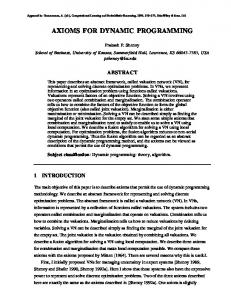
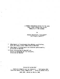
With the estimated and assigned parameter values can we solve the dynamic problem using Policy Iteration Method.13 For the purpose of examining how weather derivatives can affect abatement equipment decisions, we study the dynamic optimization problem under two scenarios: (i) using abatement equipment alone; and (ii) simultaneously using abatement equipment and weather derivatives. In this subsection, basis risk and transaction costs are not investigated, and therefore weather data used here are merely from Summit County, Ohio. The optimal initial abatement investment levels, η ∗ , for scenarios (i) and (ii) are found by examining the dynamic optimization solutions corresponding to a series of different investment levels and picking up the levels with maximum Bellman values. The optimal levels are $105.6 and $67.2 for the two scenarios, respectively. Hence, using weather derivatives can mitigate the problem of high initial installation cost of abatement equipment. Table 2 gives the optimal abatement equipment maintenance/replacement decisions, i∗t , corresponding to all possible states. It can be seen that the decisions for the cases with and without using weather derivatives are quite similar. The only three different decisions show that scenario (i) is a bit inclined to replace the equipment earlier. However, for an equipment no more than 6-year-old, the best strategy is to have maintenance. Figure 1 (a) and (b) give the optimal abatement equipment replacement rules for scenarios (i) and (ii). Without using weather derivatives, a set of new abatement equipment can be used for 9 years before replaced; while with weather derivatives, it can be used for 10 years. Therefore, using weather derivatives can postpone the replacement of abatement equipment. Figure 2 gives the optimal abatement maintenance policies. Under scenario (i), maintenance services should be given each year except the first and last years during the life of abatement equipment; while under scenario (ii), maintenance will not be given in the 8th year besides 13 CompEcon

Toolbox in Miranda and Fackler (2002) is used to perform policy iteration.

19

the first and last years. Thus, using weather derivatives reduces the frequency of maintenance. The optimal purchase amount of weather derivatives φ∗t under scenario (ii) is displayed in figure 3. As can be seen, a farmer should buy more weather derivatives as his abatement equipment turns older, especially in the 8th and 10th years when no maintenance is given. It means that as the equipment turns old, its effectiveness is declining, and therefore more weather derivatives should be used as compensation. The risk management value of weather derivatives and abatement equipment is investigated using equations (29)-(31). First, as a benchmark, suppose this representative farmer employs neither weather derivatives nor abatement equipment. According to our data and estimated β, the mean and variance of his annual revenue loss due to heat stress are $49.69 and 411.19. By the mean-variance utility model, the annual utility loss of the farmer with risk aversion A of 0.20 is (−49.69 − 12 · 0.2 · 411.19) = −90.81 dollars in certainty equiva∞ t t lent. Thus the long-run utility loss from heat stress is ∑∞ t=0 δ Uloss = ∑t=0 0.9 ·90.81 = 908.1

dollars. Under scenario (i), by using abatement equipment alone, the maximized increased t utility in the dynamic optimization, i.e. max ∑∞ t=0 δ ∆Ut , is $248.4 in certainty equivalent. So η,it

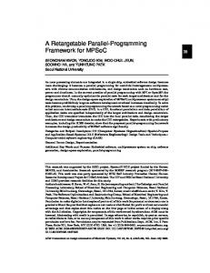
the optimal use of abatement equipment can reduce the utility loss by 27.35%. And under t scenario (ii), the maximized increased utility, i.e. max ∑∞ t=0 δ ∆Ut , is $499.8 in certainty η,it ,φt

equivalent. The optimal use of these two instruments can reduce utility loss by 55.04%. Therefore, using weather derivatives together with abatement equipment can significantly enhance the risk management effectiveness over using abatement equipment alone.

Effect of Basis Risk and Transaction Costs

In this subsection, Cleveland serves as the weather option reference city. Therefore, weather data of Cleveland are used to calculate the payoff and premium of weather options in equations (26) and (27). The option strike level, Ithreshold in (26), is assumed to be chosen by the buyers. The optimal strike levels and optimal initial abatement investment levels are 20

determined by examining the dynamic optimization solutions corresponding to a series of combinations of different strike levels and initial investment levels and then picking up the combinations with highest Bellmans values. And transaction cost loading rate γ is set as 5%. Besides the two scenarios in the last subsection, another two scenarios are analyzed here: (iii) simultaneously using abatement equipment and weather options, but in the presence of geographical basis risk and transaction costs; and (iv) simultaneously using abatement equipment and weather options, but in the presence of both kinds of basis risk and transaction costs. Under scenario (iii), the optimal strike level is 75 degrees of THI, and the optimal initial abatement investment level is $74. The maximized increased utility is $425.4 in certainty equivalent. Under scenario (iv), the optimal strike level is 81 Fahrenheit degrees of temperature, and the optimal initial abatement investment level is $77. The maximized increased utility is $391.3 in certainty equivalent. So although basis risk and transaction costs reduce the risk management effectiveness of weather derivatives, compared with using abatement equipment alone, it still is a significant improvement to use weather derivatives together with abatement equipment in dairy profit risk management (figure 4). The optimal maintenance/replacement decisions under scenarios (iii) and (iv) are the same as those of using abatement equipment alone, i.e. scenario (i). And the optimal weather option purchase amount is displayed in figure 3. Presence of basis risk and transaction costs lowers the optimal purchase amount of weather options.

Conclusion and Discussion In this study, we employ a dynamic programming framework to study the case that a representative dairy farmer maximizes his long-run utility using weather derivatives and abatement equipment to reduce profit loss and risk from heat stress. An exact solution as the optimal

21

risk management strategy for weather derivatives purchase and abatement equipment replacement is derived numerically using policy iteration method. The empirical results suggest that simultaneously using weather derivatives and abatement technologies will outperform using abatement technologies alone, even in the presence of basis risk and transaction costs. And using weather derivatives reduces the investment in abatement equipment, which mitigates the problem of high initial installation cost of abatement equipment faced by small- and medium-size firms. Besides, the optimal purchase of weather derivatives depends on age and maintenance status of abatement equipment. This study introduces a new application of weather derivatives while also exploring the possibilities for hedging a heretofore unhedgable risk. This study yields an analytical solution for a dynamic programming model, which, we believe, provides an applicable guide for the dairy producers. In addition, this research raises many questions of relevance to the economic community, such as the optimal contract design, whether the existence of these contracts reinforces economies of scale in dairy production, what level of sophistication is required to effectively utilize these tools, and finally, what size of a dairy is required to use weather derivatives. These questions may be of interest for further research.

22

References Barth, C. L. “State-of-the-art for Summer Cooling for Dairy Cows.” 52-61, in Livestock Environment II, Proceedings of the Second International Livestock Environment Symposium, Scheman Center, Iowa State Univeristy, April 20-23, 1982. Burt, O. R. “Decision Rules for the Dynamic Animal Feeding Problem.” American Journal of Agricultural Economics 75 (1993): 190-202. Chavas, J.-P., Kliebenstein, J. and Crenshaw, T. D. “Modeling Dynamic Agricultural Production Response: The Case of Swine Production.” American Journal of Agricultural Economics 67 (1985): 636-646. Johnson, H. D. “Bioclimate Effects on Growth, Reproduction and Milk Production.” p. 35, in Johnson, H. D. (ed.) Bioclimatology and the Adaptation of Livestock. Elsevier, Amsterdam, The Netherlands, 1980. McDonald, R. and Siegel, D. “The Value of Waiting to Invest.” Quarterly Journal of Economics 101 (1986): 707-728. McClelland, J. W., Wetzstein, M. E. and Noles, R. K. “Optimal Replacement Policies for Rejuvenated Assets.” American Journal of Agricultural Economics 71 (1989): 147-157. Meyer, J. “Two-Moment Decision Models and Expected Utility.” American Economic Review 77(1987): 421-430. Miranda, M. J. and Schnitkey, G. “An Empirical Model of Asset Replacement In Dairy Production.” Journal of Applied Econometrics 10 (1995): S41-S55. Miranda, M. J. and Fackler, P. Applied Computational Economics and Finance. Cambridge, MA: MIT Press, 2002 National Oceanic and Atomospheric Adiministration, “Livestock Hot Weather Stress.” Reg. Operations Letter C-31-76. US Department of Commerce, National Weather Service, Central Region, Kansas City, Missouri, 1976. 23

Pindyck, R. S. “Irreversibility, Uncertainty, and Investment.” Journal of Economic Literature 29 (1991): 1110-1148. Pratt, J. “Risk Aversion in the Small and in the Large.” Econometrica 32(1964): 122-136. Rust, J. “Optimal Replacement of GMC Bus Engines: An Empirical Model of Harold Zurcher.” Econometrica 55 (1987): 999-1033. Smith, B. J. “Dynamic Programming of the Dairy Cow Replacement Problem.” American Journal of Agricultural Economics 55 (1972): 100-104. St-Pierre, N. R., Cobanov, B. and Schnitkey, G. “Economic Cost of Heat Stress: Economic Losses from Heat Stress by U.S. Livestock Industries.” Journal of Dairy Science 86 (2003): E52-77. Thompson, G. E. “Review of the Progress of Dairy Science Climatic Physiology of Cattle.” Journal of Dairy Research 49(1973): 441-473.

24

Appendix Milk Loss Function The milk loss model in SCS (2003) is: MILK loss = 0.0695 ∗ (THI max − THI threshold )2 ∗ Duration, where MILK loss is in kilogram, and Duration is the proportion of a day where heat stress occurs (i.e. THI max > THI threshold ). The process to calculate the Duration of heat stress:

T HImean = (THI max + THI min )/2 if THI max < THI threshold Duration = 0 elseif THI min >= THI threshold Duration = 24 elseif THI mean > THI threshold threshold −THI mean Duration = (P I − 2 ∗ arcsin( THI THI max −THI mean ))/P I ∗ 12 mean −THI threshold else Duration = (P I + 2 ∗ arcsin( THI THI max −THI mean ))/P I ∗ 12

end

where P I = 3.1415... Abatement Effect Function In SCS, for a 50 m2 cow pen, which can hold 7.1759 dairy cows, when the annualized fixed costs are $310, the corresponding operating costs are $0.0685/hour of operation. And the abatement effect is: ∆THI = −17.6 + (0.36 ∗ T ) + (0.04 ∗ H), where ∆THI is the change in apparent THI, T is ambient temperature (◦ C), and H is ambient relative humidity in percent. Based on the above specifications, we linearly simulate another six abatement effect func-

25

tions corresponding to six fixed cost levels. The six fixed cost levels are 130, 190, 250, 370, 430, 490 dollars respectively. That is, all the parameters in a simulated model are proportional to those in the SCS model, with the proportion equal to the ratio of fixed cost levels. We define the reduced profit loss by: e = max(min(THI max − THI threshold , ∆THI), 0) ∗ β ∗ MILKprice. m

26

Table 1: Summary of Parameters Value Interpretation Equation Estimated Assigned β 0.1617∗∗∗ Sensitivity of profit to weather (6) δ 0.9 Intertemporal discount factor (11) κ 0.8 Abatement effectiveness declining factor (13) n 4 Age’s effect on abatement equipment (13) ∗∗∗ b −32.0920 Abatement effectiveness parameter (13) ∗∗∗ c 0.0029 Abatement effectiveness parameter (13) k1 0.012 Age’s effect on maintenance cost (14) k2 0.02 History’s effect on maintenance cost (14) A 0.2 Pratt’s Absolute Risk Aversion (16)

Symbol

Note: “Equation” in the last column gives the numbers of equations where the parameters show up for the first time. The symbol ∗∗∗ indicates the estimates are at the 1% significance level.

Table 2: Optimal Maintenance/Replacement Decisions Maintenance History

age

1 2 3 4 5 6 7 8 9 10

1 2 2 2 2 2 2 12 1 1 1

2

3

4

5

6

7

8

9

10

2 2 2 2 2 2 2 3 3

2 2 2 2 2 23 3 3

2 2 2 2 3 3 3

2 2 23 3 3 3

2 3 3 3 3

3 3 3 3 3 3 3 3 3

3

Note: Inside the decision matrix, numbers 1, 2, and 3 denote “no action”, “maintenance”, and “replacement” respectively. These numbers are the optimal decisions with using weather derivatives. Numbers in superscripts are different decisions in the case of not using weather derivatives.

27

Optimal Replacement Rule 10

9

9

8

8

7

7

Age of Equipment

Age of Equipment

Optimal Replacement Rule 10

6

5

4

6

5

4

3

3

2

2

1

1

0

1

5

10

15

20

25

0

30

1

5

10

Year

15

20

25

30

Year

(a) Not using weather derivatives

(b) Using weather derivatives

Figure 1: Optimal replacement rule

Optimal Maintenance Rule 10

9

9

8

8

Number of Maintenance Services

Number of Maintenance Services

Optimal Maintenance Rule 10

7

6

5

4

3

2

1

0

7

6

5

4

3

2

1

1

5

10

15

20

25

0

30

1

5

10

Year

15

20

25

Year

(a) Not using weather derivatives

(b) Using weather derivatives

Figure 2: Optimal maintenance rule

28

30

Optimal Weather Derivatives Purchase 100 scenario (ii) scenario (iii) scenario (iv)

90

80

Purchase ($)

70

60

50

40

30

20

10

0

1

5

10

15

20

25

30

Year

Figure 3: Optimal weather derivatives purchase

100 90

Reduction in Utility Loss (%)

80 70 55.04

60

46.85

50

43.09 40 30 27.35 20 10 0 scenario (ii)

scenario (iii)

scenario (iv)

scenario (i)

Figure 4: Comparison of risk management effectiveness

29