A Dynamic Test Cluster Sampling Strategy by Leveraging Execution Spectra Information Shali Yan 1,2, Zhenyu Chen1,2, Zhihong Zhao1,2,*, Chen Zhang1,2, Yuming Zhou1 1
State Key Laboratory for Novel Software Technology, Nanjing University, Nanjing 210093, China 2
Software Institute, Nanjing University, Nanjing 210093, China *corresponding author:
[email protected]
Abstract—Cluster filtering is a kind of test selection technique, which saves human efforts for result inspection by reducing test size and finding maximum failures. Cluster sampling strategies play a key role in the cluster filtering technique. A good sampling strategy can greatly improve the failure detection capability. In this paper, we propose a new cluster sampling strategy called execution-spectra-based sampling (ESBS). Different from the existing sampling strategies, ESBS iteratively selects test cases from each cluster. In each iteration process, ESBS selects the test case that has the maximum suspiciousness to be a failed test. For each test, its suspiciousness is computed based on the execution spectra information of previous passed and failed test cases selected from the same cluster. The new sampling strategy ESBS is evaluated experimentally and the results show that it is more effective than the existing sampling strategies in most cases. Keywords-test selection; cluster filtering; cluster sampling; execution spectra;
I.
INTRODUCTION
Although software testing is essential for ensuring software quality, it is expensive and time-consuming. To reduce testing cost, many automation tools have been developed to generate test inputs, execute programs, and check test outputs. However, in many cases, a formal test oracle specification is not available and test outputs hence have to be checked manually. So, a lot of human efforts are needed if there is a large set of test cases without test oracles. In such a situation, test selection helps to save cost by reducing test size but finding maximum failures. Previous empirical studies have shown that failures caused by the same bug often have similar behaviors [1]. This motivates some researchers to use cluster techniques for test selection, called cluster filtering [2, 3]. Cluster filtering techniques first group test cases with similar execution profiles into the same cluster and then select samples from each cluster [2, 3, 4]. In an ideal situation, if there are m bugs, the failed tests are grouped into m clusters. Each cluster is full of failures caused by the same bug. Therefore, to find these bugs, we only need to randomly *The work described in this article was partially supported by the National Natural Science Foundation of China (90818027, 60803007, 60803008), the National High Technology Research and Development Program of China (863 Program: 2009AA01Z147), the Major State Basic Research Development Program of China (973 Program: 2009CB320703).
select one test from each cluster. This is the one-per-cluster sampling strategy. But in most cases, the result of clustering is not as good as the ideal situation. A cluster is usually mixed with passed and failed tests, or is comprised of failures which are caused by different bugs. On the other hand, it is difficult for programmers to locate bug with only one related failure. More failed tests, even caused by the same bug, are useful for debugging and maintenance. So, we need to find as many failures as possible. The n-percluster sampling is an extension of one-per-cluster sampling, which randomly selects n tests from each cluster. It means to find more failures by selecting more tests. As mentioned in [5], one-per-cluster sampling and n-per-cluster sampling strategies are completely random sampling techniques without any information to guide their selection. An improved technique is adaptive sampling, which first randomly selects one test from each cluster. Then, the outputs of all the tests are inspected and the inspection results (pass or fail) are used to guide the next selections. If a test is failed, then all the other tests in the same cluster are also selected. Previous research shows that adaptive sampling strategy is more effective than n-per-cluster sampling strategy [2]. However, the effectiveness of adaptive sampling strategy largely depends on the inspection result (pass or fail) of the first selected test in each cluster. For a cluster, if the first selected test is a failed test, then all the remaining tests in this cluster are selected even if most of them are passed tests; if the first selected test is a passed test, then all the remaining tests in this cluster are abandoned even if most of them are failed tests. As a result, either only one test or all the tests in each cluster are selected. This may lead to a low efficiency ratio (% failures found) / (% tests sampled). In this paper, we propose a dynamic test cluster sampling strategy called execution-spectra-based sampling (ESBS) 1 . ESBS computes a suspiciousness value for each test case. If the suspiciousness value is larger than a threshold, then the corresponding test is considered to be a possible failed test. Otherwise, it is considered to be a possible passed test. Then, ESBS selects a possible failed test with maximum suspiciousness value from the cluster. After that, ESBS uses the inspection result (i.e. the real pass or fail information) and the execution spectra information of 1 Two terms, profile and spectra, are used in this paper. Profiles are used for tests whose outputs have not been inspected. Spectra are used for tests that have been inspected to be passed or failed.
the selected test to update the suspiciousness values for the remaining tests in the same cluster. This selection process is repeated until there is no possible failed test available in the cluster. The experimental results show that ESBS is more effective than the existing test cluster sampling strategies. This paper makes a number of contributions. First, to the best of our knowledge, it is the first time to use execution spectra information in test selection, although it has been extensively used in fault localization [6, 7, 8, 9]. Second, we propose a dynamic test cluster sampling strategy ESBS by leveraging execution spectra information. Unlike previous cluster sampling strategies, ESBS iteratively selects test cases from each cluster. Third, we conducted an experiment to investigate the effectiveness of ESBS using the commonly used Siemens programs. The experimental results show that ESBS is more effective in finding failures than the existing cluster sampling strategies. The rest of this paper is structured as follows. In section II, we present existing efforts that are related to our work. In section III, we explain our approach and illustrate it with an example. In section IV, we implement the experiments and the experimental results show the effectiveness of ESBS. In section V, we conclude our work and outline the directions for the future work. II.
RELATED WORK
Cluster filtering is a kind of test selection technique, which groups similar execution profiles into the same cluster and then samples from clusters base on a certain strategy [2]. The effectiveness of cluster filtering was evaluated by William et al. [2, 10] and they found that it is more effective than random testing. They also compared the three basic sampling strategies: one-per-cluster sampling, nper-cluster sampling, and adaptive sampling. The results show that, with the same number of tests selected, adaptive sampling can find more failures than one-per-cluster sampling and n-per-cluster sampling [2]. However, with the same cluster count, as n becomes larger, n-per-cluster sampling can find more failures than adaptive sampling, but also more tests are selected. Execution spectra information has been extensively used in fault localization [8, 9]. Hangal and Lam first abstract invariants from the executions of the passed tests. Then, violations of these invariants are abstracted from the executions of the failed tests. These violations are thought to be fault relevant [8]. For each failed test, Manos and Steven find its nearest successful test, and the suspicious parts are the difference between the spectra of two tests [9]. Unlike previous studies, this paper uses execution spectra information to guide test selection. Some researchers have experimentally demonstrated that test reduction and test prioritization can improve the effectiveness of fault localization. Yu et al. [11] compared the effects of different test reduction techniques on faultlocalization. Jiang et al. [12] studied the impact of test prioritization on statistical fault localization. Several test prioritization strategies are compared, and the results show
that coverage-based strategies are the best. This paper introduces the idea of fault localization to test selection. III.
OUR APPROACH
This section presents our execution-spectra-based sampling (ESBS) strategy. We first give a framework to introduce the procedure of ESBS, and then some equations are used to explain our measurement methods. Finally, we use an example to illustrate how ESBS works. A. Framework As shown in Fig. 1, cluster filtering contains three steps: 1) Running tests: all the test cases are executed to get their execution profiles. In this step, function call profile and statement coverage profile are generated for each test. The function call profile gives the number of times each function is called in a run. It was used for cluster analysis. The statement coverage profile gives the set of statements that are executed during a run. It was used to compute the execution spectra for our sampling strategy ESBS. 2) Cluster analysis: the inputs to cluster analysis are the function call profile generated in the first step. Simple K-means clustering algorithm is chosen by us, because it is simple and fast, and moreover, it performs reasonably well in preliminary experiments and gives high quality output. Clustering techniques put tests with similar profiles into the same cluster. Therefore, distances between profiles are calculated. We use Euclidean distance as the dissimilarity metric. If the profiles of two tests are T: and T’: , the distance between them will be: D ( T , T ') =
n ∑ ( t i − t 'i ) 2 i = 1
(1)
The attribute ti represents the number of times the function fi is executed by the test case t. Similarly, the attribute t’i represents the number of times the function fi is executed by the test case t’. 3) Sampling: select tests from each cluster. Our execution-spectra-based sampling (ESBS) strategy is used in this step. The procedure of ESBS is shown in the textbox in Fig. 1. The detailed explanation is as follows. ESBS is a form of adaptive sampling. Each test is selected based on the execution spectra information of the previous selected tests in the same cluster. As shown in Fig.1, ESBS is composed of five phases: • Test selection: select a suspicious test case ti from the cluster whose suspiciousness is the highest. If more than one test case in the cluster has the highest suspiciousness, random selection is applied to decide which one to be selected.
•
Running tests
Execution profiles
•
Cluster analysis • Clusters For Each Cluster Sampling (ESBS) A cluster
Test Selection
A test
•
Result inspection: assign the test case ti to testers for result inspection. The execution spectrum of the passed or failed test case ti will influence the set of suspicious statements and further influence the set of suspicious tests. Statement measurement: re-compute the confidence of each statement based on the execution spectrum of ti. If ti is passed, the confidences of the statements executed by it will be increased; else, the confidences of these statements will be decreased. Statement identification: statements are identified to be correct or suspicious based on their confidence value. We will give a parameter confidenceThreshold (abbreviated as CT). A statement is suspicious if its confidence value is smaller than CT. A statement is correct if its confidence value is equal to or large than CT. Test measurement: computes the suspiciousness of the remained test cases in the cluster. The suspiciousness of a test case is equal to the number of suspicious statements it executes. A test case is suspicious if its suspiciousness is large than 0.
The cycle of the five phases continues, until there is no suspicious test left in the cluster. It means that statements executed by the remained tests are identified to be correct by the execution spectra of the previous selected tests.
Result inspection
Execution spectrum
B. Measurement Methods This subsection explains the measurement methods in ESBS with seven equations.
confidence( s ) = passed ( s ) − failed ( s ) Statement measurement
Confidences of statements
Statement identification
Suspicious statements
Test measurement
Suspicious tests (Suspiciousness) Figure 1. The framework of our approach. The procedure of our execution-spectra-based sampling(ESBS) strategy is shown in the textbox.
(2)
The confidence(s) is a computed confidence value of statement s. The passed(s) represents the number of selected tests that execute statement s and is inspected to be passed. The failed(s) represents the number of selected tests that execute statement s and is inspected to be failed. Intuitively, a statement is more likely to be correct if it is executed by many passed tests and few failed tests. Therefore, for a statement s, ESBS uses the number of passed tests that execute s minus the number of failed tests that execute s as the confidence value of s. Equation (2) is implemented in our algorithm as follows: The confidence of each statement is initialed with 0. After a test is selected, only the confidences of the statements executed by it will be recalculated. If the test is passed, the confidence of each executed statement is increased by 1. If the test is failed, the confidence of each executed statement is decreased by 1. suspicious ( s ) = {s ∈ S | confidence( s ) < CT }
(3)
correct ( s ) = {s ∈ S | confidence( s ) >= CT }
(4)
suspicious ( s ) I correct ( s ) = ∅
(5)
1)
The suspicious(s) is a set of statements whose confidence value--confidence(s) is smaller than CT (the threshold CT is a variable parameter). These statements are considered to be suspicious statements. The correct(s) is a set of statements whose confidence value--confidence(s) is equal to or larger than CT. These statements are considered to be correct statements. There are only two statuses of statements—either suspicious or correct. As shown in equation (5), suspicious(s) and correct(s) are two disjoint sets. After a new test is selected, the confidence value of all the statements executed by it will be recalculated. Therefore, the statuses of these statements may be changed. t ( s ) = {s ∈ S | t executes s}
2)
(6) 3)
suspiciousness (t ) =| t ( s ) I suspicious ( s ) |
(7)
suspicious (t ) = {t ∈ T | suspiciousness (t ) > 0}
(8)
The t(s) is a set of statements that are executed by test case t. The suspiciousness(t) is the suspiciousness of test case t. It equals to the number of suspicious statements executed by t. According to equation (7), the test case that executes most suspicious statements has the highest suspiciousness, and thus it is our next choice. The suspicious(t) is a set of test cases whose suspiciousness is large than 0. In other words, these test cases execute suspicious statements. TABLE II. Order
1 2 3 4
Selected test
t2 t3 t4 t5
Inspection result
pass fail fail pass
At the beginning, the confidences of all the statements are initialized with 0. As CT is 1, all the statements are suspicious. Therefore, t2 is first selected because it executes maximum suspicious statements and thus has the highest suspiciousness 5. Since t2 is inspected to be passed, the confidences of s1, s2, s4, s5 and s6 are increased to 1. Now, s3 is the only suspicious statement whose confidence is smaller than CT. The tests that execute s3 are t3 and t5. Therefore, t3 and t5 have the same suspiciousness 1. We randomly select one from them. Suppose t3 is selected. Since t3 is failed, the confidences of s2 and s3 are decreased by 1. Now, the statements s2 and s3 are suspicious. Among the remained tests, t4 and t5 each executes a suspicious statement and thus have the same suspiciousness 1. Suppose t4 is selected at random. As t4 is failed, the confidences of s2 and s5 minus 1. Thus, there are three suspicious statements – s2, s3 and s5.
TABLE I.
SIX TESTS WITH THE STATEMENTS THEY EXECUTE AND THEIR INSPECTION RESULTS.
Test cases t1 t2 t3 t4 t5 t6
Statements executed s1,s4,s6 s1,s2,s4,s5,s6 s2,s3 s2,s5 s1,s3,s4 s1,s6
Pass or fail pass pass fail fail pass pass
THE DETAILED SAMPLING PROCESS OF ESBS ON THE TESTS IN TABLE I.
The confidence of each statement (confidenceThreshold=1) S1
S2
S3
S4
S5
S6
0
0
0
0
0
0
1 1 1 2
1 0 -1 -1
0 -1 -1 0
1 1 1 2
1 1 0 0
1 1 1 1
C. An Example In this subsection, we give an example to illustrate how ESBS works. As shown in TABLE I, we need to sample from a cluster that contains six tests in column 1. The statements executed by them are in column 2, and their inspection results (pass or fail) are listed in column 3. There are totally six statements (s1 to s6) that are executed by these tests. The bug is in s2, which is executed by one passed test case (t2) and two failed test cases (t3 and t4). In TABLE II, we present how the five phases of ESBS (test selection, result inspection, statement measurement, statement identification and test measurement) run on the tests in TABLE I. In this example, we set CT to 1, which means a statement is not suspicious if its confidence is equal to or larger than 1. The sampling process of ESBS in TABLE II is explained as follows:
4)
5)
Suspicious statements
Remained tests
Suspicious tests (suspiciousness)
s1,s2,s3, s4,s5,s6 s3 s2,s3 s2,s3,s5 s2,s3,s5
t1,t2,t3, t4,t5,t6 t1,t3,t4,t5,t6 t1,t4,t5,t6 t1,t5,t6 t1,t6
t1(3), t2(5), t3(2), t4(2), t5(3), t6(2) t3(1), t5(1) t4(1), t5(1) t5(1) ---
The test cases left are t1, t5 and t6. Only t5 executes a suspicious statement s3. So, t5 is selected because it is the only suspicious test case. As t5 is passed, the confidences of s1, s3 and s4 are increased by 1. Now, the suspicious statements are still s2, s3 and s5. The remained test cases are t1 and t6. Since none of them execute suspicious statements-s2, s3 and s5, they are not suspicious tests. The sampling process stops because there is no suspicious test left in the cluster. At last, suspicious statements (s2, s3, s5) and their confidence value are outputted to help programmers locate bugs. And the same sampling procedure is applied to another cluster.
IV.
EXPERIMENTAL RESULTS
We have performed experiments to evaluate the fault detection efficiency of ESBS and the other sampling strategies. The experimental results are to answer the following questions: • Is ESBS better than the other sampling strategies? • How do the threshold confidenceThreshold(CT) and the cluster count affect the efficiency of ESBS?
C. 1)
2)
A. Subject Programs We experimented with five of the seven classic Siemens programs and their test suits [13]. The detailed information of them is in TABLE III. TABLE III. Program name print_tokens print_tokens2 schedule schedule2 replace
DETAILED INFORMATION OF THE FIVE SUBJECT PROGRAMS
Number of functions 18 19 18 16 21
Line of Code 726 570 412 374 564
Test suite size 4130 4115 2650 2710 5542
The five programs have 16-21 functions and 374-726 lines. There are large test suites that come with these programs. The five programs are small, but have most of the features of c programs—point, memory allocation, different kinds of arithmetic, complex flow control and so on. We only use five of the seven Siemens programs, because the other two programs tcas and totinfo only have 7-9 functions. They are not suitable to calculate the function call profiles for cluster analysis. B. Evaluation Model To evaluate ESBS and other exiting strategies, we use two models, one for calculating the fault detection capability, one for calculating the test reduction capability [2, 10]. 1)
Failure-detection-ratio
3)
4)
Experimental Steps Identify failures: To evaluate the fault detection efficiency of each sampling strategy, we need to know at first who are the failed tests. We compared the test outputs of the correct version with that of the incorrect version. A test is a failure if the two outputs are different. Generate execution profiles: We used gcov (a GNU tool) to record detailed coverage information while execution. Then, we analyzed the information to generate function call profiles and statement coverage profiles for each test. The function call profile gives the number of times a function is called when running a test. It was used for cluster analysis. The statement coverage profile records the line number of statements covered during a run. It was used by ESBS to do cluster sampling. The execution spectrum in Fig. 1 is just the statement coverage profile of the inspected test. Cluster analysis: We used the data mining tool Weka [16] to cluster function call profiles. The clustering technique we chose was K-means with Euclidean distance as the dissimilarity metric. The cluster count were 0.5%, 1%, 5%, 10%, 15%, 20%, 25% and 30% of the test size. Sampling: We wrote programs to implement ESBS and the other sampling strategies. Researchers have found that adaptive sampling is more efficient than one-per-cluster sampling, and n-per-cluster sampling can find more failures when cluster count is fixed [2, 10, 15]. In this paper, we compare ESBS with 3-percluster sampling, and adaptive sampling. All the three sampling strategies have a random step. 3-per-cluster sampling completely selects test cases randomly from each cluster. The first step of adaptive sampling selects a test case at random from each cluster. When several suspicious test cases have the same highest suspiciousness, ESBS also randomly selects one from them. Therefore, for each sampling strategy, we ran them 20 times to get average failure-detection-ratio and test-selection-ratio.
Failure-detection-ratio is used to indicate the fault detection capability. If there are totally M1 failures, and a technique finds M2 of them, then the failure-detection-ratio is calculated as follows: Failure-detection-ratio (% failures found) = M2/M1*100%. 2)
Test-selection-ratio
Test-selection-ratio is used to indicate the test reduction capability. The fewer tests selected, the more human effort saved. If there are N1 test cases, and a technique selects N2 of them, then the test-selection-ratio is as follows: Test-selection-ratio (% tests selected) = N2/N1*100%. Figure2. (a)
Figure2. (b)
Figure2. (d)
Figure2. (c)
Figure2. (e)
Figure2. Comparison between sampling strategies for the five subject programs. Average failure-dection-ratio and test-selection-ratio of 3-per-cluster sampling and adaptive sampling and execution-spectra-based sampling(ESBS) are shown. CT is the abbreviation for confidenceThreshold.
D. Experimental Result In Fig. 2, ESBS is compared with adaptive sampling and 3-per-clsuter sampling. We calculated the failure-detectionratio (% failures found) and test-selection-ratio (% tests selected) of each strategy on the five subject programs. Each line is formed by eight points, which represent eight cluster counts: 0.5%, 1%, 5%, 10%, 15%, 20%, 25%, and 30% of the original test size. As the three sampling strategies have used random selection in some place, the ratios are not stable. Therefore, for each fixed cluster count, we ran each strategy 20 times. Average failure-detection-ratio and testselection-ratio are shown in Fig. 2. The results in Fig. 2 show that, in most cases, our method is more effective. Especially for printtokens, with CT set to 3, ESBS finds 100% of the failures when only
6.95% of the tests are sampled. This is an extremely good performance. Only for schedule, the result of ESBS is not as good as adaptive-sampling, but is not worse than the 3-PerCluster sampling. From Fig. 2, we can also see that, for a certain cluster count, larger CT increases both the number of failures found and the number of tests sampled. For a certain CT, the more clusters, the more tests selected and generally the more failures found. To deeply study the relationship between CT, cluster count and the effectiveness of ESBS, we experimented on schedule2 and printtokens2. The percent of failures found and tests selected for printtokens2 and schedule2 are shown in TABLE IV and TABLE V. We choose 1%, 5% and 20% of the test size as cluster count and use 1, 2, 3, 4, 5, and 6 as CT.
TABLE IV. THE AVERAGE PERCENT OF FAILURES FOUND AND TESTS SELECTED FOR PRINTTOKENS2 WITH VARIOUS CLUSTER COUNT AND CONFIDENCETHRESHOLD(CT). Printtoken2
%cluster=1%
%cluster=5%
%cluster=20%
CT
% failures found
% tests selected
% failures found
% tests selected
% failures found
% tests selected
1
51.44
12.45
72.35
28.39
90.35
52.04
2
79.0
19.64
83.42
42.38
98.17
69.35
3
82.98
23.21
93.69
52.59
99.85
77.46
4
85.83
26.1
97.66
60.16
100.0
81.49
5
86.42
30.46
97.75
65.58
100.0
84.24
6
88.67
36.22
99.17
70.01
100.0
86.32
TABLE V. THE AVERAGE PERCENT OF FAILURES FOUND AND TESTS SELECTED FOR SCHEDULE2 WITH VARIOUS CLUSTER COUNT AND CONFIDENCETHRESHOLD(CT). Schedule2
%cluster=1%
%cluster=5%
%cluster=20%
CT
% failures found
% tests selected
% failures found
% tests selected
% failures found
% tests selected
1
27
3.23
51.77
14.14
82.54
35.85
2
45.54
6.62
83.08
24.66
91.08
57.7
3
54.39
9.04
89.15
32.83
95.07
72.02
4
67.38
12.36
92.93
40.11
96.92
81.32
5
77.23
14.93
93.54
46.77
96.92
87.25
6
78.77
16.97
94.77
53.11
100.0
91.11
The results show that, when the cluster count is small, ESBS can find more failures by increasing CT. In TABLE V, with %cluster=1%, only 27% of the failures are found when CT=1 and 78.77% of the failures are found when CT=6. On the contrary, when cluster count is large, ESBS can find most failures with small CT. As shown in TABLE IV, with %cluster=20%, 90.35% of the failures are found when CT =1 and 100% of the failures are found when CT =4. Then, the increased CT only increases the number of tests selected. Therefore, we can conclude that, to achieve a good performance, small cluster count should be with large CT and large cluster count should be with small CT. The future work is to study with more programs, and give a suggesting CT when cluster count is fixed, or give a perfect match of cluster count and CT. E. Threats to validity The first threat to validity is that we experiment with small c programs, which have only 16-21 functions and 374-726 lines. In practice, the programs are much larger. However, we believe that the five Siemens programs are representative of real programs since they have been studied in many researches. And they have most of the features of c programs—point, memory allocation, different kinds of arithmetic, complex flow control and so on.
Another threat is that the types of errors are limited in the subject programs. We may encounter more different bugs in commercial programs. But the bugs in the Siemens programs are all real-life examples that are generated by the programmers in their programming. The last threat comes from our tools, which generate execution spectra, cluster spectra, and implement sampling strategies. To minimize the threat, we use gcov to record coverage information and rely on the data mining tool Weka [14] to cluster spectra. All the other tools are written by us. But we’ve tested them carefully before our experiments. V.
CONCLUSIONS AND FUTURE WORK
This paper uses the execution spectra information of the previous selected test cases to guide test selection in cluster filtering. Our experimental results show that ESBS is better in failure detection than existing sampling strategies in most case. Nonetheless, there is a great room for improvement. For example, to calculate the confidence of each statement, we use the number of successful tests minus the number of failed tests. This measurement method is simple but may be not effective enough. Indeed, we can learn from more statement suspicious/confidence metrics to improve our method. In this paper, we use the same threshold CT for all the clusters. In the future work, we will investigate whether
it is better to give each cluster or even each statement a special CT. In particular, in order to identify the effects of different bugs on ESBS, we will employ mutation analysis to generate more faulty variants of programs [16]. In addition, we will use more programs to study the effectiveness of ESBS. REFERENCES [1]
[2]
[3]
[4] [5]
[6]
[7]
[8]
[9]
[10]
[11]
[12]
[13] [14] [15]
[16]
Ammann, P. E., and Knight, J. C. Data diversity: An Approach to Software Fault Tolerance. IEEE Trans. Comput., 1998, 37(4): 418– 425. William Dickinson , David Leon , Andy Podgurski, Finding failures by cluster analysis of execution profiles, Proceedings of the 23rd International Conference on Software Engineering, p.339-348, May 12-19, 2001, Toronto, Ontario, Canada Podgurski, A., Masri, W., McCleese, Y., Wolff, F.G., and Yang, C. Estimation of software reliability by stratified sampling. ACM Transactions on Software Engineering and Methodology 8, 9 (July, 1999), 263-283. ANDERBERG, M. R. 1973. Cluster Analysis for Applications. Academic Press, Inc., New York,NY. T. Chen, H. Leung, and I. Mak. Adaptive random testing. In M. J. Maher, editor, Advances in Computer Science - ASIAN 2004: Higher-Level Decision Making. 9th Asian Computing Science Conference. Proceedings. Springer-Verlag GmbH, 2004. J. A. Jones, M. J. Harrold, and J. Stasko. Visualization of test information to assist fault localization. In proceedings of the 24th International Conference on Software Engineering(ICSE’01), pages 467–477, May 2001. H. Agrawal, J. Horgan, S. London, and W. Wong. Fault localization using execution slices and dataflow tests. In Proceedings of IEEE Software Reliability Engineering, pages143–151, 1995. S. Hangal and M.S. Lam, “Tracking down Software Bugs Using Automatic Anomaly Detection,” In Proceedings of the 24th International Conference on Software Engineering,May 2002, pp. 291-301. M. Renieris and S. Reiss. Fault localization with nearest neighbor queries. In Proceedings of the International Conference on Automated Software Engineering, pages 30--39, Montreal, Quebec, October 2003. William Dickinson , David Leon , Andy Podgurski, Pursuing failure: the distribution of program failures in a profile space, Proceedings of the 8th European software engineering conference held jointly with 9th ACM SIGSOFT international symposium on Foundations of software engineering, September 10-14, 2001, Vienna, Austria Y. Yu, J. A. Jones, and M. J. Harrold. An empirical study of the effects of test-suite reduction on fault localization. In Proceedings of the 30th International Conference on Software Engineering (ICSE 2008), pages 201–210. ACM Press, New York, NY, 2008. B. Jiang, Z. Zhang, T.H. Tse, T.Y. Chen, How well do test case prioritization techniques support statistical fault localization, in: Proceedings of the 33rd Annual International Computer Software and Applications Conference (COMPSAC 2009), IEEE Computer Society Press, Los Alamitos, CA, 2009. Software-artifact Infrastructure Repository. http://sir.unl.edu The Weka Home Page. http://www.cs.waikato.ac.nz/ml/weka/, The University of Waikato. David Leon , Andy Podgurski, A Comparison of Coverage-Based and Distribution-Based Techniques for Filtering and Prioritizing Test Cases, Proceedings of the 14th International Symposium on Software Reliability Engineering, p.442, November 17-21, 2003 Ji, C. B., Chen, Z. Y., Xu, B. W., and Zhao, Z. H. A Novel Method of Mutation Clustering Based on Domain Analysis. In Proc. of the 21st International Conference on Software Engineering & Knowledge Engineering (SEKE ’09), 2009, 422-425.