Proceedings of the 46th IEEE Conference on Decision and Control New Orleans, LA, USA, Dec. 12-14, 2007
WePI22.16
A Dynamical System That Computes Eigenvalues and Diagonalizes Matrices with a Real Spectrum Christian Ebenbauer Abstract— The present paper deals with the problem of diagonalizing matrices using a control system of the form A˙ = [U, A], where [U, A] = U A − AU and A, U are real matrices. It is shown that the feedback U = [N, A + AT ] + ρ[AT , A], N diagonal, ρ > 0 allows to solve the diagonalization problem under the assumption that the to be diagonalized matrix has real spectrum. Moreover, in the case of a complex spectrum, the feedback allows to check if a matrix is stable or to compute all eigenvalues of a matrix or roots of a polynomial.
I. INTRODUCTION The understanding of the computational power of dynamical systems and feedback is becoming increasingly important in many different research areas. Over the last decades, increasing attention has been paid, in areas like neuroscience, numerical mathematics, or cell biology, to systems which carry out computations in ways different from those based on digital logic (cf. e.g. [22], [16], [1], [3], [20], [13]). In this paper, control systems of the form A˙ = [U, A], where [U, A] = U A − AU represents the Lie bracket (commutator) and U, A are real matrices, are utilized in order to solve a certain computational problem in a nondigital (analog) fashion, namely the problem of diagonalizing matrices. Systems of the form A˙ = [U, A] are often called Lax systems. This class of systems has very interesting properties and appears in many areas of engineering and science, especially in mathematics, physics, and in control theory. Cf. for example [3] [2] and references therein. The present work is closely related to Brockett’s well-known work [7], see also [4],[6],[5],[10] (a more complete list of references can be found in [16]). In [7] the socalled double bracket flow A˙ = [[N, A], A], where A is a symmetric matrix, N is diagonal, and U = [N, A], has been introduced. This system has many remarkable properties. For example, one property is that the system allows to diagonalize real symmetric matrices in the following sense: if the initial condition is a symmetric matrix A(0) = A0 , then A(t) converges to a diagonal matrix while preserving the spectrum of A0 . Over the last four decades, many systems have been derived in a way similar to that of [7] with many interesting properties. For example, well known are the Toda lattice, Oja’s flow, or the QR flow. A collection of such systems and their properties can be found for example in the book by Helmke and Moore [16] as well as in the references therein. Related to the present results is also [17], where the non-symmetric case is considered. However, in contrast The author is with the Laboratory for Information and Decision Systems, Massachusetts Institute of Technology, USA,
[email protected]. The author is financially supported by the FWF, Austria.
1-4244-1498-9/07/$25.00 ©2007 IEEE.
to the present paper, [17] does not guarantee existence and convergence of the solutions. In this paper, the goal is to find a feedback U = U (A) such that the control system A˙ = [U, A] can be utilized not only to diagonalize symmetric matrices but also nonsymmetric matrices with a real spectrum. The main result of this paper shows that such a feedback indeed exists. It has the form U = [N, A + AT ] + ρ[AT , A] and allows to diagonalize non-symmetric diagonalizable matrices, while preserving the spectrum. From the form of the feedback, it can be seen that the resulting new Lax system is a natural generalization of the double bracket flow. Moreover, for the case of a complex spectrum, it is shown that the derived systems can be used to the check if a matrix is stable or to compute, in an analog (continuous) fashion, eigenvalues of matrices or roots of polynomials. The remainder of the paper is organized as follows: In Section II, the diagonalizing feedback and its properties (Theorem 1, 2, 3) is derived. In Section III, the main results are illustrated on various applications and a conclusion as well as an outlook is given in Section IV. Notations. The transpose of a real n×n matrix A ∈ Rn×n is denoted by AT . The trace of a square matrix A is denoted by trace(A) and the Frobenius norm of A is denoted by kAkF , i.e., kAk2F = trace(AT A). The conjugate of a complex n × n matrix A ∈ Cn×n is denoted by A and the conjugate transposed by A∗ . Moreover, ℜ{A} and ℑ{A} denotes the real, respectively, imaginary part of A and [U, A] = U A − AU denotes the Lie bracket (commutator) with A, U square matrices. II. MAIN RESULTS Consider the control system A˙ = [U, A],
(1)
where A ∈ Rn×n and U ∈ Rn×n are arbitrary real n × n matrices. Then the isospectral property of (1) is a well-known fact, cf. e.g. [2], [11], [23]. For reasons of completeness, a proof is given under the additional assumption that the eigenvalues are pairwise distinct. Lemma 1: Suppose that a given initial condition A(0) of (1) has pairwise distinct eigenvalues, then (1) defines an isospectral flow. Proof: Let q(0), p(0) be the normalized (q(0)∗ p(0) = 1) left and right eigenvector of an eigenvalue λ(0) of A(0). Then it is known [18] (Thm. 6.3.12) that if the eigenvalue
1704
46th IEEE CDC, New Orleans, USA, Dec. 12-14, 2007 has simple multiplicity, it changes according to: ˙ ˙ λ(0) = q(0)∗ A(0)p(0).
(2)
Therefore, one gets: ˙ λ(0) = q(0)∗ [U (0), A(0)]p(0) = q(0)∗ (U (0)A(0) − A(0)U (0))p(0) ∗
(3)
∗
= λ(0)(q(0) U (0)p(0) − q(0) U (0)p(0)) = 0. Hence the derivative of the eigenvalue λ(t) at t = 0 is zero. This implies that the spectrum is preserved under the flow (1), because (3) is valid for each t ∈ (0, Tmax ), where Tmax is the maximal interval of existence of (1). Notice, however, that the left- and right eigenvectors are not preserved, but the existence of the left- and right eigenvectors is guaranteed by the fact that A(t) has the same pairwise distinct eigenvalues as A(0). The isospectral property of (1) is essential for the main results of this paper. The first result below shows that there exists a feedback U which allows to diagonalize nonsymmetric matrices with real spectrum in the following (computational [22]) sense: if the initial condition (=input) A(0) = A0 of (1) is a non-symmetric matrix with real distinct eigenvalues, then the flow (=process of computation) of (1) under a the feedback U = [N, A + AT ] + ρ[AT , A] converges to a diagonal matrix with the eigenvalues as diagonals (=output).
Theorem 1: Suppose that a given matrix A0 ∈ Rn×n has pairwise distinct real eigenvalues λi , i.e., A0 can be written as A0 = T −1 ΛT with Λ = diag(λ1 . . . λn ), λi ∈ R, T ∈ Rn×n , T invertible. Then the solution A = A(t) of (1) with the initial condition A(0) = A0 and with the feedback U = [N, A + AT ] + ρ[AT , A]
lim A(t) = Λπ ,
(“Normalization”) In a first step, it is shown that the derivative of the positive semidefinite function 1 V (A) = trace((A − AT )T (A − AT )) 4 (6) 1 = − trace((A − AT )2 ) 4 is monotonically decreasing along the flow (1) with the initial condition A(0) = A0 and with the feedback (4) for all matrices A with [AT , A] 6= 0. Differentiating (6) with respect to (1) and using the facts trace(AB) = trace(BA) and trace(AT ) = trace(A), one obtains: 1 d V (A) = − trace((A − AT )([U, A] − [AT , U T ])) dt 2 1 = − trace((AT A − AAT )(U + U T )) 2 1 (7) = − trace([AT , A](U + U T )) 2 = − trace([AT , A]U ) = − trace([AT , A][N, A + AT ]) − ρtrace([AT , A]2 ). Now it is important to observe that trace([AT , A][N, A + AT ]) = 0.
(5)
where (π(1), . . . , π(n)) is a permutation of (1, . . . , n), ρ is an arbitrary positive constant, and N ∈ Rn×n is a real, diagonal matrix with pairwise distinct diagonals, i.e., N = diag(n1 . . . nn ), ni 6= nj for i 6= j. Proof: The idea of the proof goes, roughly speaking, as follows. “Normalization” step: First is it shown that the solution A(t) defined by (1), (4), A(0) = A0 , satisfy [A(t)T , A(t)] → 0 for t → ∞, which means A(t) converges to the set of normal matrices, that is the set of matrices which satisfy AT A = AAT , or equivalently A = Θ∗ ΛΘ, Θ∗ Θ = I 1 . Since the spectrum of A(t) is preserved and real, A(t) converges to the compact (bounded) set of symmetric matrices with a fixed spectrum Λ. “Diagonalization” step: Thus, U (t) = [N, A(t)T + A(t)] + ρ[A(t)T , A(t)] ≈ 2[N, A(t)] for t → ∞. From which the diagonalization follows from [7]. 1 Since Λ is real, Θ is also real [18]. However, due to Theorem 2 the conjugate transposed is used instead of the transposed.
(8)
This follows from the fact that the trace of a product between a symmetric matrix ([AT , A]) and a skew-symmetric matrix ([N, A + AT ]) is zero. Thus with trace([AT , A]2 ) = trace([AT , A]T [AT , A]) > 0 one gets d V (A) < 0 ∀[AT , A] 6= 0. (9) dt Therefore, since V is bounded from below, the solution A = A(t) of (1) under the action of feedback (4) converge into the set where the self-commutator vanishes, i.e., lim [A(t)T , A(t)] = 0.
t→∞
(4)
converges to Λπ = diag(λπ(1) . . . λπ(n) ), i.e., t→∞
WePI22.16
(10)
Since the spectrum of A is real, this implies that A converges to a symmetric matrix [18]. Notice that the limit (10) is welldefined, even though the Lyapunov function V is positive semidefinite only. To see this, assume that kA(t)k2F = trace(A(t)T A(t)) → ∞ for t → Tmax , where Tmax is the maximal interval of existence of A(t). On the other hand, it is clear that V stays bounded for t → Tmax , i.e., V (A(t)) ≤ M , M ∈ R. This leads now to a contradiction since Lemma 1 ensures a constant spectrum, i.e., kA(t)k2F → ∞ implies V (A(t)) → ∞ because: 1 V (A(t)) = kA(t)T − A(t)k2F 4 1 = trace(2A(t)T A(t) − A(t)2 − (A(t)T )2 ) (11) 4 1 1 = kA(t)k2F − trace(Λ2 + (Λ∗ )2 ) → ∞. {z } 2 | {z } 4 | →∞
constant
(“Diagonalization”) In a second step, it is shown that the function (compare with [7]) 1 (12) W (A) = trace(N (A + AT )) 2
1705
46th IEEE CDC, New Orleans, USA, Dec. 12-14, 2007 and a solution A(t) of (1), with the initial condition A(0) = A0 under the action of the feedback (4), converges to a matrix A which satisfies [N, A + AT ] = 0. Differentiating (12) with respect to (1) and using the facts trace(AB) = trace(BA), trace(AT ) = trace(A), [A, B] = −[B, A], [A, B]T = [B T , AT ] one obtains2 : d 1 1 W (A) = trace(N [U, A]) + trace(N [AT , U T ]) dt 2 2 1 1 = trace([A, N ]U ) + trace([N, AT ]U T ) 2 2 1 = trace([A, N ]([N, A + AT ] + ρ[AT , A])) 2 1 + trace([N, AT ]([A + AT , N ] + ρ[AT , A])) 2 1 = trace([A, N ][N, A + AT ]) 2 1 + trace([N, AT ][A + AT , N ]) 2 ρ + trace([A, N ][AT , A] + [N, AT ][AT , A]) 2 1 = trace([A + AT , N ][N, A + AT ]) 2 +ρtrace([A, N ][AT , A]). (13) From (10) and (11) follows that any solution A(t) exists for all t > 0 and it converges to the bounded and invariant set Ω = {A : [AT , A] = 0, λ(A) ∈ {λ1 . . . λn }, V (A) ≤ M } defined by normal matrices with a certain (fixed) spectrum. Moreover, it is true that d 1 W (A(t)) = − trace([A(t) + A(t)T , N ]2 ) ≥ 0 (14) dt 2 for solutions A(t) in Ω. Thus, it follows from LaSalle’s invariance principle [15] that solutions A(t) starting in Ω d converge to the set defined by dt W (A(t)) = 0, which implies lim [N, A(t) + A(t)T ] = 0.
t→∞
(15)
Therefore the set {A : [N, A + AT ] = 0} is (conditionally) stable with respect to Ω. Using for example Theorem 3 (Remark 2, Remark 3) from [9] (see also [19]) with V given by (6), (9), it follows that (15) holds for any solution A(t) not necessarily starting in Ω3 . Thus, (10) to together with (15) implies that A(t) converges, since U → 0. Finally, it has to be shown that (15) implies that A(t) → Λπ . To see this, observe that [7], [16] [N, A + AT ] = 0 ⇔ A + AT = 2D
WePI22.16 matrix and since the spectrum of A is real, (10) implies that A converges to a symmetric matrix [18] (p.109, Problem 14). Hence by the isospectral property of (1), the desired result follows: lim A(t) = Λπ .
t→∞
In the following, some remarks concerning Theorem 1 and its relation to [7] are discussed. Remark 1: It is interesting to observe from the proof that the diagonalizing feedback (4) can be decomposed into two components U = Ud + ρUn .
(18)
T
The second component Un = [A , A] plays the role of a “normalizer”. This means, that this component forces A(t) to become normal. The first component Ud = [N, A + AT ] plays the role of a “diagonalizer”. This means, that this component forces A(t) to become diagonal. What is interesting (indeed the main idea) is the fact that the normalization component acts orthogonal to the diagonalization component. This can be seen, for example, in the proof in equation (8). The diagonalizer does not effect the normalization, i.e., the monotonicity of V˙ . In particular Ud ∈ Σ⊥ , Un ∈ Σ,
U ∈ Σ⊥ ⊕ Σ,
(19)
⊥
where Ud takes values in the set Σ of skew-symmetric matrices and Un takes values is the set Σ of symmetric (traceless) matrices. Hence < Ud , Un >= trace(UdT Un ) = 0.
(20)
This orthogonality relation, Un ⊥ Ud , enables the simultaneous (“parallel”) action of both, the normalization and the diagonalization process (see Fig. 1). Finally, the positive constant ρ plays simply the role of a relative gain between Un and Ud . It is easy to see from the proof, that ρ can be even time-varying, i.e., ρ = ρ(t) assuming that, for example, ρ(t) ≥ ρ0 > 0. A0
U
A˙ = [U, A]
A
ρ[AT , A]
(16)
with D diagonal. In particular, ([N, A + AT ])ij = (aij + aji )(nj − ni ) = 0 if and only if aij + aji = 0, i 6= j. Thus, (15) implies that A + AT converges to a real diagonal 2 One can simplify the calculation by using AT ]) = trace([AT , N ][N, A + AT ]).
(17)
[N, A + AT ]
Fig. 1.
the fact trace([A, N ][N, A+
3 Essentially, (15) follows from LaSalle’s invariance principle due to (9) and (14) and the global boundedness of A(t), i.e., a monotonic and bounded sequence (V (A(t)), W (A(t))) must converge (thus V˙ (A(t)) → ˙ (A(t)) → 0). 0, W
Feedback loop for computation.
Remark 2: In contrast to the feedback U = [N, A] used in [7], the feedback (4) is not obtained from a gradient type argument. It is, however, of interest to relate the current results
1706
46th IEEE CDC, New Orleans, USA, Dec. 12-14, 2007 to gradient flows and further investigations are needed. As mention in the introduction, if A is symmetric, then the selfcommutator [AT , A] vanishes in (1) and (4), i.e., the “tripleA” term in A˙ = [[N, A + AT ], A] + ρ[[AT , A], A] disappears and one obtains the double bracket flow A˙ = 2[[N, A], A] [7]. Consequently, the sorting behavior, i.e., the order of the eigenvalues along the diagonals of Λπ is analogous to that of [7]. Confer [7] or [16] for more details. Finally, one can think of (1) and (4) as an (adjoint) flow on the general linear group GL(n, R). Notice that the control U satisfies trace(U ) = 0 and thus takes values in the Lie algebra (indeed in the Cartan decomposition (19) of the semisimple Lie algebra) sl(n, R) = Σ ⊕ Σ⊥ of the special linear group SL(n, R). In the literature, e.g. [8],[16],[2], the Lie group/algebra point of view is the usual way to look at systems like (1). Therefore, further investigations in this direction are interesting, i.e., the interpretation of the current results in the context of sl(n, R), su(n)C = Σ ⊕ iΣ⊥ . What happens in the case of a complex spectrum? To see this, notice that the assumption made on A0 in Theorem 1, i.e., a real spectrum, is not used in the proof of Theorem 1 until the very end. Therefore, the following statements can be made: Theorem 2: Suppose that the eigenvalues of a given matrix A0 ∈ Rn×n have algebraic multiplicity one, where A0 = T −1 ΛT with Λ = diag(λ1 . . . λn ), λi = σi ± iωi ∈ C, T ∈ Cn×n , T invertible. Then the symmetric component A(t) + A(t)T of a solution A = A(t) of (1) with the initial condition A(0) = A0 and with the feedback (4) converges to lim A(t) + A(t)T = 2ℜ{Λπ }.
t→∞
(21)
Proof: From (16) follows that A(∞) = D + S,
(22)
where A(∞) = limt→∞ A(t) and S is a skew-symmetric matrix. Moreover, A(∞) is a normal matrix, i.e., A(∞) = Θ∗ Λπ Θ, Θ∗ Θ = I. Therefore, 2D =A(∞) + A(∞)T = Θ∗ (Λπ + Λ∗π )Θ =2Θ∗ ℜ{Λπ }Θ.
(23)
Thus, the eigenvalues of D are ℜ{Λπ }. Moreover, under the assumption that the eigenvalues of A0 must have pairwise distinct real part, i.e., an eigenvalue configuration like λ1,2 = 3 ± ia, λ3,4 = 3 ± ib, a, b ∈ R, is not allowed, the structure of A(∞) = limt→∞ A(t) can be even more precisely predicted. To see this, observe first: Lemma 2: Suppose A = D + S is a normal matrix, where D = diag(d1 . . . dn ) is diagonal and S = (sij ) is skewsymmetric, then ([A, AT ])ij = ([D, S])ij = sij (dj −di ) = 0, and consequently, if dj 6= di , then sij is zero. Proof: Since A is normal, [A, AT ] = 0. Thus, [A, AT ] = [D + S, D − S] = 2[S, D] = 0.
(24)
WePI22.16 Hence ([D, S])ij = sij (dj −di ) must be zero. Consequently, for example, if d1 6= di , i = 2...n, then si1 = −s1i = 0. Since A(∞) is normal and A(∞) = D + S, D = ℜ{Λπ } (equation (22)), it is indeed possible, due to Lemma 2, to read off the eigenvalues of A0 from A(∞). Theorem 3: Suppose that the eigenvalues of a given matrix A0 ∈ Rn×n have pairwise distinct real part in the following sense: the eigenvalues of A0 have algebraic multiplicity one and there exist no pairwise distinct indices i, j, k such that σi = σj = σk , where A0 = T −1 ΛT with Λ = diag(λ1 . . . λn ), λi = σi ±iωi ∈ C, T ∈ Cn×n , T invertible. Then the solution A = A(t) of (1) with the initial condition A(0) = A0 and with the feedback (4) converges to the form if i = j σπ(i) ±ωπ(i) if σπ(i) = σπ(j) , i 6= j (25) lim (A(t))ij = t→∞ 0 else Proof: From equation (22) follows that A(∞) = D +S and D = diag(d1 . . . dn ) = ℜ{Λπ } = diag(σπ(1) . . . σπ(n) ). Moreover, A(∞) is normal. Thus, Lemma 2 can be applied. Notice that, due to pairwise distinct real parts, there exist no three pairwise distinct indices i, j, k such that di = dj = dk . Case 1 (complex eigenvalue): If (A(∞))ii = limt→∞ (A(t))ii = di = σπ(i) = dj for some i and j(6= i) in {1, ..., n}, then the only element in the ith column/row and jth row/column of S which does not vanish is sij (sji = −sij ). In particular, for all k different from i and from j, Lemma 2 and pairwise distinct real parts imply dj − dk 6= 0 and di − dk 6= 0 and thus skj = 0 and ski = 0 for all k 6= i, j. Case 2 (real eigenvalue): If for some i, di = σπ(i) 6= dk for all k 6= i then by Lemma 2, the ith column/row of S vanishes. By writing down S = (sij ) and by taking into account that the eigenvalues of A0 are identical with the eigenvalues of A(∞), it can be easily observed that the non-vanishing entries in S must be equal to sij = ±ωπ(i) . By relabeling the rows/columns of A(∞) such that σπ(i) , σπ(j) are neighbors, in case σπ(i) = σπ(j) , i 6= j (similarity transformation with permutation matrix), one can easily obtain the canonical form (2.5.9),(2.5.10) on p.105 [18]. Thus, the eigenvalues of A0 can be read off from A(∞). Summarizing, Theorem 3 establishes the following structure of A(∞). If for example dk = σπ(k) is simple (real eigenvalue λπ(k) = σπ(k) ), then the kth column and row of A(∞) is zero except the diagonal element (A(∞))kk = dk = σπ(k) . If for example di = σπ(i) = σπ(j) = dj , i 6= j, (complex eigenvalue λπ(i) = σπ(i) ±iωπ(i) ), then one obtains a structure of the form .. . σπ(i) · · · ±ωπ(i) . . . .. .. .. A(∞) = (26) . ∓ωπ(i) · · · σπ(j) .. .
1707
46th IEEE CDC, New Orleans, USA, Dec. 12-14, 2007 III. APPLICATIONS Simulation Example. The first example shows some numerical simulations for various gains ρ with 3 2 −2 1 (27) A0 = 0 2 0 0 1 and N = diag(1, 2, 3) (see Figure 2). From several simula-
WePI22.16 The eigenvalues of A0 are 1, −2.0980, and −0.9510 ± 3.0175i. Using N = diag(1, 2, 3, 4) and ρ = 1, one obtains for A(4) (see Fig. 3) −2.0980 0.0002 0.0004 0.0000 0.0002 −0.9513 3.0178 0.0000 −0.0004 −3.0177 −0.9507 −0.0000 . (29) −0.0000 −0.0000 −0.0000 1.0000 Since there is a positive diagonal element in A(4), the matrix A0 is not stable.
Diagonals of A(t)
Diagonals of A(t)
3.5
1
3
0.5 0
2.5
−0.5
2
−1 −1.5
1.5
−2
1 0.5 0
−2.5
0.5
1
1.5
−3 0
2
Norm of the off−diagonals of A(t)
0.5
Fig. 3.
3
1 Time
1.5
2
Simulation results for (28).
2.5 2 1.5 1 0.5 0 0
0.5
1 Time
1.5
2
Fig. 2. Simulation results for (27) with ρ = 0.5 (dashdot), ρ = 1 (dashed), and ρ = 2 (solid).
tions it has been observed that the behavior of convergence is sensitive to the initial condition, i.e., the norm of A0 . For future research, time-varying gains ρ = ρ(t), may be useful to improve convergence rates (performance) of the flow. Moreover, although Theorem 1 assumes that A0 has to have pairwise distinct eigenvalues, numerical simulations show convergence also when the algebraic and geometric multiplicity is different, since an arbitrarily small perturbation of the eigenvalues, caused for example by numerical errors, may lead to algebraic multiplicity one. Thus, in numerical simulations, one can expect guaranteed convergence for any initial condition. Application 1. From Theorem 2 follows that the diagonals of A(∞) correspond to the real part of the eigenvalues. Therefore, the system (1), (4) can be used to check if a matrix A0 is stable (Hurwitz) by inspecting the diagonals of A(∞). Consider, for example, the matrix −1 2 1 1 −2 −3 0 2 . (28) A0 = 0 0 1 0 −3 −2 −2 0
Application 2. Finding roots of polynomials has a long history in science. Nowadays, any good scientific software package has a function like “root” to find roots of polynomials. However, before the advent of digital computers, the computation of roots of polynomials was not an easy task and needed considerable effort. The paper [14] entitled “machines for solving algebraic equations” gives a nice overview of the effort to build (electro)mechanical machines for finding roots of a polynomial, where the first machines were already build in the 18th century (see also [21]). With the results in this paper, it is possible to get another “machine” which computes (real and complex) roots of polynomials in an analog fashion. To see this, inspect the result above (matrix (29)). It can be seen that the imaginary parts of the eigenvalues can be read off as well. This is in general not the case, even though it happens (almost) always in simulations. However, it is true under the assumptions made in Theorem 3. Hence, the roots of polynomials can be immediately read off from A(∞), as demonstrated below. Consider for example the polynomial (see Fig. 4) p(x) = x4 − 3x2 + x − 1. Forming the companion matrix 0 1 0 0 A0 = 0 0 1 −1
0 1 0 3
0 0 , 1 0
one obtains for N = diag(1, 2, 3, 4) and ρ = 1 −1.944 0.0006 −0.0002 0.0000 −0.0006 0.1442 0.5382 −0.0005 A(2) = −0.0002 −0.5382 0.1383 0.0014 0.0000 −0.0005 −0.0013 1.6615
1708
(30)
(31)
.
46th IEEE CDC, New Orleans, USA, Dec. 12-14, 2007
WePI22.16
y=p(x)
R EFERENCES
2 1
X: 1.667 Y: 0.05672
X: −1.945 Y: 0.01005
0 −1 −2 −3 −4 −1.5
−1
−0.5
0
0.5
1
1.5
2
x
Fig. 4.
Graph of (30).
From the matrix above, the structure of A(∞), as predicted by Theorem 3, can be clearly seen and the real roots as well as the complex roots can be read off from A(2). Another application is to check definiteness of a polynomial. Consider the polynomial p(x) = x4 − 2x3 + x2 + 3x + 3.
(32)
Again, if A0 is the corresponding companion matrix and N = diag(1, 2, 3, 4) and ρ = 1, then one gets as solution −0.6146 0.5680 −0.0001 0.0000 −0.5676 −0.6166 0.0003 0.0002 . A(2) = 0.0001 0.0003 1.6156 1.2912 −0.0000 −0.0002 −1.2912 1.6156 Since there is no column/row with only a diagonal element in it, it follows that all eigenvalues have an imaginary part and since the polynomial p has even degree, it must be positive definite. Moreover, the complex roots can be read off because Lemma 2/Theorem 3 (d1 = d2 6= d3 = d4 ) implies s13 = s23 = s14 = s24 = 0 (sij = −sji ). IV. CONCLUSION AND OUTLOOK The main result of the present paper is a new Lax system which allows to diagonalize non-symmetric matrices and to compute their eigenvalues. Therefore, the present results extend the results for symmetric matrices [7] in a natural way. Moreover, the results can be helpful for designing new numerical algorithms [12]. The idea behind the new diagonalizing system is to define a feedback with a normalizing and a diagonalizing component such that the diagonalization process does not influence the normalization process. Some applications in the context of utilizing dynamical systems for computational purposes have been pointed out. For example, a stability test for matrices as well as roots computation for polynomials. Several points for future research has been discussed. In particular, the connections, interpretations, and generalizations of the present results in the context of Lie groups and Lie algebra.
[1] P.A. Absil. Continuous-time systems that solve computational problems. International Journal of Unconventional Computing, 2:291–304, 2006. [2] O. Babelon, D. Bernard, and M. Talon. Introduction to Classical Integrable Systems. Cambridge University Press, 2003. [3] M.A. Belabbas. Hamiltonian Systems for Computation. PhD thesis, Harvard University, 2006. [4] A.M. Bloch. Steepest descent, linear programming and Hamiltonian flows. In J.C. Lagarias and M.J. Todd, editors, Mathematical developments arising from linear programming, volume 114, pages 77–88. Contemporary Mathematics, A.M.S., 1990. [5] A.M. Bloch, R.W. Brockett, and T.S. Ratiu. Completely integrable gradient flows. Communications in Mathematical Physics, 147:57– 74, 1992. [6] A.M. Bloch, H. Flaschka, and T.S. Ratiu. A convexity theorem for isospectral manifolds of Jacobi matrices in a compact Lie algebra. Duke Mathematical Journal, 61(1):41–66, 1990. [7] R.W. Brockett. Dynamical systems that sort lists, diagonalize matrices, and solve linear programming problems. Linear Algebra and its Applications, 146:76–91, 1991. [8] R.W. Brockett. Differential geometry and the design of gradient algorithms. Proceedings of Symposia in Pure Mathematics, 54:69– 92, 1993. [9] R. Chabour and B. Kalitine. Semi-definite Lyapunov functions: stability and stabilization. rapport technique, Universite de Metz, 2002, no 2, Prepublication du departement de mathematiques, Available from www.math.univ-metz.fr/∼chabour/Articles/SemiDefinite Lyapunov Funtions Stability and Stabilizability.ps, to appear in IEEE Transactions on Automatic Control. [10] M.T. Chu and K.R. Driessel. The projected gradient method for least squares matrix approximations with spectral constraints. SIAM Journal of Numerical Analysis, 27:1050–1060, 1990. [11] P. Deift, T. Nanda, and C. Tomei. Differential equations for the symmetric eigenvalue problem. SIAM Journal of Numerical Analysis, 20:1–22, 1983. [12] A. Edelman, T.A. Arias, and S.T. Smith. The geometry of algorithms with orthogonality constraints. SIAM Journal of Matrix Analysis Applications, 20:303–353, 1998. [13] P. Fern´andez and R.V. Sol´e. The role of computation in complex regulatory networks. In E. V. Koonin, Y.I. Wolf, and G.P. Karev, editors, Power Laws, Scale-Free Networks and Genome Biology, pages 206–225. Molecular Biology Intelligence Unit, Springer Verlag, 2007. [14] J.S. Frame. Machines for solving algebraic equations. Mathematical Tables and Other Aids to Computation, 1(9):337–353, 1945. [15] W. Hahn. Stability of Motion. Springer Verlag, 1967. [16] U. Helmke and J.B. Moore. Optimization and Dynamical Systems. Springer Verlag, 2nd edition, 1996. [17] G. Hori. Isospectral gradient flows for non-symmetric eigenvalue problem. Japan J. Indust. Appl. Math., 17:27–42, 2000. [18] R. A. Horn and C. R. Johnson. Matrix Analysis. Cambridge University Press, 1985 (Reprint 1999). [19] A. Iggidr, B. Kalitine, and R. Outbib. Semidefinite Lyapunov functions stability and stabilization. Journal Mathematics of Control, Signals, and Systems (MCSS), 9:95–106, 1996. [20] W. Maass, P. Joshi, and E. Sontag. Computational aspects of feedback in neuronal circuits. Computational Biology, 3:e165:1–20, 2007. ¨ [21] P. Riebesell. Uber Gleichungswagen. Zeitschrift f. Math. und Phy., 63:256–274, 1914. [22] H.T. Siegelmann. Neuronal Networks and Analog Computation. Beyond the Turing Limit. Birkh¨auser, 1999. [23] D.S. Watkins and L. Elsner. Self-similar flows. Linear Algebra and its Applications, 100:213–242, 1998.
1709


![A chaotic dynamical system that paints arXiv:1504.02010v1 [nlin.CD] 8 ...](https://m.moam.info/img/260x300/a-chaotic-dynamical-system-that-paints-arxiv150402_5b42043c097c4744428b4597.jpg)