Mar 31, 2002 - to describe the turbo decoding algorithm (TDA) as an elegant discrete dy- ... In section 4, the TDA is modeled as a discrete dynamical system.
A Dynamical System View for the Turbo Decoding Algorithm Based on the Gaussian Approximation Arun Rangarajan ∗ Vinod Sharma March 31, 2002
ABSTRACT The Gaussian approximation has been used to study iterative decoding algorithms of graph-based codes like turbo codes [7, 8] and low-density parity check (LDPC) codes [6]. In this work, the Gaussian approximation is used to describe the turbo decoding algorithm (TDA) as an elegant discrete dynamical system and explicit iterative equations for the evolution of the BER with the decoder phases of the TDA are presented. This formulation is used to study the SNR thresholds for turbo codes and the fixed points of the TDA. The issues of stability of TDA’s fixed points for SNRs below the threshold and rate of convergence of the TDA to very low BERs for SNRs above the threshold are also addressed.
Keywords: Turbo decoding algorithm, dynamical system, phase trajectories, indecisive fixed points
1
Introduction
Turbo codes were introduced in the seminal work of [3]. The iterative decoding algorithm introduced in [3] is a low complexity sub-optimal decoding algorithm for turbo codes, since maximum-likelihood decoding (MLD) for turbo codes is prohibitively complex [3, 2]. Though turbo codes are well understood with MLD, their astonishing performance with iterative decoding is still not fully understood. In [4] it was observed that on an additive white Gaussian noise (AWGN) channel, ∗
His work was supported by the DRDO-IISc program on Mathematical Engineering.
1
the histogram of the extrinsic information in the turbo decoding algorithm (TDA) converges towards a Gaussian law as the number of iterations increases. Motivated by this observation and Wiberg’s suggestion [13], the TDA has been studied using the Gaussian approximation in [7, 8]. In [8], the extrinsic information SNR input/output relation of the constituent decoders (CDs) was obtained through simulations to determine whether the TDA will converge or not at a particular Eb /N0 . To obtain the input/output relation at each intrinsic SNR, only one CD was simulated (assuming symmetry of the turbo code) with Gaussian intrinsic and a priori inputs and the output extrinsic information SNR was measured, assuming it to be Gaussian. In this work, the Gaussian approximation is used to describe the TDA as a discrete dynamical system and explicit iterative equations that describe the evolution of the BER with the decoder phases (half-iterations) of the TDA are derived. In [8] the a posteriori probability (APP) decoder was simulated for each Eb /N0 to study the input/output SNR relation. Such an approach was followed because analytical approaches for the APP decoder are very difficult (also see [12]). In this work, we first present an upper bound on the BER of a Viterbi-type CD (named Apriori-Viterbi Algorithm or in short, Apri-VA) for a given Eb /N0 and a priori SNR. This bound is useful for studying the TDA (using a Viterbi-type CD) only at high a priori SNRs for a given Eb /N0 . Hence we resort to simulations as in [8], but simulations are done for an APP decoder only for a few values of Eb /N0 s and a priori SNRs and an analytical expression for the BER is obtained by means of curve fitting over the simulated BERs using the least squares error (LSE) criterion. This expression for BER is then used to study the TDA as a discrete dynamical system at all Eb /N0 s. Using such a formulation, SNR thresholds and stability of the fixed points of the TDA can be studied elegantly. Once offline simulations are done for a CD and an expression for BER is obtained, a CD is fully characterized in the sense that any combination of this CD with other CDs can be studied. Such an approach greatly simplifies the study of both symmetric and asymmetric turbo codes. The rest of the paper is organized as follows. In section 2 the turbo decoder is briefly explained and the notations are introduced. In section 3 an analytical approach to study the TDA and an upper bound on the BER for a Viterbi-type CD are presented. In section 4, the TDA is modeled as a discrete dynamical system by deriving an iterative equation for the BER with decoder phases. This model is then used to study thresholds for turbo codes, stability of TDA’s fixed points (for SNRs below threshold) and rate of convergence of the TDA to very low BERs (for SNRs above threshold). Section 5 gives the conclusions.
2
2
The Turbo Decoder
In this section, an overview of the turbo decoder is given and the notations are introduced. For our current discussion, assume that the turbo code is symmetric i.e., both the constituent recursive systematic convolutional (RSC) codes used for parallel concatenation are the same (extension to asymmetric turbo codes is straight forward as will be seen). Thus only one CD may be studied to understand a symmetric turbo decoder. The entire turbo coded communication system is shown in Fig. 1. The turbo encoder is made of a parallel concatenation of two RSC codes, whose inputs are connected by a random interleaver INT of size N . The second RSC code has √ part punctured. The bit-to-BPSK signal map is given by 0 7→ √its systematic − Es ; 1 7→ + Es . The turbo decoder consists of two CDs, DEC1 and DEC2, each of which could either be an APP decoder or a soft-output Viterbi algorithm (SOVA) decoder. These CDs typically use the log-likelihood ratios (LLRs), instead of the received signals themselves, and hence the signal-to-LLR converters appear before the CDs in Fig. 1. Since turbo codes are linear (and source and channel symmetry are assumed), for performance analysis, assume that 0c , the all-zero codeword, is transmitted w.l.o.g. In Fig. 1, c represents the transmitted codeword, s represents the transmitted BPSK signal vector, y represents the received vector and each of these vectors is of length 3N . The N -length vectors y(1) , y(2) and y(3) are obtained by de-multiplexing y and they represent the received information vector, first-parity vector and second-parity vector respectively; Z(1) , Z(2) and Z(3) represent their corresponding N -length LLR vectors. In Fig. 2 DEC1 is shown. A represents the a priori LLR vector for the information bits, D represents the APP vector output of the decoder, E represents the extrinsic information vector output by DEC1 and each of these vectors is of length N . E is interleaved to obtain the a priori input for DEC2. From now on, by nth phase, we mean the first phase, if n is odd and the second phase, if n is even of the b(n + 1)/2cth iteration.
3
An Analytical Approach for the TDA
In this section an analytical approach to study the TDA is presented. First we state the Gaussian assumption: LLR vectors A, D and E are assumed to be Gaussian. (Z(1) and Z(2) are anyway Gaussian as will be clear from (2).) Note that the independence assumption made in [8] is not made. The LLR can be expressed in terms of the received signal as follows. Consider the ith (i = 1, 2, 3, . . . , 3N ) component of the multiplexed received vector y (see 3
Fig. 1). Its LLR can be written as P (ci = 1|yi ) P (ci = 0|yi ) √ p(yi |si = + Es ) √ = log p(yi |si = − Es ) √ 2 Es yi , i = 1, 2, . . . , 3N, = σ2
Zi = log
(1) (2)
where σ 2 is the variance of the AWGN. Equation (1) follows from the fact that ci (and hence si ), i = 1, 2, 3, . . . , 3N , are a priori equiprobable due to linearity of turbo code. It is clear that, if yi is√ Gaussian, Zi is Gaussian. Assuming all-zero codeword transmission, yi ∼ N (− E s , σ 2 ), for all i. Hence (j)
Zi
�
∼ N −4
Es Es ,8 , j = 1, 2, 3, i = 1, 2, . . . , N, N0 N0 �
(3)
where N0 = 2σ 2 and Z(j) are the LLR vectors associated with y(j) , j=1,2,3. From (3) it is clear that the SNR associated with the received signal is sufficient to characterize the intrinsic LLR. (This SNR will be called as the SNR associated with the LLR.) A similar statement holds for the other LLRs A,D and E by the Gaussian assumption. (Note that A, D and E do not have any explicit signals associated with them. In [5] these LLRs are assumed to be obtained from a meta channel. Also see [7].) The SNRs associated with A,D and E are represented as SA , SD and SE respectively. Now using the Gaussian assumption, Aj ∼ N (−4SA , 8SA ), Dj ∼ N (−4SD , 8SD ) and Ej ∼ N (−4SE , 8SE ), for j = 1, 2, 3, . . . , N . Suppose for a given Eb /N0 and a priori SNR SA , the bit-error probability at the output of DEC1 is Pb . Observe that using the Gaussian approximation, one can view D as the LLR of an AWGN channel output. Hence SD can be written as SD =
(Q−1 (Pb ))2 , 2
where
(4)
1 Z ∞ −z2 /2 √ Q(x) = e dz. (5) 2π x In [8], (4) was used to compute the extrinsic SNRs, after measuring the BERs associated with the simulated extrinsic LLRs. Extrinsic information E is obtained by subtracting A and Z(1) from D (for DEC1). This is done to make the feedback from a CD independent of its inputs
4
[4]. In other words, E can be assumed independent of A and Z(1) as was assumed in [8]. But notice that (1)
Dj = Aj + Ej + Zj , j = 1, 2, 3, . . . , N,
(6) (1)
and hence the mean of Dj is the sum of the means of Aj , Ej and Zj (whether Aj , (1) Ej and Zj are independent or not). By using the mean values provided above, we can write Es SD = SA + S E + . (7) N0 Thus SE can be computed using Es (Q−1 (Pb ))2 SE = − SA − . 2 N0
(8)
This SE is the a priori SNR for the next CD. The above can be used to study the TDA as follows: S1 For a given Eb /N0 , let the bit-error-probability at the output of DEC1 at the end of the first phase be Pb . (The details for estimating Pb are given in Sec. 4.) S2 SE can be computed using (8) with the Pb computed in the last step. (For the first phase alone SA = 0.) S3 SE computed in the last step is SA for DEC2, since interleaving does not change SNR. Thus SA is obtained for DEC2. S4 Having obtained SA for DEC2, the BER at the output of DEC2 can be computed using the methods which will be explained. S5 Having obtained the BER at the output of DEC2, once again (8) can be used for getting SE for DEC2, which is SA for DEC1 (for the third phase). The above steps can be iterated to study the TDA for any number of iterations. These steps give the basis for viewing the TDA as a discrete dynamical system in Sec. 4. Now the problem of finding Pb , given Eb /N0 and a priori SNR SA is addressed. For an APP CD such an analysis is very difficult [12]. With a SOVA CD an upper bound analysis can be done. In fact, the analysis need not be done for a soft-output decoder, but for a Viterbi algorithm (VA) decoder which can use a priori LLR and produce hard-outputs, since only the bit-error probability at the output of a CD is needed. We call a VA which can use a priori LLR as Apri-VA, following [9]. (See [9] for details of the algorithm.) 5
We followed [10] to derive an upper bound for the BER of an Apri-VA for a given Eb /N0 and SA , in a way similar to the derivation of the usual union bound for VA. The bound is presented here and the reader is referred to [11] for details of the proof. Consider a rate-b/c convolutional encoder of memory m. Let df be the free distance of the convolutional code. The bit-error probability Pb after decoding using Apri-VA can be upper bounded as � �q 1 SA ∂T (W, L, I) Pb < Q 4SA e , E −R b b ∂I N0 ,I=e−SA ,L=1 W =e
(9)
where SA is the SNR associated with the a priori LLR and T (W, L, I) is the Extended Path Enumerator (EPE) of the convolutional code. The bound is now studied for an example RSC code.� In Figs. 3,� 4 and 5, the 1+D2 bound is plotted for the rate- 12 RSC code with G(D) = 1, 1+D+D for Eb /N0 s 2 of 0, 0.5 and 1 dBs. Each of these figures is obtained by fixing Eb /N0 and varying SA . A comparison of the bound with the simulation results shows that the bound is tight at high a priori SNRs and pessimistic at moderate a priori SNRs. Notice that the bound is slack at low a priori SNRs. (The simulation results shown in Figs. 3, 4 and 5, are obtained with an APP decoder. We observed that the BER performance of an Apri-VA is close to that of an APP decoder.) The tightness of this bound is similar to that of the usual union bound with no a priori information. In particular, for a fixed Eb /N0 , the bound becomes tighter, as SA increases and vice-versa. Along with the bound and the simulation results, curve fits for the simulated BERs are also shown, which will be explained in Sec. 4.
4
The TDA as a Discrete Dynamical System
In this section, the steps in Sec. 3 are used to study the TDA as a discrete dynamical system. In Sec. 4.1 the TDA is modeled as a discrete dynamical system. In Sec. 4.2 this model is used to analyze the TDA.
4.1
Modeling the TDA as a Discrete Dynamical System
In this subsection, the TDA is modeled as a discrete dynamical system. Such a model for the TDA is best explained with an example. Consider the rate-(1/3) turbo code, which is � � symmetric and whose constituent 1+D2 RSC codes are given by G(D) = 1, 1+D+D2 . (In octal notation the turbo code is called 5/7 turbo code.) Assume a random interleaver whose size is very large, since the Gaussian assumption is valid only for very large interleaver sizes [7, 8]. 6
Now the steps in Sec. 3 are used to model the TDA as a discrete dynamical system. To start the iterations the BER at the end of the first phase is needed (see S1 of Sec. 3). Since our SNR range of interest is very low (near Shannonlimit), the known bounds are not useful. Nevertheless for SNRs away from the SNR threshold, the exact value of the first phase BER is not important for the convergence study of the TDA. On the other hand, for studying the exact phase trajectories [1] and for analyzing the TDA for SNRs near the threshold, precise initial conditions are required. One can use either a VA or an APP decoder for obtaining the first phase BER, since no a priori information is available for the TDA in first phase. For our study, first phase BER was obtained using simulations of an APP decoder. Having obtained this BER, SE can be computed using (8) (with SA = 0). This SE is the a priori SNR for DEC2 (for the second phase of the TDA). Bound (9) can now be used to upper-bound the BER at the output of DEC2, but the bound is useful only for high a priori SNRs. At the end of the first phase, the a priori SNR is so low that the bound cannot be used for upper bounding the BER. Hence we are forced to use a functional approximation using curve fitting over the simulated BERs, for low and moderate a priori SNRs. Our objective now is to get an expression for the BER at the output of an APP decoder, for a given Eb /N0 and SA . On AWGN channels, the BER falls exponentially with Eb /N0 for any coded system. Also, for a given Eb /N0 , the BER falls exponentially with SA (which is clear from the simulation results and the bound at high SNRs). Hence a good functional approximation for the BER is Pb
�
Eb , SA = exp N0 �
�
α
Eb + βSA + γ , N0 �
(10)
where α, β and γ are curve-fit parameters. Once α, β and γ are found for an RSC code, the BER can be obtained for any Eb /N0 and SA . The LSE criterion is used for obtaining α, β and γ. First Eb /N0 is fixed at some value of interest. Then a priori SNR is varied over some range and simulations are done for estimating the BER at each a priori SNR. Next Eb /N0 is changed to some other value of interest and the simulations are repeated by varying the a priori SNR. Simulations for two different Eb /N0 values of 0 dB and 1 dB and SA values from –12 dB to 3 dB, in steps of 1 dB, give good estimates of α, β and γ. (The lower limit for SA is chosen based on the BER at the end of the first phase for an Eb /N0 of 0 dB and the upper limit is chosen based on the closeness of the bound to simulations.) The values of α, β and γ for the 5/7 turbo code were found to be –1.7579, –2.4647 and 0.02555 respectively. The curve fit is shown in Figs. 3, 4 and 5, along with the simulation results and the upper bound of Sec. 3. Notice from the figures that one can use bound (9) for high a priori SNRs (greater than 3 dB for Eb /N0 s of our interest). Nevertheless the curve-fit itself provides a 7
good enough estimate for BER at high a priori SNRs too and hence the curve fit is used for all SNRs. Now an explicit equation relating the BER at the end of one phase with the BER at the end of the previous phase is derived from (8) and (10). Let δ := α(Eb /N0 ) + γ. Let SEn , SAn and SDn denote the SNRs of the extrinsic LLR, a priori LLR and the APP LLR of the nth phase. The BER at the output of the (n + 1)st phase can be written as Pn+1 = exp(δ + βSAn+1 ) = exp(δ + βSEn ) �
�
= exp δ + β SDn − SAn
Es − N0
��
.
(11)
Now using 2
(Q−1 (Pn )) SDn = (12) 2 as a function of Pn , the following equations can be de-
and (10) for writing SAn rived from (11). Pn+1
� � � � exp β (Q−1 (Pn ))2 exp δ − β Es , n = 1 2 � N0 � = 1 β Es −1 2 exp (Q (P )) + 2δ − β , n≥2 n P 2 N n
(13)
0
The TDA is described as an elegant discrete dynamical system by (13). In [7], CD1 and CD2 were modeled as nonlinear mappings of input SNRs to output SNRs, for a given Eb /N0 . An explicit functional form for the maps Gi , i = 1, 2, of [7] can be derived from (11) as follows: SEn+1 = G(SEn , Eb /N0 ) =
�
�
Q−1 eδ+βSEn 2
��2
− SEn − R
Eb , N0
(14)
for n ≥ 1. (The subscript for G is dropped assuming a symmetric turbo code/decoder.)
4.2
Analysis of the TDA as a discrete dynamical system
In this subsection, the TDA is studied as a discrete dynamical system using (13). In Fig. 6 Pn+1 is shown as a function of Pn (for n ≥ 2), for various Eb /N0 s for the 5/7 turbo code. The TDA goes to zero BER with the number of iterations (asymptotically), only if the input-output BER curve does not intersect the (In = Out) line.
8
An estimate for the SNR threshold can be found from Fig. 6. For an Eb /N0 of 0 dB the curve intersects the (In = Out) line, and hence the threshold is greater than 0 dB, whereas for an Eb /N0 of 0.1 dB the curve does not intersect and hence the threshold is less than 0.1 dB. In Fig. 7, the BER input-output relation (for n ≥ 2) is plotted for an Eb /N0 of –0.2 dB for the 5/7 turbo code. Note that the stable indecisive fixed point [1] corresponds to a BER greater than 0.1. This fixed point attracts all BERs which are greater than the BER value marked ‘Unstable fixed point,’ which corresponds to a BER of nearly 9 x 10⁻³ . (In dynamical system terminology, all the BERs greater than the unstable fixed point are in the basin of attraction of the indecisive fixed point.) Hence if the BER at the end of the second phase of the TDA (P2 ) is less than (P2 )max = 9 x 10⁻³ , the TDA will be able to reach zero BER. This can be expressed equivalently as a requirement of a minimum amount of a priori information for the first phase of the TDA using (13) and (10) as (SA )min = where (P1 )max
1 (log (P1 )max − δ), β
v u u2 = Q t log
(15)
!
(P2 )max . exp(δ − βEs /N0 )
β
(16)
Using (15) the minimum a priori SNR required for the TDA to reach very low BERs for SNRs below the threshold can be estimated. For an Eb /N0 of –0.2 dB, (P2 )max = 9 x 10⁻³ and (SA )min is found using (15) to be –1.882 dB. In Fig. 8, the BER input-output relation is given for an Eb /N0 of 0 dB. The BER corresponding to the indecisive fixed point is less now (around 7 x 10⁻² ). Also the BER corresponding to the unstable fixed point, (P2 )max , is higher and around 3 x 10⁻² , which corresponds to an (SA )min of –4.471 dB. Hence for SNRs below the threshold, the stability of the indecisive fixed point decreases with increasing the SNR. From Fig. 6 we note that for SNRs above the threshold, the gap between the input-output BER curve and the (In = Out) line becomes wider. This means that as the SNR is increased, the rate at which TDA approaches zero BER becomes higher. In Fig. 9 the phase trajectories of the TDA for various Eb /N0 s obtained using (13) are plotted. Note that the phase trajectories are plotted phase-wise. The initial conditions used are exact ones obtained using simulations of an APP decoder. For Eb /N0 s of –0.2 dB and 0 dB, the TDA converges to indecisive fixed points. A comparison of the phase trajectories of Fig. 9 with Figs. 7 and 8 shows that the indecisive fixed points obtained by the two methods are the same. It is clear from Fig. 9 that the TDA converges to a relatively high BER of 0.05 for an Eb /N0 of 9
0.02 dB, whereas it reaches a very low BER of 10−7 after a large number (around 380) of decoder phases for an Eb /N0 of 0.03 dB. Hence a better estimate for the threshold for this code is between 0.02 dB and 0.03 dB. (This is 0.1 dB less than the estimate reported in [8].) Also clear from the figure is that for SNRs above the threshold, rate of going to zero BER increases with SNR. In Fig. 10, a comparison of predicted BERs using (13) with TDA simulations (with a random interleaver of size 100000) is plotted for an Eb /N0 of 0.2 dB. Predicted BERs are very close to simulated BERs for the first twenty decoder phases (ten iterations). After twenty phases, predicted BERs are progressively less than the simulated BERs because of the assumption of an infinite interleaver. For the 8-state (15/13) RSC code, we found α = −1.9461, β = −2.8412 and γ = 0.03250. Using these values, the threshold for the symmetric turbo code built with this RSC code is estimated to be –0.02 dB. This estimate is only 0.04 dB less than the threshold estimate of 0.02 dB reported in [8]. It was noted in [3] that the 5/7 turbo code performs better than the 21/37 turbo code during the initial few iterations, but ultimately fails to converge to very low BERs with number of iterations. This behavior was explained in [8] by using the SNR input/output characteristic. For low values of input (a priori) SNRs, the 5/7 code gives more output (extrinsic) SNR than the 21/37 code which makes it perform better initially. On the other hand, as input SNR increases, the 5/7 code performs poorer and gives less output SNR than what was input, whereas the 21/37 code gives better returns in output SNR as the input SNR is increased. In Fig. 11 BER vs. a priori SNR plots are plotted for 5/7, 15/13 and 21/37 RSC codes for an Eb /N0 of 0 dB. From the figure, we notice that the 5/7 code performs better than the other two at low a priori SNRs, whereas the 21/37 code performs better at high a priori SNRs. Hence we may conclude that the observations made in [3, 8] appear to be a general phenomenon, in the sense that simple codes start faster initially but may fail to go to very low BERs, whereas complex codes start slowly, but ultimately converge to very low BERs for the same Eb /N0 . Now we use our technique to study an asymmetric turbo code. A combination of the 5/7 and the 15/13 RSC codes is studied based on the curve-fit parameters estimated above. Asymmetric codes can be analyzed by plotting the output BER vs. input BER for one RSC code and plotting the input BER vs. the output BER for the other RSC code on the same graph. (In [7] this was done with SNR cuves.) If the curves do not intersect, the TDA goes to zero BER with iterations; otherwise the TDA saturates at the (stable) point of intersection. Such plots are shown in Figs. 12 and 13 for the 5/7 and 15/13 combination for Eb /N0 values of –0.2 dB and –0.05 dB. In Fig. 12 the curves intersect, so the TDA saturates at the stable indecisive fixed point for an Eb /N0 of –0.2 dB. In Fig. 13, the curves just manage not to intersect. Hence the threshold for this code is just less than –0.05 dB. Note that this threshold estimate is less than the threshold estimates obtained 10
for the symmetric turbo codes built with the two RSC codes. We also analyzed the 21/37 punctured turbo code (originally introduced in [3]) and found its threshold to be 0.72 dB. For this code α = −3.249, β = −3.046 and γ = 1.851. (Our threshold estimate is 0.15 dB more than the estimate of 0.57 dB given in [8].)
5
Conclusions
In this work the TDA was modeled as an elegant discrete dynamical system based on the Gaussian approximation. Using such a formulation, turbo code thresholds could be analyzed. Stability of indecisive fixed points and rates of convergence of the TDA to very low BERs (for SNRs above the threshold) could also be studied. The dynamical system perspective for the TDA greatly reduced the amount of simulation required for studying the TDA for both symmetric and asymmetric turbo codes. Acknowledgements A. Rangarajan thanks B. K. Dey, N. Santhi and S. K. Singh for many useful discussions.
References [1] D. Agrawal and A. Vardy, “ The turbo decoding algorithm and its phase trajectories,” IEEE Trans. on Inform. Theory, vol. 47, pp. 699-722, Feb. 2001.
[2] S. Benedetto and G. Montorsi, “Unveiling turbo codes: Some results on parallel concatenated coding schemes,” IEEE Trans. on Inform. Theory, vol. 42, pp. 409-428, Mar. 96.
[3] C. Berrou, A. Glavieux, and P. Thitimajshima, ”Near Shannon limit error-correction cod[4] [5] [6] [7] [8] [9] [10]
ing: Turbo codes,” Proc. 1993 IEEE International Conference on Communications, Geneva, Switzerland, pp. 1064-1070, May 1993. C. Berrou and A. Glavieux, “Near optimum error correcting coding and decoding: Turbocodes”, IEEE Trans. on Communications, vol. 44, pp. 1261-1271, Oct. 96. G. Colavolpe, G. Ferrari and R. Raheli, “ Extrinsic information in iterative decoding: A unified view,” IEEE Trans. on Communications, vol. 49, pp. 2088-2094, Dec. 2001. S. -Y. Chung, T. J. Richardson and R. L. Urbanke, “ Analysis of sum-product decoding of low-density parity check codes using a Gaussian approximation,” IEEE Trans. on Inform. Theory, vol. 47, pp. 657-670, Feb. 2001. D. Divsalar, S. Dolinar and F. Pollara, “Iterative turbo-decoder analysis based on Gaussian density evolution,” TMO Progress Report 42-144, pp. 1-33, Oct. - Dec. 2000. H. El Gamal and A. R. Hammons Jr., “Analyzing the turbo decoder using the Gaussian approximation,” IEEE Trans. on Inform. Theory, vol. 47, pp. 671-686, Feb. 2001. J. Hagenauer, “Source-controlled channel decoding,” IEEE Trans. on Communications, vol. 43, pp. 2449-2457, Sep. 95. R. Johannesson and K. Sh. Zigangirov, “Fundamentals of convolutional coding,” IEEE Press, 1999.
11
[11] A. Rangarajan, “An upper-bound for the bit-error probability of Apri-VA decoder,” Technical Report, DRDO-IISc Program on Mathematical Engineering, Under Preparation.
[12] T. Richardson and R. Urbanke, “An introduction to the analysis of iterative coding systems,” Ed: B. Marcus and J. Rosenthal, in Codes, Systems and Graphical Models, IMA Volumes on Applied Mathematics vol. 123, Springer, 2001. [13] N. Wiberg, “Codes and decoding on general graphs,” Link¨oping Studies in Science and Technology, Link¨oping, Sweden, Ph. D. dissertation 440, 1996. (1)
(1)
c
y D
(2)
c
(2)
M
E1
E
c
Bit−to−BPSK
U
s
y
y
(1) Signal−to−LLR Z Converter (2) Signal−to−LLR Z Converter
M INT
Signal Map
INT
DEC1
DE INT
+
INT
U
DECISIONS (3)
c
X
AWGN
E2
X
(3)
y
(3) Signal−to−LLR Z Converter
DEC2
INT − Interleaver DE INT − De Interleaver
Figure 1: Communication System
A
0
10
(1) Z
Simulation Bound Curve Fit
−1
10
−2
10
DEC1 −3
BER
10
SOVA/MAP DECODER
(2) Z
−4
10
−5
10
�� ����
D
−6
10
E
−7
10 −15
Figure 2: CD DEC1
−10
−5 0 Apriori SNR (in dB)
Figure 3: Bound at 0 dB
12
5
10
0
0
10
10 Simulation Bound Curve Fit
−1
10
−1
10
−2
−2
10
BER
10
BER
Simulation Bound Curve Fit
−3
10
−4
−3
10
−4
10
10
−5
−5
10
10
−6
−6
10 −15
−10
−5 0 Apriori SNR (in dB)
5
10 −15
10
Figure 4: Bound at 0.5 dB
−10
−5 0 Apriori SNR (in dB)
5
10
Figure 5: Bound at 1 dB
0
10
−1
Output BER
10
−2
10
In=Out Map at Map at Map at Map at
−3
10
−0.2 dB 0.0 dB 0.1 dB 0.5 dB
−4
10
−3
−2
10
−1
10
0
10
10
Input BER
Figure 6: BER input/output relation for 5/7 code 0
0
10
10
In=Out Eb/N0 = 0 dB
In=Out Eb/N0 = 0 dB
XStable
−1
10
−1
10
−2
10
X
Output BER
Output BER
Indecisive Fixed Point
Unstable Fixed Point
Indecisive Fixed Point
X
Unstable Fixed Point
−2
10
−3
−3
10
10
−4
−4
10
X Stable
−3
10
−2
−1
10
10
0
10
Input BER
10 −3 10
−2
−1
10
10 Input BER
Figure 7: BER input/output relation at Figure 8: BER input/output relation at Eb /N0 = –0.2 dB Eb /N0 = 0 dB 13
0
10
1
0.1
0.01
0.001
BER
0.0001
1e-05
1e-06
1e-07 Phase Traj. at -0.2 Phase Traj. at 0 Phase Traj. at 0.02 Phase Traj. at 0.03 Phase Traj. at 0.04 Phase Traj. at 0.06
1e-08
dB dB dB dB dB dB
1e-09 0
50
100
150
200 250 TDA Decoder Phase
300
350
400
Figure 9: Predicted Phase Trajectories
1 Simulated BERs Predicted BERs
0.1
BER
0.01
0.001
0.0001
1e-05 0
5
10
15 TDA Decoder Phase
20
25
30
Figure 10: Comparison of simulated and predicted BERs at Eb /N0 = 0.2 dB.
14
0
10
5/7 RSC 15/13 RSC 21/37 RSC
−1
BER
10
−2
10
−3
10 −12
−10
−8
−6 −4 Apriori SNR (in dB)
−2
0
2
Figure 11: BER vs. A priori SNR for different RSC codes.
0
0
10
10
5/7 15/13
Output BER1
−1
Stable Indecisive Fixed Point
10 Output BER1
X
−1
10
X Unstable Fixed Point
−2
10
5/7 15/13
−2
10
−3
−3
10
10
−4
10 −4 10
−3
10
−2
10 Input BER1
−1
10
0
10
−3
10
−2
10 Input BER1
−1
10
Figure 12: Asymmetric code at Figure 13: Asymmetric code at Eb /N0 = –0.2 dB. Eb /N0 = –0.05 dB.
15
0
10