A dynamical systems approach to learning: a frequency-adaptive hopper robot Jonas Buchli, Ludovic Righetti, and Auke Jan Ijspeert Biologically Inspired Robotics Group Ecole Polytechnique F´ed´erale de Lausanne (EPFL)
[email protected] http://birg.epfl.ch Abstract. We present an example of the dynamical systems approach to learning and adaptation. Our goal is to explore how both control and learning can be embedded into a single dynamical system, rather than having a separation between controller and learning algorithm. First, we present our adaptive frequency Hopf oscillator, and illustrate how it can learn the frequencies of complex rhythmic input signals. Then, we present a controller based on these adaptive oscillators applied to the control of a simulated 4-degrees-of-freedom spring-mass hopper. By the appropriate design of the couplings between the adaptive oscillators and the mechanical system, the controller adapts to the mechanical properties of the hopper, in particular its resonant frequency. As a result, hopping is initiated and locomotion similar to the bound emerges. Interestingly, efficient locomotion is achieved without explicit inter-limb coupling, i.e. the only effective inter-limb coupling is established via the mechanical system and the environment. Furthermore, the self-organization process leads to forward locomotion which is optimal with respect to the velocity/power ratio.
1
Introduction
Nonlinear dynamical systems are a promising approach both for studying adaptive mechanisms in Nature and for devising controllers for robots with multiple degrees of freedom. Indeed, nonlinear dynamical systems can present interesting properties such as attractor behavior which can be very useful for control, e.g. the generation of rhythmic signals for the control of locomotion. However, controllers for engineering applications usually need to be tailor-made and tuned for each application. This is in contrast to Nature where multiple adaptive mechanisms take place to adjust the controller (the central nervous system) to the body shape, and vice-versa. For the control of locomotion for instance, there are mechanisms to adapt the locomotor networks to changing body properties (e.g. due to growth, aging, and/or lesions) during the life time of an individual, and this greatly increases its survival probability. In order to endow robots with similar capabilities, we are investigating the possibility to construct adaptive controllers with nonlinear dynamical systems. This is achieved by letting the parameters of the system change in function of the systems behavior, and, therefore, also in function of external influences.
Preprint May 31, 2005 To appear in Proceedings of the VIIIth European Conference on Artificial Life ECAL 2005 Lecture Notes in Artificial Intelligence (c) Springer Verlag
Thus, we aim at designing systems in which learning is an integral part of the dynamical system, not a separate process, in contrast to many approaches in artificial neural networks and other fields. In an earlier study [4] we presented an adaptive frequency oscillator as a controller for a simple locomotion system. The motivation to use an adaptive frequency oscillator was to deploy a controller that is able to adapt to “body”properties, i.e. properties of the mechanical system. In this case the body property to be adapted to is the resonant frequency of the mechanical system. The presented approach is especially useful when the mechanical properties of the body are not known or changing. In such cases, properties such as the resonant frequencies and similar are not directly accessible, but have to be inferred by some sort of measurement. In this paper we pursue further the idea of the adaptive frequency oscillator used as an adaptive locomotion controller (cf. [4]). First, we will present how the adaptive frequency oscillator can learn the frequencies of arbitrary rhythmic input signals. The main interesting features of the adaptive oscillator are (1) that it can learn the frequencies of complex and noisy signals, (2) that it does not require any pre-processing of the signal, and (3) that the learning mechanism is an integral part of the dynamical system. Then, we will present a more complex and realistic example of a robot that is capable of hopping, namely a 4-DOF spring-mass hopper with an adaptive controller based on the adaptive frequency oscillators. Spring-mass systems have been widely used to study fundamental aspects of locomotion [3, 11] and several robots based on this concept have been presented [17, 8, 5]. In [12] the mechanical stability of spring-mass systems is discussed. Recently, robots with legs including elastic elements have been presented [10, 13, 14]. Coupled oscillators have been extensively studied for locomotion control [7, 20, 19, 10]. However, usually the structure and parameterization of these controllers are fixed by heuristics or are adapted with algorithms which are not formulated in the language of dynamical systems. One exception is [16] where learning is included in the dynamical system. The results are, however, for many coupled phase oscillators and no direct application example is given. Another exception is [6] where an adaptation of the stride period is investigated, with a discrete dynamical system. In our contribution, thanks to the adaptive mechanisms, the controller tunes itself to the mechanical properties of the body, and generates efficient locomotion. As we will see, the system, albeit its simplicity, shows a rich and complicated emergent behavior. In particular, efficient gait patterns are evolved in a selforganized fashion, and are quickly adjusted when body properties are changed. Interestingly, the emergent gaits are optimal with respect to the velocity/power ratio.
2
Adaptive Frequency Oscillators
In this section we introduce our adaptive frequency Hopf oscillator, and will show its behavior under non-harmonic driving conditions. The adaptive frequency Hopf oscillator is described by the following set of differential equations. We introduce it in the Cartesian coordinate system (Eqs. 1–3) as this allows an
Preprint May 31, 2005 To appear in Proceedings of the VIIIth European Conference on Artificial Life ECAL 2005 Lecture Notes in Artificial Intelligence (c) Springer Verlag
intuitive understanding of the additive coupling. In order to understand convergence and locking behavior it is also convenient to look at the oscillator in its phase, radius coordinate system which in the case of the Hopf oscillator, having a harmonic limit cycle, coincides with the representation in polar coordinates (Eqs. 4–6). x˙ h = (µh − r2 )xh − ωh yh + cFx (t) (1) 2
y˙ h = (µh − r )yh + ωh xh 1 y cFx (t) ω˙ h = − τh r
(2)
(3)
r˙h = (µh − r2 )r + cos(φh )cFx (t) 1 φ˙ h = ωh − sin(φh )cFx (t) r 1 ω˙ h = − sin φh cFx (t) τh
(4) (5) (6)
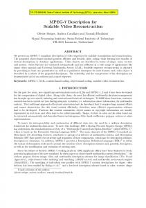
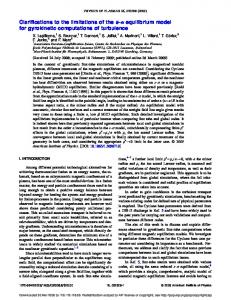
where xh , yh are the states of the oscillator, ωh is its intrinsic frequency, r = p x2h + yh2 and Fx (t) is a perturbing force (the subscript h distinguishes the variables of the Hopf oscillator from variables in the mechanical system). If Fx (t) = 0, this system shows a structurally stable, harmonic limit cycle with √ radius r = µ for µ > 0. It can be shown [18] that such an oscillator adapts to frequencies present in a rhythmic input signal. In the case of a harmonic signal Fx (t) = sin(ωF t) this means ωh is evolving toward ωF . If the input signal has many frequency components (e.g. square signal) the final value of ωh is dependent on the initial condition ωh (0). The size and boundaries of the basins of attraction are proportional to the energy content of the frequency component constituting the basin of attraction, see [18] for further discussion of the convergence properties. Our adaptive frequency oscillators have many nice features which makes them useful for applications and a good example for the dynamical systems approach to learning: 1) no separation of learning substrate and learning algorithm, 2) learning is embedded into the dynamics, 3) no preprocessing needed (e.g. no extraction of phase, FFT, nor setting of time windows), 4) work well with noisy signals, 5) robust against perturbation, 6) they possess a resonant frequency and amplification properties. Now we shall present a few representative results from numerical integration, to show the correct convergence of the adaptive frequency oscillator. First, we show the convergence for a harmonic perturbation Fx (t) = sin(ωF t). As we are interested to show that ωh → ωF , we use ωd = ωh − ωF and φd = φh − φF to plot the results. For all simulations τ = 1, c = 0.1, ωd (0) = 1, φd (0) = 0 and rh (0) = 1. We present results of the integration of the system Eqs. 46. In Fig. 1 the behavior of variables φd and ωd is depicted. In Fig. 1(b), we present the phase plot of the system for the harmonic perturbation. Clearly visible is that the system is evolving towards a limit set. The limit set corresponds to the phase locked case φd ≤ const and the frequency has adapted so that ωd ≈ 0. Since we want to be sure that the convergence works for a wide range of input signals (as in the case when the oscillator is coupled with the mechanical system) we show then results with general nonharmonic perturbation by general TF -periodic functions f (t, ωF ), TF = ω2πF (Fig. 2). The system was subjected to the following driving signals: (a) Square Pulse Signal f (t, ωF ) = rect(ωF t), (b) Sawtooth f (t, ωF ) = st(ωF t), (c) Quadratic Chirp t f (t, ωF ) = cos(ωc t),ωc = ωF (1 + 21 ( 1000 )2 ), (d) Signal consisting of two non-
Preprint May 31, 2005 To appear in Proceedings of the VIIIth European Conference on Artificial Life ECAL 2005 Lecture Notes in Artificial Intelligence (c) Springer Verlag
h i √ commensurate frequency components, f (t, ωF ) = 12 cos(ωF t) + cos( 22 ωF t) , (e) Chaotic signal from the R¨ossler system. There are differences in the convergence speed and in the limit set. Yet, in all cases the oscillators converge to the appropriate frequencies. Very interesting cases are signals with 2 or more pronounced frequency components (such as signals (a),(b) and (d)). In this case the initial condition ωd (0) determines to which frequency the oscillator adapts (cf Fig. 2(d)). The size of the basin of attraction is proportional to the ratio of energy of the corresponding frequency component to the total energy of the signal (due to the lack of space the data is not shown, but can be found in [18]). These simulations show that the adaptation mechanism works despite complex input signals (convergence under broad driving conditions). In the next section we will explore how these interesting properties can be applied to control a mechanical system.
3
The adaptive active spring-mass hopper
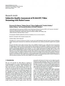
In this section we will present the spring-mass hopper. We will first present the mechanical structure and then focus on the adaptive controller. As a general idea we will exploit the bandpass, and amplification/attenuation properties of both the mechanical system and the adaptive frequency Hopf oscillator. Since our main interest is the adaptation in the controllers, we do not discuss the problem of mechanical stability of the locomotion. We avoid stability problems by an appropriate mechanical structure (wide feet, low center of mass), thus the feet of the robot are wide enough to ensure stability in lateral direction, i.e. the robot is essentially working in a vertical (the “sagittal”) plane. The spring-mass hopper consists of 5 rigid bodies joined by rotational and linear joints (cf. Fig. 3). A prolonged cubic body is supported by two legs. The two legs are identical in their setup. A leg is made of an upper part Mu and a lower part Ml which are joined by a spring-mass system and a linear joint. The function of the linear joint is just to ensure the alignment of the body axes and is otherwise passive. The spring between the two parts of the leg is an activated spring of the form Ff = −kdl , where k = fk (t) and dl is the distance between Mu and Ml . The damper is an ideal viscous damping element of the form Fd = −cd vd , where cd is the damping constant and vd = vu − vl , is the relative velocity of Mu and Ml . The rotational joints between the upper part of the leg Mu and the body Mb are activated by a servo mechanism which ensures that the desired velocity vref is always maintained (cf. [2]). The choice of the spring activation function fk (t) and the choice of the desired velocity vref = fv (t) will be discussed below, when the coupling between controller and mechanical system is introduced. Due to the spring-mass property of the legs the contraction mechanism possesses a resonant frequency ωF 1 . In other words, this type of mechanical system can be interpreted as a band-pass filter with the pass band around ωF . This fact is im1
Note, that the leg can also be considered as a pendulum and thus possesses a second resonant frequency. We will not focus on this intrinsic dynamics in this article.
Preprint May 31, 2005 To appear in Proceedings of the VIIIth European Conference on Artificial Life ECAL 2005 Lecture Notes in Artificial Intelligence (c) Springer Verlag
0.2 0.16
0 2 −4 x 10
0.1
4
6
0.1
8
5
ωd
ωd/ωF
0.15
0 −5 799
799.5
800
0
0
(a) 0
200
400 time [s]
600
800
−3
0 φd
(b)
3
Fig. 1. (a) Integration of the System Eqs. 1-3 (b) corresponding phase plot, in which the frequency adaptation and the phase locking can be seen. 1
1
1
0
0
0
0.5
1
−1 (b) 0 1
0
0.5
1
0
−1 (d)0
5
0 −0.05
time [s]
−1 10 (e) 10 15 20
−0.1 0
0.1
(b)
400
600
800
0
−0.05
−0.05
200
400
600
0.1
(c)
0.05
0
ωd ωF
200
0.1
0.05
−0.1 0
(a)
0.05
−1 (c) not to scale f(t,ω1)
−1 (a) 0 1
0.1
800
(d)
−0.1 0
200
400
600
800
0.1
0
(e)
0.05
−0.1
0
−0.2 −0.05
−0.3 0
200
400
600
800
−0.1 0
200
400
600
800
time[s] Fig. 2. On the top left panel the nonharmonic driving signals are presented. (a) Square pulse (b) Sawtooth (c) Chirp (Note that this is illustrative only since the change in frequency takes much longer as illustrated.) (d) Signal with two non-commensurate frequencies (e) Output of the R¨ ossler system. – We depict representative results on the evolution of ωωFd vs. time. The dashed line indicates the base frequency ωF of the driving signals. In (d) we show in a representative example how the system can evolve to different frequency components of the driving signal depending on the initial condition ωd (0).
Preprint May 31, 2005 To appear in Proceedings of the VIIIth European Conference on Artificial Life ECAL 2005 Lecture Notes in Artificial Intelligence (c) Springer Verlag
Mb Mu
Fore Leg a av
Mu SDh
SDf Ml
(a)Fore Leg
Ml Hind Leg (b)
HO MS
a av
HO Hind Leg
Default parameter values parameter value parameter value µh 0.0001 mb [kg] 0.35 τh [s] 1 mu [kg] 0.09 −1 c [s m ] 0.5 ml [kg] 0.0056 −1 −1 a [N m ] 10 cd [N m s] 0.7 av [rad s−1 ] 10 k0 [N m−1 ] 40
(c)
Fig. 3. (a) The mechanical structure of the spring-mass hopper. The trunk is made up of a rigid body Mb on which two legs are attached by rotational joints. The lower part of the leg is attached by a spring-mass system SD. The lower part consist of a small rigid body. The length of the body is 0.5m (b) The coupling structure of the controller and the mechanical system used for the spring-mass hopper. The upper Hopf oscillator is used for the activation of the fore leg and the lower feedback loop for the hind leg. (c) This table presents the parameters that have been used for the simulations, unless otherwise noted. Note that this parameters can be chosen from a wide range and the results do (qualitatively) to a large extent not depend on the exact values of the parameters. Bottom row: Snapshots of the movement sequence of the spring-mass hopper when the frequency is adapted, i.e. steady state behavior (cf also movie [1]).
portant for the controller to be able to activate the body [4]. This will be further discussed towards the end of this section. The controller of the leg consists of an adaptive frequency Hopf oscillator (Eqs. 1–3), which is perturbed by the activity of the mechanical system (see below for the exact form). The Hopf oscillator acts as a frequency selective amplifier [9], i.e. frequency components of Fx (t) that are close to ωh are amplified. Especially the setting µh = 0 is special in the sense that the system undergoes a fundamental change at that point: For µh < 0 the system exhibits a stable fixed point at z = 0, whereas for µh > 0 a stable limit cycle occurs with radius √ r = µh . This phenomenon is known as a Hopf bifurcation. At µh = 0, there is no signal oscillating at ωh weak enough not to get amplified by the Hopf oscillator. Therefore, for that setting the Hopf oscillator can be considered an ideal amplifier. We use a setting µh ≈ 0. The coupling from the oscillator to the mechanics is established via the spring constants k = fk (t) and desired angular joint velocity vref = fv (t). The oscillator therefore drives both a linear actuator (the spring in the leg) and a rotational actuator (the servo in the hip). The function for the spring constant is chosen as k = k0 + a xrh , where k0 is a constant and a a coupling constant. The function for the desired velocity is chosen as vref = av yh where av is a coupling constant. The choice of this function, which introduces a π2 phase lag between the spring activity and the joint angular velocity is based on the observation of a phase lag between hip and knee joints in locomoting humans and animals. The coupling from the mechanical
Preprint May 31, 2005 To appear in Proceedings of the VIIIth European Conference on Artificial Life ECAL 2005 Lecture Notes in Artificial Intelligence (c) Springer Verlag
system to the Hopf oscillator is established via the relative velocity between upper and lower part of a limb as follows Fx (t) = cvd Fig. 3 illustrates the coupling scheme. Thus, by the coupling scheme a feedback loop is established between the oscillator and the mechanical system. If the resonant frequencies of mechanical system and the Hopf frequency match, i.e. ωF ≈ ωh , an increase of the activity in the system is expected due to the amplifying properties of the Hopf oscillators (cf. [4]). Instead of tuning the controller manually to the appropriate frequency, we let the controller adapt its frequency. In order to achieve this adaptation, we introduce an influence of the mechanical perturbation to the evolution of ωh via an appropriate choice of Fω . Adaptive Frequency The coupling of the perturbation of the mechanical system to the evolution of ωh , allows the controller to adapt to the mechanical system and is equivalent to the perturbation arriving at the oscillator projected on the tangential direction of the limit cycle multiplied with an adaptation rate constant: ω˙ h = − τ1h cvd yrh = − τ1h Fx (t) yrh . This is the same coupling as used for the adaptive frequency Hopf oscillator before.
4
Simulation results
The spring-mass hopper simulation was implemented in Webots, a robot simulator with articulated-body dynamics [15]. In Table 3 we present the parameters for the spring-mass hopper that were used for the simulations unless otherwise noted. Note that this parameters can be chosen from a wide range and the qualitative results do to a large extent not depend on the exact values of the parameters. We first show how the adaptation of the Hopf frequency ωh leads to an excitation of the system and hopping is initiated. To avoid influence of the hip movements on the generated movement the joints are, in this case, fixed at an angle of zero degrees and av = 0, i.e. the hopper is just able to hop in place. Thus, the experiment verifies that the frequency adaptation works. As can be seen in Fig. 4, indeed, due to the adaptation the feet start to lift from the ground. In a next experiment the coupling from the oscillators to the rotational hip joints is set to its default value (av = 10). Due to the activation of the hip joints complex movements emerge. The diversity and self-organization of the movement depends on many factors, therefore in this article we will show preliminary results on the most typical locomotion pattern that was observed. This pattern resembles the bound. The movement sequence of the hopping movement is shown in a series of representative snapshots in Fig. 3. In Fig. 5, the adaptation, feet elevation and displacement of the body is presented. The average achieved velocity in steady state for mb = 0.35 kg is about 0.53 ms−1 (approx. one body length per second). The next experiment shows that the controller correctly tracks changes in the mechanical system. To demonstrate this adaptation capability the mass of the body Mb is changed from mb = 0.2 kg to mb = 0.4 kg at time t = 40 s. The results are presented in Fig. 6. As the mass is changed, the controller immediately starts to adapt and settles after about 50 s to the new resonant frequency. When looking at the displacement of the body xb it is evident that the change in the
Preprint May 31, 2005 To appear in Proceedings of the VIIIth European Conference on Artificial Life ECAL 2005 Lecture Notes in Artificial Intelligence (c) Springer Verlag
(a) ωh [rad/s]
ωh [rad/s]
12 11 10
yh [m]
0
10 0.03
(b)
0 0.03
(c)
yh [m]
0.01
(c)
(a)
12
yf [m]
yf [m]
(b)
14
0
0.01
20
40 time [s]
60
xb [m]
(d)
0
80
50
0
18
0.44
17
0.42
16
(b)
yf [m]
(c)
0
(d) xb [m]
150
0.38
0 0.01
0.36 0.34 0.32 0.3
50
0.28 0.26 10
0
100 time [s]
0.4
(a)
yf [m]
15 0.01
50
Fig. 5. Simulation results of the springmass hopper when the rotational joints are activated a) The frequencies of the Hopf oscillators ωh b,c) Foot elevation yf,h d) Displacement of the center of mass of the body xb . The adaptation of the frequency is clearly visible. As can be seen in the feet elevation measurements and the displacement of the body this adaptation enhances the activity of the leg and initiates a displacement of the body. Interestingly there is a burst of activation (arrow) which increases the adaptation speed before the system settles to steady state behavior.
efficiency ρ
ωh [rad/s]
Fig. 4. Simulation results of the springmass hopper when the rotational joints are not activated. a) Evolution of the intrinsic frequencies of the Hopf oscillators ωh . Note that the frequencies of both oscillators nearly coincide and therefore only one seems visible. b) Fore limb foot elevation. c) Hind limb foot elevation. The adaptation of the frequency is clearly visible and as can be seen in the feet elevation measurements the activity of the system is increased as hopping starts at around 20 s (arrow). The dashed line depicts the theoretical resonant frequency of the spring-mass system when it would not leave the ground. Due to the lift-off of the feet the real resonant frequency is smaller than the calculated value.
50
100 time [s]
11
150
Fig. 6. Test of the adaptation capability of the controller when the mass is changed. At t = 40 s (dashed line) the mass of the body Mb is changed from mb = 0.2 kg to 0.4 kg. See text for discussion.
12
13
14
15
ωh
16
17
18
19
20
Fig. 7. Efficiency ρ vs ωh . See text for the definition of ρ, details of measurement and experimental protocol. The dashed line indicates the frequency to which the oscillators adapt. It is clearly visible that this corresponds to the maximum of the efficiency.
Preprint May 31, 2005 To appear in Proceedings of the VIIIth European Conference on Artificial Life ECAL 2005 Lecture Notes in Artificial Intelligence (c) Springer Verlag
mass slows down the system for a moment but due to the adaptation the velocity is increased again (cf also movies of the experiments [1]). The average velocity before change of mass is about 0.68 ms−1 . After the change, when reached steady state behavior again, the velocity is in average 0.49 ms−1 . In a last experiment we investigate the efficiency of the hopper for forward v locomotion. We define the efficiency as the ratio ρ = Px,b i.e. the ratio between Σ
average forward velocity v x,b of the body and the average power P Σ consumed by all activated joints. In order to assure steady state measurements, the learning is disabled (τh = 0) and the experiment is repeated for different Hopf frequencies ωh = [10, 10.5 . . . , 20]. The transient behavior is removed before the efficiency is measured. In Fig. 7, the results of the efficiency measurements are presented. The line indicates the frequency to which the system evolves if τ 6= 0, thus it is clear that the adaptive frequency process finds the optimal efficiency. It is worth noting, that this optimum in efficiency does not correspond to the maximum of power consumption nor the maximum of velocity (data not shown). This is in line with the observations on animals.
5
Discussion
When introducing adaptation into a system it is important to investigate the convergence properties of the adaptation mechanism. From the mathematical point of view adaptivity on one hand and convergence and stability on the other hand are somewhat opposing requirements. We have shown, that the adaptive frequency oscillator can be driven with general, nonharmonic signals and still adapts to the frequency of the signal. We have presented a 4-DOF spring-mass hopper with a controller based on adaptive frequency Hopf oscillators which adapts to mechanical properties of the hopper. This adaptation has the effect that the spring-mass system starts to resonate and initiates hopping locomotion, similar to the bound. The adaptation is embedded into the dynamics of the system and no pre-processing of sensory data is needed. The system shows fast adaptation to body properties. The results presented in this paper show that with a simple control scheme, it is possible to initiate complex movements and to adapt to the body properties which are important for this movement. In order for this simple scheme to be successful it is important that the controller exploits the natural dynamics of the body. This is in line with observations in nature, where the controllers are found to be complementary to the bodies they control. In fact the adaptation can be considered a type of Hebbian learning as it maximizes the correlation between the signal perturbing the oscillator and the activity of the oscillator. Interestingly, there is no direct coupling between the controllers for the hind and the fore limb. The only coupling between the two controllers is via the mechanical structure and the environment. Nevertheless, an efficient inter-limb coordination emerges and a fast, efficency-optimal locomotion is established. This is interesting as there is no explicit notion of velocity in the system, so it is surprising that the system optimized on velocity/power efficiency.
Preprint May 31, 2005 To appear in Proceedings of the VIIIth European Conference on Artificial Life ECAL 2005 Lecture Notes in Artificial Intelligence (c) Springer Verlag
Immediate possible applications of such adaptive nonlinear dynamical systems are e.g. modular robotics, micro robots, robots which are difficult to model, and adaptive Central Pattern Generators (CPG) for legged locomotion. Furthermore, it will be interesting to explore the use of such adaptive systems in other fields such as in Physics, Biology and Cognitive Sciences, where oscillators are widely used model systems. Acknowledgments This work is funded by a Young Professorship Award to Auke Ijspeert from the Swiss National Science Foundation (A.I. & J.B.) and by the European Commission’s Cognition Unit, project no. IST-2004-004370: RobotCub (L.R.). We would like to thank Bertrand Mesot for constructive comments on earlier versions of this article.
References 1. Movies of the spring-mass hopper are available at http://birg.epfl.ch. 2. Open Dynamics Engine Documentation. available at http://ode.org. 3. R. Blickhan and R.J. Full. Similarity in multilegged locomotion: bouncing like a monopode. Journal of Comparative Physiology, 173:509–517, 1993. 4. J. Buchli and A.J. Ijspeert. A simple, adaptive locmotion toy-system. In S. Schaal, A.J. Ijspeert, A. Billard, S. Vijayakumar, J. Hallam, and J.A. Meyer, editors, Proceedings SAB04. MIT Press, Cambridge, 2004. 5. M. Buehler, R. Battaglia, R. Cocosco, G. Hawker, J. Sarkis, and K. Yamazaki. SCOUT: a simple quadruped that walks, climbs, and runs. In Proceedings ICRA, volume 2, pages 1707–1712, 1998. 6. J.G. Cham, J.K. Karpick, and M.R. Cutkosky. Stride period adaptation of a biomimetic running hexapod. Int. J. of Robotics Research, 23(2):141–153, 2004. 7. J.J. Collins and S.A. Richmond. Hard-wired central pattern generators for quadrupedal locomotion. Biological Cybernetics, 71(5):375–385, 1994. 8. M. de Lasa and M. Buehler. Dynamic compliant quadruped walking. In ICRA 2001, volume 3, pages 3153–3158, 2001. 9. V.M. Egu´ıluz, M. Ospeck, Y. Choe, A.J. Hudspeth, and M.O. Magnasco. Essential nonlinearities in hearing. Phys Rev Lett, 84(22):5232–5235, 2000. 10. Y. Fukuoka, H. Kimura, and A.H. Cohen. Adaptive dynamic walking of a quadruped robot on irregular terrain based on biological concepts. The International Journal of Robotics Research, 3–4:187–202, 2003. 11. R.J. Full and D.E. Koditscheck. Templates and anchors: neuromechanical hypotheses of legged locomotion on land. J Exp Biology, 202:3325–3332, 1999. 12. H. Geyer, A. Seyfarth, and R. Blickhan. Spring-mass running: simple approximate solution and application to gait stability. J. Theor. Biol., 232(3):315–328, 2004. 13. F. Iida and R. Pfeifer. ””Cheap” rapid locomotion of a quadruped robot: Self-stabilization of bounding gait”. In F. Groen et al., editor, Intelligent Autonomous Systems 8, pages 642–649. IOS Press, 2004. 14. H. Kimura, Y. Fukuoka, and A.V. Cohen. Biologically inspired adaptive dynamic walking of a quadruped robot. In From Animals to Animats 8. Proceedings SAB’04, pages 201–210. MIT Press, 2004. 15. O. Michel. Webots: Professional mobile robot simulation. Int. J. Adv. Robotic Systems, 1(1):39–42, 2004. 16. J. Nishii. A learning model for oscillatory networks. Neural Networks, 11(2):249–257, 1998. 17. M. Raibert and J.K. Hodgins. Biol. Neural Networks in Invertebrate Neuroethology and Robotics, chapter Legged Robots, pages 319–354. Academic Press, 1993. 18. L. Righetti, J. Buchli, and A.J. Ijspeert. Dynamic Hebbian learning for adaptive frequency oscillators. Physica D, 2005. submitted. 19. G. Taga. A model of the neuro-musculo-skeletal system for anticipatory adjustment of human locomotion during obstacle avoidance. Biol. Cybernetics, 78:9–17, 1998. 20. K. Tsuchiya, S. Aoi, and K. Tsujita. Locomotion control of a multi-legged locomotion robot using oscillators. In 2002 IEEE Intl. Conf. SMC, volume 4, 2002.
Preprint May 31, 2005 To appear in Proceedings of the VIIIth European Conference on Artificial Life ECAL 2005 Lecture Notes in Artificial Intelligence (c) Springer Verlag