A Fast and Highly Accurate Path Delay Emulation Framework for Logic-Emulation of Timing Speculation Shuou Nomura, Karthikeyan Sankaralingam, Ranganathan Sankaralingam1 University of Wisconsin-Madison, Madison, USA 1 Cadence Design Systems Inc., San Jose, USA Email: {nomura, karu}@cs.wisc.edu,
[email protected]
Abstract This paper proposes a novel path-delay fault emulation technique called Replay. We specifically show it allows FPGA emulation of digital ICs that adopt timingspeculation techniques. For each flip-flop, Replay builds a timing-error predictor based on timing-speculation’s aggressive clock period. We use a heuristic which replicates the combination logic and uses path delays to determine which paths will be excited based on the aggressive clock period. The timing-error prediction accuracy is more than 99% for a set of real workloads on the OpenRISC processor and the FPGA emulation speed shows practically no slowdown. We also demonstrate that Replay can evaluate the impact of voltage-drop timingfaults. This fast and accurate timing-error prediction enables practical emulation of timing-speculation and quantitative analysis early in the design-cycle.
1.
Introduction
Due to non-ideal technology scaling and aging effects VLSI circuits and systems designers must embed considerable design guardband to prevent any timing failure for future microprocessor designs. To minimize this design guardband, timing-speculation (TS) techniques have been recently proposed [1]-[5]. They draw on the insight that signal arrival time to timing elements (flipflops) strongly depends on input patterns applied to circuits and worst-case conditions rarely occur. Thus, they allow aggressive adaptive voltage and frequency scaling optimized for the common-case execution and use a mechanism that can detect/correct rare timing errors that occur during worst-case conditions. To understand the usefulness and quantify the impact of TS in real processors, a practical metholodgy is required for emulating TS at design-time. For a given design and its representative workload, we must estimate how often the worst-case condition occurs and how effectively TS operates the circuit in the common-case condition. Considering a digitial circuit as made up of individual flipflops and combinational logic, we require: A technique that predicts on a cycle-by-cycle basis, whether TS results in an error on any flip-flop. However, conventional static timing analysis (STA)
techniques do not support such analysis. Statistical static timing analysis (SSTA) techniques are more accurate and estimate the distribution of the worst-case timing across different manufactured chips. They cannot evaluate TS techniques, since they do not consider the input data dependency of signal arrival time. Finally, functional simulation and emulation is not aware of timing information and delay-aware annotated functional simulation is very slow. Thus, we need a different framework that allows analysis for common-case behavior to evaluate the effectiveness of TS for various input patterns and environmental parameters like supply voltage and temperature. Such a technique must satisfy the following three criteria. 1) Accuracy: It must be accurate in estimating the potential timing errors due to TS. Under- or overestimation of TS errors will result in inaccurate assessment of the performance and power cost associated with TS. 2) Speed: It must allow fast analysis for various input patterns and environmental parameters. 3) Flexibility: It must be flexibile and allow varying of the TS boundary (aggressive clock period) to quantify the impact of how aggressively timing-speculation can be applied. FPGA emulation is fast and allows representative workloads to be analyzed for large designs. It is already used for different types of fault analysis including gatelevel modeling for single event upsets, stuck-at faults, and transition faults. Stuck-at faults, for example, can be emulated by simply fixing a node to VDD or VSS, and the area complexity is acceptable for full-design emulation [6]. To make TS practial, our approach is to develop support for TS evaluation in FPGA emulation. We call this technique Replay and it satisfies the three criteria described above. Our basic idea is to create a representative logic block (a predictor) that captures and emulates the timing behavior of the original logic when running at an aggressive TS clock period. Our technique employs a prediction heuristic derived from the following observations. First, every input node of a gate can be considered to hold the value from the previous cycle until new inputs arrive in a cycle resulting
Paper 21.3 INTERNATIONAL TEST CONFERENCE 978-1-4244-4867-8/09/$25.00 ©2010 IEEE
1
in computation. Here, a predictor must essentially determine when to use a previous or new value to propagate it to the subsequent logic stages. If all pathdelays[7] through an input node are below the TS boundary, then it will evaluate to the correct new value. Else, it will hold on to its previous value (In the interest of simplicity, we have described the node as “holding” the previous value. In reality, the node triggers computation based on the previous value). In our Replay algorithm, we attach the correct value for such non-violated input nodes of logic gates, while others are computed from the last cycle’s start-point values. Replay improves upon techniques that have been proposed to provide high accuracy and speed. Compared to startpoint-based approximation [8], which ignores all internal circuits, Replay is an order of magnitude more accurate. Compared to path-excitation detection [9], it is several orders of magnitude lower in area complexity. While the focus is on making the analysis for TS practical, our Replay approach provides a general mechanism for emulating path delays with combinational logic in FPGA. It can be used for studying timing-errors caused by voltage-drop, wear-out etc. as well. In this paper, we present the algorithm, describe its integration into the CAD tool-flow, and show results from our prototype implementation of the technique. Our results show that Replay provides more than 99% accuracy in predicting timing errors in TS for a set of real workloads running on the OpenRISC processor. Meanwhile, that of the conventional startpoint-based approximation is about 40%. Replay also allows fast FPGA emulation of timingfault behavior; it is 300,000× faster than delay-annotated gate-level simulation. The remainder of this paper is organized as follows. Section 2 reviews the fundamentals of TS and Section 3 describes TS emulation. Section 4 presents our Replay techniques, Section 5 compares to previous approaches, and Section 6 presents quantitative evaluation. Section 7 shows extensions beyond fine-grained TS, and Section 8 concludes.
2.
Primer on Timing-Speculation
The motivation of TS is to remove or reduce design guardband required for conservative design using the worst-case conditions in determining the clock period. Static techniques like frequency binning and per-die voltage assignment and control can eliminate the margin when the maximum frequency is not necessary. However, they cannot eliminate safety guardband, and cannot exploit arrival time dependency on data, environmental parameters, and aging effects, which are growing in importance. Figure 1(a) shows the basic concept of TS. It uses an aggressive clock period namely TS boundary, which is
Paper 21.3
Timing-Speculation Boundary Aggressive Clock Endpoint Value (Common Case) Endpoint Value (Worst Case) Timing-Error
Worst-Case Arrival Time
(a) Waveform error rate
operation point
worst-case arrival time timing speculation energy optimal point boundary (around 1% error rate) operation range
(b) Operation
Figure 1. Concept of timing speculation. shorter than worst-case arrival time. In the common case, the arrival time is shorter than TS boundary, and it does not cause any timing errors. In case the arrival time is longer than the TS boundary for a given input, an error detection mechanism detects the timing-error, and the recover phase re-executes it with a longer clock-period. The Razor flip-flop implements TS at fine-grain [1] while the Paceline architecture implements a similar idea at coarse-grained processor level [4]. Figure 1(b) shows how to determine the TS boundary. There is an optimal point in terms of energy consumption. If the TS boundary is too long, it cannot eliminate design guardband. If it is too short, the error rate is high, and the performance and power overhead associated with recovery becomes high. In TS techniques, some feedback scheme (hardware only or with software help) observes the error rate and adjusts the TS boundary to set the operation point at the optimal error rate. However, a fundamental problem is that the TS boundary corresponding to the optimal error-rate depends on the circuit and applications. Thus far, researchers have estimated this for individual datapath elements like adders and multipliers. Others have built prototype systems that show 50% power reduction [2] or 20% frequency increase [3] can be achieved. These quantitative results are specific to prototype designs and provide no guidance on how the benefit translates to other designs. Figure 2(a) shows the state-of-art in the CAD tool-flow in how designers can evaluate and use TS. Only after manufacture is it possible to quantitatively evaluate improvements from TS. Estimating TS error rates on a HDL design or netlist can guide designers early in the
INTERNATIONAL TEST CONFERENCE
2
Original Digital IC RTL Design
Physical Parameter
Logic Simulation
Physical Implementation Manufacturing TS Evaluation
RTL Design
Combinational Circuit
Logic Simulation TS Evaluation
Physical Parameter
Physical Implementation
for each F/F endpoint (and startpoints connected to it)
a) netlist b) STA result
Manufacturing
Combinational Circuit
Emulation Circuit Correct Original Endpoint Value Startpoints Combinational (S) Circuit (C)
Replay Framework
Compare (!=)
TS emulation RTL
(a) conventional
TS Emulation Block (C’)
(b) proposed
Figure 2. Design flow of timing-speculation. design cycle. We propose a tool-flow shown in Figure 2(b). Here, TS emulation is done on a netlist and designers can iterate to improve its benefit or continually understand its benefits with design changes. Note that, TS emulation logic is never part of the manufacturing or physical design flow. The TS emulation logic is similar to verification assertions but is inserted automatically. The ability to estimate these benefits before manufacturing can greatly aid in the practical deployment of TS.
3.
Emulation of Timing-Speculation
Figure 3 shows an overview of our TS emulation (TSE) framework that can simulate TS at RTL level. The two high-level inputs to such a framework are the RTL of the design and a clock-frequency that represents the aggressive TS clock. The output is simulation of the circuit and cycle-by-cycle trace of when errors occur due to TS. In the figure, a digital circuit is abstracted as a set of flipflops with combinational logic. Consider a single startpoint (S), endpoint (E), and the logic in between (C). One way to implement TSE is to develop a sparse representation of C, say C' such that for all inputs, the output of C' matches the logical value that would be available when the circuit C operates at the aggressive TS clock. We call this block the TS emulation block (or TSE block). In the figure, we show a detector unit that compares C' to C every cycle and reports when a TS error has occurred. When this reports true, a TS error has occurred, when it reports false, no TS error has occurred. The emulator combined with this simple comparator gives us the TS predictor. The goal of this paper is to develop an algorithm that can produce such representative circuits given the RTL and TS clock as input. In a TSE framework, the three important criteria are accuracy, speed, and flexibility. Accuracy measures how closely to real TS behavior the TS predictor behaves. In evaluating a TSE framework, we have four cases to consider: true positives, true negatives, false positives and false negatives. These can be determined by comparing the TSE framework to a reference TS timing detector (either using a post-manufacture prototype or
Paper 21.3
Predicted Endpoint Value
Endpoint (E) Timing Error Signal
Figure 3. Emulation of timing-speculation. detailed delay-aware simulation). True positive and true negatives are cases when the TS predictor reports true (or false) and the reference TS timing-error detector reports true (or false) respectively. False positives are defined as cases when the TS predictor reports a timing error (true) while in the reference TS hardware no timing error occurs (false). False negatives occur when the TS predictor misses a timing error and reports false, while TS hardware detects this error with a true. The goal of a TS predictor is to minimize both false positives and false negatives. To build effective TS predictors, we draw inspiration from prior approaches from path-delay testing and path-delay emulation [10][11]. In path-delay testing, the circuit is analyzed with timing information, and the goal is to develop inputs to the circuit that sensitize different timing paths, such that functional correctness is violated if there is a timing error. For TS prediction, we use this same insight, but create a single representative circuit that captures the behavior of the circuit up to the aggressive TS clock boundary instead of creating a set of test inputs. This is more complex than path-delay analysis alone because to develop an effective predictor we need to keep track of values from the “previous” cycle to correctly emulate a race behavior between the arrival times of values and the fast TS clock.
4.
Replay Framework
This section describes our Replay algorithm and how it can be implemented in a logic synthesis, static timing analysis, and FPGA emulation framework.
4.1.
Algorithm
Figure 4 shows an abstract circuit and its corresponding Replay generated TSE block to illustrate our basic insight. Our key insight is that the longest path-delay represents the delay of all paths through an input-node of a gate and an endpoint. We explain the algorithm by describing how it constructs the TSE block.
INTERNATIONAL TEST CONFERENCE
3
30
Original Logic
Startpoints
Startpoint A
(functionally incorrect for simplicity) 5ps 15 30
35
Endpoint
40 5ps Startpoint B
40 10ps
40 10ps
40
5ps
Endpoint
40 10ps
arrival time of longest path through this input-node =10+5+10(toward endpoint) + 10+5(toward startpoint)
met paths
(a) Original gate-net with timing information
Met Input-Node Replacement FF FF FF TS Emulation Block
Original Endpoint
Endpoint (predicted)
Original Logic
(one endpoint is shown for simplicity)
TSE Block P
FF
Figure 4. Replay algorithm
R Q
1) We perform STA on the original gate-net to determine path delays for different endpoints. 2) For each endpoint, the original combinational logic is replicated to form the logic part of the TSE block. 3) The startpoint signals of the logic part of TSE block are the previous cycle’s startpoint signals, resulting in a logically redundant module that is one cycle behind the original. 4) Based on the provided TS boundary and the pathdelay analysis, we modify the input nodes of some gates in the TSE block. If the arrival times of all paths through an input node and the endpoint are earlier than the given TS boundary, the node is tied to the original. Here, the endpoint value of the TSE block is the predicted speculation value. Figure 5(a) shows an example circuit with the delay of each gate and the maximum path delay of each input node of the gates. This path delay is the sum of delays of gates that feed into this input and delays of gates driven by that gate. Figure 5(b) shows the circuit with the TSE block when the TS boundary is 32ps. Here, input nodes of three gates (P, Q, and R) are replaced because their maximum delays are less than 32ps, and the replaced gates emulate logical masking behavior for the prediction of the endpoint value, in contrast to the startpoint-based approximation approach as shown in later. The core advantage of this algorithm is that it can represent cumulative mask probability. For the example in Figure 5, the probability that the endpoint is not masked by met paths is the product of non-mask probability in gate Q and that in gate R. Replay simulates this behavior accurately as the actual circuit works, and this lowers false-positive rate, which is important for TS emulation as described above. Note that most gates are common among TSE blocks, and a logic synthesis for FPGA emulation often removes the redundant circuits although the number of TSE blocks is the same as that of endpoints. Thus, our technique results
Predicted Endpoint
FF
(b) Prediction circuit when timing-speculation boundary is 32ps
Figure 5. Example of Replay algorithm. in only a small growth in logic complexity as shown in Section 6.5. Replay was motivated by designing an emulation framework for TS. What we developed in the end is a general and universal technique for timing-aware emulation with combinational logic.
4.2.
Implementation
Figure 6 shows how our Replay algorithm can be integrated with a standard CAD tool flow. Logic synthesis generates the gate-net on which we run a timing analysis step to determine the maximum arrival times for every combination of endpoints and input nodes of logic-gates. These delays are input to the Replay TSE Generator, which outputs an RTL that predicts the endpoint value based on the given TS boundary. For each gate, it compares the path delay on each port and TS boundary to decide if that Original RTL
Logic Synthesis / P&R
Gate Net
STA Results
TS Boundary Replay TSE Generator (This Work) TS Emulator Block RTL
Logic Simulation / FPGA Functional output
Timing-error trace
Figure 6. Tool flow of Replay framework.
Paper 21.3
INTERNATIONAL TEST CONFERENCE
4
port must be connected to the original circuit or left as is. The delay analysis through STA and the generation of the predictor logic modules are performed only once for a given TS boundary. In a typical CAD flow, we expect this generator to be embedded in an STA tool. During functional emulation, the violation of the TS boundary will be determined only through the logical value of the TSE block for applied input patterns. No individual gate delay calculations are required during emulation. Flexibility: Replay can generate prediction RTL for any arbitrary TS boundary without any restrictions. Hence, it can satisfy one of the three required criteria of flexibility shown in Section 1.
4.3.
Computational Complexity of STA
We discuss below the computational complexity of embedding this technique into an STA tool. Here we are considering the complexity of generating the TSE block. The actual logic simulation or emulation of the netlist with the TSE block shows practically no slowdowns. Consider a circuit with e endpoints. For every endpoint, the fan-in tree (n nodes) can be represented as a directed acyclic graph rooted at start-points. We consider the reverse topological sorted list of nodes of this graph which will start with the end-point (which can be constructed with O(n) time complexity). This list is serially traversed, and for each node we increment the path-delay of all nodes in its transitive fan-out by the node’s gate-delay. This phase is also O(n) time complexity. This gives the required path delays. The total time complexity is O(n*e).
5.
Comparison with Past Approaches
Figure 7 shows the startpoint-based approximation [8], which is the only other proposed solution that can realize full-design path-delay fault emulation on FPGA. The main idea of this technique is that timing errors occur at an endpoint only when the value of at least one violated startpoint changes (the violated startpoint means the startpoint that contains at least one timing-violated path to the endpoint). It implements value change detector for every violated startpoint, and the endpoint holds last
cycle’s value when any of startpoint values change. The complexity is low enough for full-design emulation because the number of violated startpoints and endpoints only affects the complexity. However, the accuracy of the startpoint-based approximation is low because of two reasons. First, the error injection scheme on endpoint of holding last cycle’s value is a rough approximation. This scheme only works when there is no value change at an endpoint before TS boundary, and it is too optimistic because general waveform at an endpoint contains many value changes before TS boundary like Figure 1(a). The second reason is that it ignores the internal path structure. Generally, the timing-error rate significantly depends on how frequently the timing-violated paths are logically masked by timingmet paths. In contrast to our Replay technique, the startpoint-based approximation cannot take this mask effect into account. For the example of Figure 5, since the maximum path delays of both startpoints are more than TS boundary of 32ps (35ps for startpoint A and 40ps for startpoint B), the value changes of startpoint “A” cannot propagate to the predicted endpoint in one cycle. As a result, the prediction accuracy is not practical for TS emulation because it contains a lot of false-positives as shown in our evaluation results in Section 6. Figure 8 shows the other approach of path-excitation detection [9], which was originally proposed for evaluating delay-testing coverage. It prepares path excitation condition detectors in RTL for violated paths, and realizes very high accuracy. However, the implementation area on FPGA is unrealistic for full-design emulation because it is proportional to the number of paths to be detected. The experimental results in [9] shows that the emulation of 200 paths requires 2× and that of 400 paths requires 3× area resources compared to the original. This limitation is acceptable for the grading of delay-test because it only needs to analyze some longest paths. In contrast, for the emulation of TS, it is necessary to emulate the timing-fault behavior of all paths whose arrival time is later than the given TS boundary, which can be even 0.5× of the worst-case arrival time. Generally, the number of such paths is exponential. In our
Original Logic Startpoints
Original Logic met paths Endpoint 0 (predicted)
0
1
1
Endpoint (predicted)
violated paths
FF
FF FF
FF FF
Figure 7. Startpoint-based approximation [8].
Paper 21.3
Figure 8. Path-excitation detection [9].
INTERNATIONAL TEST CONFERENCE
5
experiment, a 16-bit multiplier has 175 billions of paths. Therefore, this approach becomes impractical for circuit analysis employing TS techniques. Meanwhile, the worst-case area of the Replay TSE block is less than 6× of the original as shown in the evaluation results in Section 6.5. Thus, it is acceptable for the FPGAbased fault-emulation purpose. Note that the TSE block does not introduce any area penalty to the design since it is never synthesized into manufactured hardware.
6.
Evaluation
In this section, we evaluate Replay on two of the three required criteria of accuracy and speed. Section 4.2 discussed flexibility. Speed is evaluated in Section 6.5, and other sections are for accuracy evaluation. Section 6.1 describes the experimental framework and metrics. Section 6.2 evaluates the basic characteristics of the Replay algorithm using the ISCAS85 benchmark circuits. In Section 6.3, we evaluate with OpenRISC running full applications. In Section 6.4, we describe a detailed performance characterization of Replay.
6.1.
Experimental Framework
Original Gate-Net with Back-annotated Delay Test bench
Emulator RTL
Actual Timing-Error
Emulated Timing-Error
Original Logic
Compare and Count
!= TSE Block
(a) Validation block diagram. Emulated Not Error Emulated Error Actual Error A B Actual Not Error C D Actual Timing Error Rate = (A + B) / (A + B + C + D) Accuracy = (A + D) / (A + B + C + D) False Positive Rate = C / (A + B + C + D) False Negative Rate = B / (A + B + C + D) (b) Metrics definition.
Figure 9. Evaluation overview. command, the STA and report analysis consumed about 5 hours. An STA tool implementing the algorithm should consume less time as described in Section 4.3. The maximum memory usage is about 500MB.
report_timing
6.2
ISCAS85 Benchmark Circuits
Figure 9(a) shows our experimental prototype framework. In addition to the emulator RTL, we perform detailed backannotated gate delay simulation to determine accurately when timing-errors occur. We check the timing-error signal from the original gate-net with back-annotated delay and that from the emulator RTL. The actual timing-error signal asserts when the arrival time of a cycle is later than the given TS boundary. The emulated timing-error signal asserts if a predicted value of TSE block is different from the correct value of original logic. We evaluated every endpoint for which the worst-case arrival time is later than the given TS boundary.
We evaluate the basic characteristics of Replay compared to startpoint-based approximation for the ISCAS85 benchmark circuits [12]. To study aggressive and conservative TS, we show the results for TS boundary set to 0.8× and 0.9× of the worst-case arrival time. The input data are random for every startpoint, and the length of the test vector is 64Kcycles. We evaluate the average of the metrics for all endpoints of each benchmark circuit, and we evaluate the geometrical mean of the metrics for the endpoints of overall benchmark circuits in each timingerror rate range (the metric value of 0 is excluded for the calculation of geometrical mean).
Figure 9(b) shows the metrics related to accuracy, which are evaluated for each timing-violated endpoint. Error rate is the ratio of cycles for which the error signal of original gate-net asserts. Accuracy means the ratio of cycles for which the emulated error signal is the same as the actual error signal. We also show false positive and false negative separately. To study flexibility, we look at many circuits and different TS boundaries.
Table 1 shows the evaluation results for each benchmark circuit. Here we report error rate for each end-point. Compared to the conventional startpoint-based approximation, Replay shows significant improvements on the accuracy (about 2×) and the false-positive rate (about 10×) for most benchmark circuits. The accuracy is relatively low in the c3540 and c6288 benchmarks, which are binary-coded decimal arithmetic ALU and a 16-bit multiplier, respectively; both are complex data-path circuits, in which Replay prediction likely misses because of its approximation as described in Section 6.4. Even in these cases, Replay outperforms startpoint-based approximation.
Experimental setup: We used the Synopsys 90nm technology library, Synopsys Design Compiler for the synthesis and the static timing analysis, and Synopsys VCS for simulation. The delay information for the gate-net simulation (.sdf file) was generated by Design Compiler. The timing constraint was tight enough to synthesize all circuits at their maximum operating frequency. The processing resources for evaluating the OpenRISC design are measured on a 2GHz CPU and 64bit Linux. The processing time of the TSE RTL generator itself is very short (about 7sec). Since this experiment used
Paper 21.3
Table 2 shows a summary across all endpoints classified according to error-rate. The results for this table are obtained by running experiments with 0.8× and 0.9× TS boundaries. Very high error rates are not important because a real system would not operate at this point. The range of less than 1% is the typical operating point. In this
INTERNATIONAL TEST CONFERENCE
6
Table 1. Evaluation results with ISCAS85 benchmark circuits (average of endpoints). Benchmark
TS boundary c432 c499 c880 c1355 c1908 c2670 c3540 c5315 c6288 c7552
TimingError Rate (%) 0.8× 0.9× 6.4 4.5 0.3 0.0 9.9 3.1 0.4 0.0 0.2 0.0 3.2 0.8 15.9 2.6 1.0 0.2 33.6 4.7 6.2 1.1
Accuracy (%) Replay 0.8× 94.6 99.3 90.9 99.4 99.5 89.5 75.0 96.9 70.3 90.5
0.9× 99.2 99.0 94.8 99.1 99.1 86.1 77.0 94.4 80.6 92.6
Startpointbased [8] 0.8× 0.9× 53.7 56.5 50.0 50.0 59.9 57.0 50.0 50.0 51.2 52.8 74.3 66.9 61.8 55.2 60.4 58.9 51.9 52.3 55.9 57.1
Table 2. Results for each timing-error rate range (geometrical mean of endpoints). Range of Timing-Error Rate (x) (%) 10 < x