by adding a penalty term that allows the member- ships of each pixel xk to be influenced by its neigh- borhood. The new objective function is defined as. JS = Jm ...
EUSFLAT-LFA 2011
July 2011
Aix-les-Bains, France
A fast fuzzy c-means algorithm for color image segmentation Hoel Le Capitaine and Carl Frélicot Laboratoire Mathémathiques, Image et Applications, Université de La Rochelle, FRANCE
algorithms, focusing on the fuzzy approach. Then, a new initialization of cluster centers is proposed, along with some numerical examples exhibiting its efficiency in terms of both accuracy and convergence speed. Various algorithms incorporating spatial and speeding-up considerations are presented in Section 3, as well as the new Quantized Fuzzy CMeans (QF CM ) algorithm. Numerical experiments showing the superiority of QF CM as compared to state-of-the-art F CM -based segmentation methods are given in Section 4. Finally, some conclusions and perspectives are drawn in Section 5.
Abstract Color image segmentation is a fundamental task in many computer vision problems. A common approach is to use fuzzy iterative clustering algorithms that provide a partition of the pixels into a given number of clusters. However, most of these algorithms present several drawbacks: they are time consuming, and sensitive to initialization and noise. In this paper, we propose a new fuzzy c-means algorithm aiming at correcting such drawbacks. It relies on a new efficient cluster centers initialization and color quantization allowing faster and more accurate convergence such that it is suitable to segment very large color images. Thanks to color quantization and a new spatial regularization, the proposed algorithm is also more robust. Experiments on real images show the efficiency in terms of both accuracy and computation time of the proposed algorithm as compared to recent methods of the literature.
2. Iterative clustering algorithms 2.1. Algorithms Let X = {x1 , · · · , xn } be a n samples data set and assume that each sample xk is represented by a set of p features. A partition of X into c clusters is a collection of mutually disjoint subsets Xi of X such that Xi ∪ · · · ∪ Xc = X and Xi ∩ Xj = ∅ for any i 6= j. Partitions can be represented by (c × n) hard partition matrices U whose general term is uik = 1 if xk ∈ Xi , and 0 otherwise. To get a partition matrix U , one can use the so-called Hard c-Means (HCM ) algorithm which minimizes the within-cluster distances: c X X J= kx − vi k2 , (1)
1. Introduction Image segmentation can be defined as the process of merging pixels having similar features into the same groups, or regions. The segmented image is then the union of distinct groups, where pixels of homogeneous regions are associated to the same groups. Numerous techniques have been proposed in the literature, where color, texture or edges features are used to decribe each group [8]. Only gray level images were considered by early segmentation methods. As color images become the norm in a wider range of applications (e.g. geographical imaging, medical imaging, or video surveillance), and thanks to advancements in both color technology and computation power, the interest of color image segmentation techniques has grown. Among them, we focus on the clustering approach, especially the fuzzy c-means algorithm (F CM , [3]), which is used by many segmentation methods [1, 13, 5, 22, 12]. However, this algorithm requires to initialize the centers of each cluster [10], and is known to be intractable for very large data sets such as color images. In this paper, we propose a new efficient initialization algorithm especially dedicated to the problem of image segmentation. Furthermore, we introduce a novel fuzzy iterative algorithm allowing fast segmentation of images. This paper is organized as follows. Section 2 first recalls some basic knowledge on iterative clustering © 2011. The authors - Published by Atlantis Press
i=1 x∈Xi
where k.k stands for the usual Euclidean distance and vi are the cluster centers gathered into a matrix V for convenience. The objective function can be rewritten as n X c X J= uik kxk − vi k2 . (2) k=1 i=1
In many real situations, overlapping clusters reduce the effectiveness of crisp clustering methods. Ruspini first proposed the notion of fuzzy partition [18], where samples may partially belong to several clusters through the idea of partial membership degrees. Practically, uik ∈ [0, 1] instead of {0, 1}. Some years later, Dunn [6] modified of the objective function (2) by squaring the individual membership degrees. This has been generalized by Bezdek in [3], with a fuzzifier exponent m > 1: Jm =
n X c X k=1 i=1
1074
2 um ik kxk − vi k ,
(3)
σ such that mσ(k) is an ordered and increasing sequence. We propose to split the n relative means as follows. Assuming that the clusters are equally distributed, we uniformly split the n-dimensional vector m into c groups. In other terms, we set c+1 indices, say `0 , · · · `c , such that the c differences (`i − `i−1 ) are roughly equals1 . More formally, each index is given by
Minimization of (3) is generally obtained by an alternating optimization procedure that successively updates the cluster centers V and the partition matrix U using: Pn m k=1 uik xk (4) vi = P n m k=1 uik 1
uik = Pc
�
j=1
kxk −vi k kxk −vj k
�2/(m−1)
(5)
`i = i ∗ bn/cc
where b.c is the floor function. We iteratively build c subsets Si of n as follows
The choice to first initialize a random partition matrix or the cluster centers is let to the user, both being used in the literature. The algorithm stops when the centroids stabilize, i.e. the matrix norm between two successive V is below a given threshold. Equivalently, the entire procedure can be shifted one half cycle, so that initialization and termination is done on U . Naturally, in terms of speed and storage, there are some advantages to initialize and terminating with V . Application to image segmentation consists in taking X as the entire set of pixels xk of an image I, each of them being described by p features.
Si = {`i−1 + 1, · · · , `i }
Ci = σ −1 (Si )
(9)
Finally, each cluster center is computed using: 1 X xj (10) vi = |Ci | j∈Ci
where |Ci | is the cardinality of Ci . The whole Ordering-split centers initialization procedure is summarized in Algorithm 1. Let us show how the
As defined, iterative fuzzy clustering methods do not guarantee a unique final partition because different results are obtained with different initializations of V (or U ). In particular, it has been shown that these algorithms give better results when the initials (U /V ) are sufficiently close to the final partition/centers [10]. However, most of the practitioners initialize in a random manner, which heavily affects the results. Another reason to correctly initialize the cluster centers is that it allows to speedup the convergence, resulting in a more usable algorithm for large scale practical problems. Several methods have been proposed for the initialization of V . However, most of the methods that allow to initialize cluster centers are computationally expensive. For instance, in [11], the method requires to run the HCM algorithm p times on n 1-dimensional samples, and then p times the same algorithm on n p-dimensional samples, which is intractable for large scale data sets. We propose a new, efficient, yet simple, manner of initializing the c cluster centers, that we call Ordering-split. For each p-dimensional sample xk , we define its relative mean by
Algorithm 1 Initialization of cluster centers Require: X: dataset, c: number of clusters 1: procedure Ordering-split(X, c) 2: compute m by using (6) for each k ∈ {1, · · · , n} 3: apply to m the ordering function σ 4: for i = 0 to c do . uniform splitting 5: `i ← i ∗ bn/cc 6: end for 7: for i = 1 to c do . build the subsets 8: Si ← {`i−1 + 1, · · · , `i } 9: Ci ← σ −1 P (Si ) 10: vi ← |C1i | j∈Ci xj 11: end for 12: return V . the matrix of centers 13: end procedure proposed method is efficient compared to a random initialization of the cluster centers. A simple color image (see Figure 1) in the p = 3 components RGB color space, to which we add a Gaussian white noise with various standard deviations s, is used to compose X. The mean computation times over 100 runs of the HCM algorithm (for simplicity) are reported in Table 1. Note that the time needed for the computation of initial cluster centers is obviously added to the clustering time. We also report the cluster centers proximity index (CCPI) defined by ? − vij 1 X X vij (11) CCP I = , ? vij c×p
p
1X xkj p j=1
(8)
We obtain the subset of indices in each cluster by applying the inverse function:
2.2. Centroids initialization
mk =
(7)
(6)
so that we obtain the n-dimensional vector m = (m1 , · · · , mn ). Note that we are working on features coming from each channel of an image so that the scale of individual features does not differ. If the features do not hold this property, a normalization is required. Let σ be the permutation function
i
1 Note
j
that other hypothesis could be provided, where some information about the clusters distribution is used.
1075
xk . The balance parameter α allows to control the effect of the neighboring terms. However, computing the neighboring terms in each iteration is computationally expensive. Moreover, tuning α is not easy, because a slight variation of α produces very different segmentations. This algorithm is denoted FCM_S in the sequel. In [13], the authors propose another objective function where the relationship between neighboring pixels is taken into account. The usual Euclidean distance between pixels and centers by a weighted mean distance of the pixel and its neighbors to each center is taken. However, here again, in each iteration, all the pixels of the image are considered, leading to a large computation time. In [5], the authors propose to reduce the computation time of the solutions derived from (12) by computing in advance the mean value of the pixel within the specified window:
Figure 1: A 500 × 600 (i.e. n = 300, 000) color image, with Gaussian white noise (s = 0.1). Table 1: Comparison of centers initialization: total time needed for initialization + clustering, proximity and accuracy. time (sec.) CCPI Accuracy s = 0.05 Random Ordering-split
1.286 0.578
0.729 0.088
98.33% 98.33%
JS1 = Jm + α
1.870 0.787
0.714 0.118
92.18% 92.27%
(13)
2.776 1.670
0.787 0.181
53.13% 65.90%
where xk is the mean of neighboring pixels in the window around xk . Additionally, they propose another objective function JS2 where xk is the median value of the neighboring pixels. Then, they introduce the use of kernel-induced distances instead of the usual Euclidean one. The corresponding algorithms are respectively denoted as KFCM_S1 and KFCM_S2 in the sequel. More recently, Yang and Tsai [22] propose to adapt the balance parameter α of (13) to each cluster, namely αi :
s = 0.5 Random Ordering-split
2 um ik kxk − vi k
k=1 i=1
s = 0.1 Random Ordering-split
n X c X
which measures the degree of closeness between the cluster centers V obtained by the initialization algorithm and the desired cluster center V ? . Clearly, the less the CCPI, the better the result. We finally give the accuracy performance defined by the ratio of correctly labeled pixels over the total number of pixels. According to Table 1, we see that the Ordering split method allows to obtain a faster algorithm (time), with an output that is more close to the reality (CCPI), and producing a higher accuracy than the method which consists in randomly initializing cluster centers.
JG = Jm +
(14)
Moreover, since they use kernel-induced distance, they also propose to automatically set the parameters of the Gaussian kernel. The corresponding algorithm is claimed to be a generalized version of KFCM. Here again, the authors allow to consider mean-based or median-based spatial filtering. The derived algorithms are respectively denoted as GKFCM_S1 and GKFCM_S2 in the sequel. Finally, in [12], the authors propose another modification of the objective function somewhat similar to (12) as follows
3.1. Spatial FCM algorithms Whilst the conventional FCM algorithm works well on noise-free images, it is very sensitive to local irregularities, which occur very often in real images. This sensitivity is due to the absence of consideration of the spatial context of each pixel. In [1], Ahmed et al. modify the original objective function by adding a penalty term that allows the memberships of each pixel xk to be influenced by its neighborhood. The new objective function is defined as
k=1
2 αi um ik kxk − vi k
k=1 i=1
3. Clustering for image segmentation
n c α XX m X uik JS = Jm + kxr − vi k2 NR i=1
n X c X
JF L = Jm +
n X c X
Gik
(15)
k=1 i=1
where the penalty term Gik is defined by X 1 Gik = (1 − uij )m kxj − vi k2 , ds (k, j) + 1 j∈Nk ,k6=j
(16) where ds (k, j) is the spatial Euclidean distance between pixels xj and xj .The obtained corresponding updating functions are called FLICM. Naturally, FLICM suffers of the same high computation time as all the previous algorithms.
(12)
r∈Nk
where NR is the cardinality of Nk , which stands for the set of neighbors in a window around the pixel 1076
the authors proposed the bilateral filtering procedure, which is an anisotropic approach based on both spatial and photometric considerations. Formally, the filtered image I 0 is obtained by P j∈N w(i, j)xj 0 (20) xi = P i j∈Ni w(i, j)
3.2. Speeded up clustering algorithms The main drawback of such iterative clustering algorithms is their running time. In [7], the authors propose a fast and accurate clustering method of images. The time reduction is operated by aggregating similar examples and using the weighted prototype in the clustering, giving the brFCM algorithm. In order to speed up the segmentation, Szilagyi et al. [19] used the idea of Eschrich et al. [7] to propose the EnFCM algorithm, which consists in applying the brFCM algorithm to a smoothed image as follows. They first construct a linearly-weighted sum image with local neighbors of each pixel as follows: X α 1 xi + xj (17) xi0 = 1+α NR
where w(i, j) are the weights applied to every pixel xj in Ni . The weights are decomposed by a conjunction into two weights corresponding to the spatial and the color weights, w(i, j) = ws (i, j) × wc (i, j). For instance, in [20], ws and wc are respectively defined by � d2 (i, j) � ws (i, j) = exp − s 2 2σs � d2 (x , x ) � i j (21) wc (i, j) = exp − c 2σc2
j∈Ni
where Ni is the set of neighbors of the pixel xi , and the parameter α controls the influence of the neighbors. Instead of considering each pixel of the image, the objective function uses the number of gray levels in the image, which drastically reduces the computation time, since the number of gray levels of an image is generally much lower than the number of pixels. In [4], Cai et al. propose an improvement of the EnFCM algorithm by adding a local similarity measure Sij . The new image to be clustered is then defined as P j∈N Sij xj 0 (18) xi = P i j∈Ni Sij
In fact, the proposition of [4] consists in adding a bilateral filter process before the clustering algorithm. It can be shown that (20) reduces to (18) if we use ds = L∞ and dc = L2 , where Lp stands for the p-norm. Extending the gray level algorithm [19] to color spaces is not immediate. If we use the same resolution, and take the RGB space, it would lead to compute U and V 28 ∗ 28 ∗ 28 = 224 times. In other terms, this would be equivalent to run the usual fuzzy c-means algorithm on a (4096 × 4096) color image. Since this is computationally intractable in practice, we propose to use a color space quantization into qi bins, i corresponding to the channel index. Most of the color spaces use three channels, so that we have to define q1 , q2 and q3 . Obviously, this can be extended to any multi spectral images, or images where several color spaces are used to describe each pixel (e.g. RGB, HSV and CIE L ∗ a ∗ b∗). In the sequel we consider that each color component is divided into the same number of bins: q1 = q2 = q3 = q. Various studies have shown that many color spaces proposed for computer graphic applications are not well adapted to image processing. As pointed out in [2], a convenient representation should yield distances and provide independence between chromatic and achromatic components. For this reason and comparison purpose, we use the CIE L ∗ a ∗ b∗ color space. There is another advantage of quantizing the L ∗ a ∗ b∗ information rather than RGB information. If L ∗ a ∗ b∗ is approximately uniformly distributed, then a uniform quantization yields a constant distance between any two quantization levels, resulting in small variation of perceptual color difference. This is not the case with RGB data where this variation can be very large. Therefore we define the new objective function to be minimized as
where Sij is a factor incorporating the spatial and gray level relationships in the neighborhood of i. They propose various definitions of the local similarity measure. The first one is given by � ( � kxi −xj k2 − if i 6= j exp − dsλ(i,j) 2 λg σi s Sij = 0 if i = j (19) This similarity measure leads to the FGFCM algorithm. They also propose two other local similarity measures, that we denote FGFCM_S1 and FGFCM_S2. The corresponding similarity measures are respectively defined by Sij = 1 for all i and j, so that xi is equal to the mean of the neighbors, and Sij = median(I(j)), so that xi is the median value of the neighbors. EnFCM, FGFCM and their variants provide quite good segmentation. However, they heavily depend on the internal parameters λs and λg , or α. Moreover, to the best of our knowledge, they are restricted to gray level images, and there are no propositions dedicated to color images. We propose to extend these approaches to color images by color quantization. 3.3. Fast quantized fuzzy c-means
JQ =
Nowadays, processing an image without preprocessing and regularization is pointless. In [20],
q X q X q c X X
2 hq1 ,q2 ,q3 um i,q1 ,q2 ,q3 kxq1 ,q2 ,q3 −vi k
i=1 q1 =1 q2 =1 q3 =1
(22) 1077
where k.k is a convenient norm in the quantized space, e.g. the Euclidean one. For convenience, we rewrite the objective function as
cannot be done in each updating step, so that U is smoothed when the local optimum has been reached. The resulting algorithm, that we call QFCM, is given in Algorithm 2.
3
JQ =
q c X X
2 hl um il kxl − vi k .
(23)
Algorithm 2 Quantized Fuzzy C-Means (QFCM) 1: procedure Segmentation(Image I, No. of clusters c, No. of bins q) 2: Pre-process the image I using (20). 3: initialize cluster centers V using the Ordering-split procedure (Algorithm 1). 4: repeat 5: Update partition matrix U using (24). 6: Update prototypes matrix V using (25). 7: until kV − Vold k < � . k.k is a matrix norm. 8: Regularize the partition U using (26). 9: return (U, V ) . Partition and centers. 10: end procedure
i=1 l=1
Since the gradient of JQ with respect to uil and vi vanishes when P reaching the local optimum, and knowing that i uil sums up to one for all l, it is easy to show that the optimal updating equations of U and V are given by kxl − vi k−2/(m−1) uil = Pc −2/(m−1) j=1 kxl − vj k and
Pq3
vi = Pl=1 q3
hl um il xl
l=1
hl um il
(24)
(25)
Although the introduction of a bilateral filtering process before clustering improves the effectiveness of segmentation, it still lack enough robustness and neighborhood importance should be taken into account in the clustering algorithm. To this aim, we propose, instead of considering the entire image, to regularize the partition matrix, based on the neighborhood of each pixel. The advantage of this proposition is to get rid of the selection of the crucial balance parameter α in the methods of [1, 7, 5, 22]. This parameter ensures a balance between robustness to noise and effectiveness of preserving details. Hence it is hard to set and have considerable impact on the performances. However, due to quantization, the elements of the partition matrix do not have spatial relationships. To overcome this problem, we introduce a mapping of the quantized partition matrix of size (c × q 3 ) to the usual partition matrix of the pixels, of size c × (m × n), where m and n are the width and the height of the image. The basic idea of this mapping is, from a given pixel of the image, to obtain its corresponding bin, say li , in the quantized space. Then, this pixel inherits from the membership degrees of li obtained by u.li . In order to avoid ambiguities, an element of the usual partition matrix is denoted uik , while an element of the quantized partition matrix is denoted uil . Each element of the regularized partition is obtained by rik (26) uik = Pc j=1 rjk
4. Results and comparison 4.1. Performance measures The first measures of evaluation of segmentation were subjective, and the ever growing interest in this topic leaded to numerous metrics allowing proper evaluation. In order to objectively measure the quality of the segmentations produced, 4 evaluation measures are considered in this paper. The first one is the Probabilistic Rand Index (PRI, [21]). This index compares results obtained from the tested algorithm to a set of manually segmented images. Since there is not a single correct output, considering multiple results allows to enhance the comparison and to take into account the variability of human perception. The PRI is based on a soft nonuniform weighting of pixel pairs as a function of the variability in the ground-truth. The ground-truth set is defined as {G1 , G2 , · · · , GL } where L is the number of manually segmented images. Let S be the segmentation provided by the tested algorithm, liGk the label of pixel xi in the k-th manually segmented image and liS the label of pixel xi in the tested segmentation. Then, PRI is defined by P R(S, Gk ) =
X � 2 c pijij (1 − pij )1−cij , N (N − 1) i,j,i