A fast Gauss transform algorithm for the finite element solution of nonlocal integral models Elena Benvenuti, Antonio Tralli Dipartimento di Ingegneria, Universit` a di Ferrara, Ferrara E-mail:
[email protected] Keywords: Fast algorithm, integral equations, non-local elasticity SUMMARY Originally developed for fast solving multi-particle problems, the Fast Gauss Transform (FGT) is here applied to non-local finite element models of integral type (FEFGT). The focus is on problems requiring fine geometry discretization, as in the case of solutions that exhibit high gradients or boundary layers. 1. INTRODUCTION Fast-multipole methods have been developed by Greengard and Rohklin for the direct evaluation of integral equations (Greengard and Rohklin, 1987) and have been successfully applied in the past to a broad range of applied physics problems and to the boundary element solution of heterogeneous materials (Fu et al., 1998; Akaiwa et al. 2001). The Fast Gauss Transform (FGT) is a particular fast-multipole method for the numerical solution of integral equations with a Gauss kernel (Greengard and Strain, 1991). The Fast Gauss Transform replaces the evaluation of the Gaussians at a point with a Hermite polynomial expansion. While direct evaluation of Gaussians over a set of N quadrature points would require N×N operations, the FGT makes the computational cost proportional to 2N. As a new application of the FGT algorithm, the case of non-local elastic materials is here taken into account. In mechanics, the need for non-local models can be adduced on physical and computational grounds. Local continuum models present some pathological effects due to the lack of a material length-scale. In constitutive laws of non-local elastic type, the stress at a point is assumed to depend not only on the strain at the current point but on the strain of the surrounding points, weighted through a distance-dependent weight function, such as the Gauss function or the kernel e−s/` (e.g. Eringen 1981, 1987; Sztyren 1982; Polizzotto 2001). As a consequence of assuming a non-local stress-strain law, a characteristic length is brought into the model. On the other hand, the equilibrium equation becomes an integro-differential equation, where the weight function plays the role of a spatial kernel. Here, a method is proposed for the finite element solution of non-local elasticity problems, that combines the robustness of conventional finite element programs with the superior performance of the fast Gauss transform (FEFGT). The advantages of the FEFGT over traditional FE method are illustrated by comparing the computational time by varying the number of the polynomial components. It is shown that the saving-time capacity of the FEFGT method is 1
significant whenever a fine discretization of the geometry is required. In this case, satisfying results can be obtained by taking few terms in the Hermite expansion with a significant reduction of the computational time. Examples are reported concerning a one-dimensional tensile bar in non-local elasticity for both the Gauss kernel and the kernel e−s/` . This contribution stems from a recent work of the authors on the subject (Benvenuti and Tralli, 2005), which also contains an extensive discussion of the numerical results obtained for the case of a previously developed non-local damage model (Benvenuti, Borino, Tralli 2002). 2. THE FAST GAUSS ALGORITHM Because closed-form solutions of linear integral equations are not always available, computational methods to solve linear integral equations are therefore essential, based on suitable discretization procedures. Let us consider a discretization grid made of N evaluation points xj with j = 1, . . . , N , associated to wj weight coefficients. The discrete version of an integral quantity weighted through the Gauss function can be written as: G(x) =
N X
w j e−
|x−xj |2 `2
(1)
j=1
In the terminology of fast-multipole mathematics, the centres of the Gaussians x j are also called sources, while the evaluation points x are called targets. The sum of all the Gaussians generated by the N sources at each target xj , with j = 1, . . . , M : M X i=1
G(xi ) =
M X N X
wij e−
|xi −xj |2 `2
(2)
i=1 j=1
has to be evaluated. Following (Greengard and Strain, 1991 ), the sum of the weighted Gaussians (2) can be calculated by means of the Hermite series +∞ X |x−xi |2 Φn (x − s)Ψn (xi − s) (3) e − `2 =
where
n=0
µ ¶n ¶ µ |xi −s|2 1 x−s xi − s Φn (x − s) = (4) , Ψn (xi − s) = e− `2 hn n! ` ` |x−xi |2 Equation (3) describes the Gaussian field e− `2 at the target x due to the source xi as a Hermite expansion centered at an arbitrary point s. In expansion (3), the Gauss function, which depends on (x, xi ), is expressed as the product of the function Φn , which depends on x, and the function Ψn , which only depends on xi . Such a separation of variables is a key-feature of the fast Gauss algorithm. Direct evaluation of the sum at the M targets over N sources therefore requires M × N operations. The fast Gauss algorithm makes the computational cost to be proportional to the sum M + N . In the one-dimensional case, the starting point for the fast Gauss algorithm is the definition of the Hermite functions n 2 2 d (5) (e−t ) hn (t) = (−1)n et n dt and the generating Hermite polynomials 2
1
1
−x2 /`2 0.9
e
0.8 0.7
0.5
0.6 0.5 0.4
0
0.3 0.2 0.1 0 −1
−0.5
0
x[mm]
0.5
−0.5 −1
1
−0.5
0
x[mm]
0.5
1
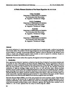
Figure 1: A) One-dimensional Gauss function centred at x = 0 with ` = 0.3 calculated by direct evaluation (red dotted line) compared with its fast Gauss approximation (continuous line); the Hermite expansion is shifted to s = `/2 and arrested at the first 5 Hermite polynomials; B) One-dimensional Hermite polynomials Φn (x − s)Ψn (xi − s), with n = 0, . . . , 4 .
2
e2xs−s =
∞ X sn hn (x) n! n=0
(6)
where s is an arbitrary point. As usual, the function sign(x) is positive for x positive and negative for x negative. Figure 1A displays the approximation of the FGT of a one-dimensional Gauss function centered at x = 0 over a set of points {xi } ranging over the adimensional closed set [−1, 1]: the Gauss function calculated by direct evaluation (red dotted line) is compared with its FGT approximation (blue continuous line). The approximation was performed as follows: the Hermite polynomials were shifted to s = `/2, where ` was set equal to 0.3, and expanded up to p = 5 terms. Figure 1B displays the first five component polynomials Φn (x − s)Ψn (xi − s), n = 1, . . . , 54, adopted for Figure 1A. . 3. NON-LOCAL ELASTICITY FE MODELS Let us consider a body of volume Ω and boundary ∂Ω, where each particle at the position x ∈ Ω is characterized by the strain ²(x). A certain distribution of forces and prescribed displacements is assumed. In the Eringen model of non-local elasticity, the non-local actions that the material particle x exchanges with the surrounding ones can be taken into account by defining a non-local stress of the type Z g(x, y)C(y)²(y) dΩy (7) σ ¯ (x) = Ω
3
where the function g(x, y) denotes a weighting function. According to Eringen (1987), Polizzotto (2001), the constitutive stress-strain lawZ (8) σ(x) = ξC(x)²(x) + ξ¯ g(x, y)C(y)²(y) dΩy Ω is here analyzed, where ξ and ξ¯ are positive material constants. Assuming ξ + ξ¯ = 1, constitutive law (8) can be read as the stress-strain law of a mixture of a local phase and a non-local phase. Constitutive law (8) make it possible to obtain the local and the non-local behavior as limit cases for ξ or ξ¯ tending to 1, respectively. Owing to its simplicity and physical meaning, the most used weighting function in non-local elasticity is the Gauss function g(x, y) = g0 (x)e−
|x−y|2 `2
(9)
where ` denotes an intrinsic length. The factor g0 (x) normalizes g(x, y) either over the infinite domain or over the finite body. |s|
3.1 THE FGT FOR THE KERNEL e− ` Analytical solutions would be highly desirable to correctly identify the features of the solution. While closed-form solutions of boundary value problems in non-local elasticity are not available for the Gauss kernel, an exact solution was derived by Pisano and Fuschi (2003) for the equilibrium problem of a one-dimensional tensile bar of length L subjected to a constant |s| non-local stress σ ¯ defined by Equation (8), where the kernel is g(s) = g 0 e− ` . In the case of a one-dimensional tensile bar with homogeneous Young modulus and unit cross-section A, constrained at one end, and subject to a prescribed load N = A¯ σ daN at the free, assuming the normalization factor g0 = (2`)−1 , the closed-form solution reads · ¸ λx`−x x−L λ` ²(x) = ²¯ − ²¯ e ` + eλ(L−x) e ` (10) 2 ¯ −ξ where λ = and ²¯ = σ ¯ /E. It can be shown that the strain solution defined by Eq. (10) 2`ξ exhibits a boundary layer at x = 0, L . The mathematical features of non-local boundary value problems were investigated for this specific kernel, for instance, by Sztyren (1982). A generalization of the FEFGT algorithm to the non-Gaussian kernel e− To this purpose, it can be written √ |x−xi |
−
|x−xi |2 √
` e− ` = e The generalization of the Hermite expansion (3) becomes
e−
|x−xi | `
=
+∞ X
n=0
Φn (x − s)Ψn (xi − s)
where the component polynomials turn out to be p µ ¶n |x − s| 1 √ sign(x − s) Φn (x − s) = n! ` p µ ¶ −|xi −s| |xi − s| √ Ψn (xi − s) = e ` hn sign(xi − s) ` 4
|x−xi | `
, is carried out. (11)
(12)
(13a) (13b)
Therefore, all the relationships necessary for the implementation of the FGT-based approximation of the kernel e−s/` are available. 4. FINITE ELEMENT FORMULATION FOR NON-LOCAL ELASTICITY In this section, the solving system of algebraic equations is considered for the non-local material defined by Equation (8) following the standard procedure of the finite element method (Bathe, 1996). The domain is accordingly discretized into Ne finite elements. The finite element representation of the displacement field u is based on the map ue (x) =
ne X
ϕi (x)Ue i
(14)
i=1
where ϕi (x) denotes the shape function corresponding to the i-th element degree of freedom, Ue i , with i = 1, . . . , ne . In small strain displacements, the associated strain, defined as the symmetric part of the displacement gradient, ²e = ∇s ue , becomes ne X ∇ϕi (x)Uei (15) ²e (x) = i=1
After collecting the shape functions ϕi in matrix Ne (x) and introducing the compatibility operator ∇Ne (x) := Be (x). Equations (14) and (15) can be cast in the compact form ue (x) = Ne (x)Ue , ²e = Be (x)Ue (16) where the vector Ue collects the nodal displacements of the element e. After assembling the element contributions, the displacement and strain over the global domain become u(x) = N (x)U,
²(x) = B(x)U
(17)
In the following, symbols where the index e has been dropped will identify global variables. Let us suppose that, after straightforward computations, the usual algebraic system of equilibrium equations KU = F (18) is found, where F denotes the nodal force vector. The global stiffness matrix K is written as: K=
Ne Z ^
k=1
Ωk
Btk (x)C(x)Bk (x) dΩk
(19)
V Ne where k=1 denotes the assembly operator and Ωk indicates the domain of the k−th element. The stiffness matrix K can be expressed as the sum of two terms: ¯ K = ξK + ξ¯K
(20)
¯ indicates the non-local contribution to the stiffness matrix. The local matrix K in where K turn results from the assembly of the element stiffness matrices Z (21) Btn (x)C(x)Bn (x) dΩx Kn = Ωn
5
The non-local stiffness matrix ¯ = K
Z Z Ω
Ω
g(x, x0 )Bt (x) C(x) B(x0 ) dΩx0 dΩx
(22)
where the weighting function g(x, x0 ) is the Gauss fuction, results from the assembly of the elementary stiffness matricesZ Z ¯ nm = K g(x, x0 )Btn (x) C(x0 ) Bm (x0 ) dΩn dΩm (23) Ωn Ωm as follows Ne Ne ^ ^ ¯ nm ¯ = K (24) K m=1 ¯ nm expresses the influence ofn=1 The matrix K the stiffness of the m element on the n element. The non-local stiffness matrix possesses an imbricated structure: each element stiffness matrix derives from the weighted sum of the stiffness matrices of the surrounding elements.
To perform numerical integration, a set of Nq quadrature points is identified in each finite element, leading to a total number of Nq × Ne quadrature points. As usual, a Gauss-Legendre integration rule is adopted. The generic quadrature point qnk of the element n with k = 1, . . . , Nq is associated to the weight of integration wnk . In the simple case of one-dimensional elasticity, ¯ nm defined in Equation (23) is calculated through the direct evaluation the stiffness matrix K of the Gaussians at the quadrature points. A description of the standard FE procedure follows. Let us set for the sake of brevity µ ¶ ¯ ¯ K(n, m) K(n, m + 1) ¯ nm := (25) K ¯ + 1, n) K(n ¯ + 1, m + 1) K(n The usual finite element procedure that can be followed for the case of linear displacement interpolation is hereby reported. For each finite element n for each quadrature point qnh of the element n, h = 1, . . . , Nq , for each finite element m, m = 1, . . . , Ne , k for each quadrature point qm of the element m, k = 1, . . . , Nq , evaluate the stiffness contributions ¯ nm + wh wk g(q h , q k )Bt (q h )EB(q k ) Jm Jn (26) K m n n m n m
Equation (26) calculates the stiffness coefficients, that couple the degrees of freedom n and n+1 of the initial and final nodes of the element n, with the degrees of freedom m and m + 1 of the initial and final nodes of the element m. The symbols Jn and Jm denote the Jacobian of the change of variable required by the Gauss-Legendre numerical integration relative to the n− and m−elements, respectively; in the one-dimensional case, Jk = l2k , with lk denoting the length of the k−element. The standard FE procedure consists of Ne × Nq × Ne × Nq evaluations. When a 6
large number of finite elements Ne and of quadrature points Nq is necessary to obtain accurate results, a direct evaluation of the Gaussians can be computationally too expensive. 5 FEFGT ALGORITHM FOR 1D NON-LOCAL ELASTICITY In this section, the Fast Gauss algorithm is combined with the finite element method. The target and source points of the multipole context are now identified with the quadrature points of the finite element mesh, while boxes B now coincide with the finite elements. Moreover, according to Greengard and Strain (1991), the fact that the Gaussian function decays at a certain distance ρ` from the actual point is exploited. Therefore, the actual number of evaluations is reduced. Let 2n + 1 be the number of elements that contain quadrature points whose distance from the actual point is less than ρ`. For simplicity, linear one-dimensional finite elements are assumed. The FGT algorithm for non-local FE elasticity is given by the following sequence of logical steps:
Step 1 For each finite element n, n = 1, . . . , Ne , for each quadrature point qnk , k = 1, . . . , Nq , evaluate the stiffness matrix Nq X n wnk g0 (qnk )B(qnk )t EB(qnk ) Jn Φα (qnk − cn ) Kα = k=1 is the
where α = 0, . . . , p, cn normalization condition.
(27)
centre of the element n, and g0 (qn ) fulfils the adopted
Step 2 For each finite element n, n = 1, . . . , Ne , for each quadrature point qnk , k = 1, . . . , Nq , of the element n for each element j such that j = 1, . . . , Nj , evaluate the non-local stiffness coefficients as p X ¯ nj = K ¯ nj + (28) K wnk Kjα Jn Ψα (qnk − cj ) α=0
where cj is the centre of element j, and Nj = 2n + 1.
where ¯ nj := K
µ
¯ K(n, j) ¯ + 1, n) K(n
¯ K(n, j + 1) ¯ + 1, j + 1) K(n
(29)
Equation (27) in Step 1 transforms the Gaussians evaluated at the quadrature points of the element n into an expansion shifted to the center cn of the element n. As a consequence, the 2 × 2 stiffness matrix Kαn stores the non-local stiffness contributions emanating from each finite element n. Subsequently, these element stiffness contributions are used in Step 2 to evaluate through Equation (28) the global stiffness coefficients, that couple the degrees of freedom n and n + 1 of the initial and final nodes of the element n, with the degrees of freedom j and j + 1 of 7
the initial and final nodes of the element j. The cost of the operations required in Step 1 is proportional to Ne × Nq × p evaluations, while the operations of Step 2 are Ne × Nq × (2n + 1) × p. The total computational time is therefore proportional to O1 = (Ne × Nq × p) + (Ne × Nq × (2n + 1) × p). A standard FE format, where those Gaussians emanated at distances larger than ρ` are truncated, would instead require O2 = Ne × Nq × (2n + 1) × Nq evaluations. The relative efficiency of the FEFGT method over O1 p the FE method can therefore be expressed through the ratio ≈ , which, in the present O2 Nq analysis, is always less than 1. 6. EXAMPLES A bar of length L = 100 cm, unit cross-section A, and Young’s modulus E = 2.100.000 daN/cm 2 constrained at one end, and subject to a prescribed load N = A¯ σ = 100 daN at the free end is considered. For the sake of simplicity, the displacement is interpolated through linear Lagrangian functions, and finite elements of the same length and meshes with 5 or 7 quadrature points were used. In particular, 5 points were used for values of the parameter ξ¯ ≤ 0.5 and 7 points otherwise. The FGT algorithm is independent of the adopted normalization condition of the Gauss function. However, in this section, the normalization factor is g 0 = (`π)−1 . −5
16
x 10
l=2 l=5 l=10 l=20
14 12 10 8 6 4 2 0
20
40
60
80
100
Figure 2: FEFGT: strain profiles obtained with ` = 2, 5, 10, 20 mm, p = 1, using 100 finite elements, and setting the non-local parameter ξ¯ = 0.9.
To better highlight the `−dependence of the results, the strain profiles obtained through the FEFGT approach with ξ¯ = 0.9 were then compared and are shown in Figure 2 for ` = 2, 5, 10, 20 mm. It can be observed that the boundaries of the strain profiles are particulary sensitive both ¯ It should be noted that the strain at the bar to ` and to the value of the non-local parameter ξ. centre attains the same value ²¯ = A σ ¯ /E = 4.7619 × 10⁻⁵ , corresponding to a homogeneous strainFEFGT state. algorithm was implemented on PC Matlab platform supporting a Pentium IV The processor. Tables 1 and 2 compare the CPU times in seconds necessary to calculate the nonlocal stiffness with the FEFGT and with the FE model. Table 1 compares the CPU times 8
N = Ne × Nq 100× 5 100× 5 100× 5 100× 5 100× 5 100× 5 100× 5 100× 5
` 2 5 10 20 2 5 10 20
p 1 1 1 1 3 3 3 3
FEFGT 1.25 1.30 1.35 1.5 3.72 4.03 4.02 3.69
p 2 2 2 2 4 4 4 4
FEFGT 2.97 2.51 2.98 2.47 4.99 4.98 4.98 4.97
FE 7.43 7.96 8.06 9.13 7.43 7.96 8.06 9.13
Table 1: FEFGT versus FE: comparison of the CPU times ([s]) for calculating the non-local stiffness ¯ setting p = 1; the results have been obtained by truncating the influence of elements placed at a K distance greater than 20`.
N = Ne × Nq 500 × 5 400× 5 400× 5 100× 5 100× 5 100 × 5 100 × 5 40 × 5
` 2 1 2 1 2 4 20 2
FEFGT 7.56 6.12 5.94 1.46 1.26 1.47 1.27 0.45
FE 45.3 35.65 34.04 6.76 7.46 8.06 8.04 1.96
R 0.17 0.17 0.17 0.21 0.17 0.18 0.16 0.23
Table 2: FEFGT versus FE: comparison of the CPU times ([s]) for calculating the non-local stiffness setting p = 1; the calculations have been performed by truncating the evaluations of the finite elements placed at a distance greater than 20`.
9
employed to calculate the non-local stiffness with the FEFGT, arresting the Hermite expansion at various p terms and for various non-local lengths `. The number of quadrature points per each element were fixed equal to Nq = 5, and 100 finite elements were used in Table 1. These results were obtained by truncating the influence of elements placed at a distance greater than 20`. It should be noted that the CPU time slightly increases with `, because the number of quadrature points inside the influence zone increases. In Table 2, the Hermite expansion has been arrested at the first term p = 1. The results were obtained by truncating the evaluations of the finite elements placed at a distance greater that 20`. For the sake of clarity, Table 2 reports the parameter R that denotes the ratio between the CPU time required by the FEFGT algorithm and the CPU time required by the FE format. The FEFGT-based algorithm implies a CPU time which is 16 ÷ 23% of the CPU time required by a standard FE method. On the other hand, when the discretization is coarse, the number p of the Hermite polynomials to be accounted for increases, and the FEFGT algorithm can be less convenient than direct evaluation. s
The case of the non-Gaussian kernel e− ` is next considered. A comparison between the computed FE strain profile (dashed line), the FEFGT profile (continuous line) and the analytical profile (dash-dotted line) can be evinced from Figure 3. The results were derived using 500 finite elements, ξ¯ = 0.9, ` = 10 mm, and taking into account p=1 Hermite polynomials, as it has been verified that a larger p leads to the same results. The FE and the FEFGT profiles provide very similar results, and the largest error, with respect to the analytical solution, is as expected located at the boundaries.
−5
x 10
14 12
²
10 8 6 4 0
20
40
60
x[mm]
80
100
Figure 3: Kernel e−s/` : comparison between the analytical solution (blue-dash-point line), the FEM strain profile (red-dashed line), and the FEFGT strain profile (green-continuous line) obtained for ξ = 0.1, l=5 mm, and using 500 FE.
10
7. CONCLUSIONS Developed for numerically solving integral equations, Fast multipole methods were successfully applied in the past to a broad range of applied physics problems (Greengard and Strain, 1991), and to the boundary element solution of heterogeneous materials (Fu et al., 1998; Akaiwa et al. 2001). The Fast Gauss Transform (FGT) is a fast multipole method that can be used for the numerical approximation of integral equations with a Gaussians kernel through a Hermite series. Among the possible applications, a new application, namely non-local elastic materials, is taken into consideration in this contribution. The present analysis makes it possible conclude that, in the case of large scale computations, the FGT applied to the FE framework pursues a satisfying compromise between computational efficiency and accuracy of results. Acknowledgements: Financial support of the PRIN 2003 research project “Interfacial damage failure in structural systems” is gratefully acknowledged. References: Akaiwa, N., Thornton, K., Voorhees, PW. 2001. Large-scale Simulations of microstructural Evolution in Elastically Stresses Solids. Journal of Computational Physics ; 173: 61–86. Bathe, KJ. 1996. Finite element procedures. Prentice & Hall International Editions. Benvenuti, E., Borino, G., Tralli, A. 2002. A thermodynamically consistent non-local formulation, European Journal of Mechanics/A Solids, 21: 535–553. Benvenuti, E., Tralli, A. 2005. The fast Gauss transform for non-local integral FE models. submitted. Eringen, C. 1981. On nonlocal plasticity, International Journal Engineering Science, 12: 1461– 1474. Eringen, C. 1987. Theory of nonlocal elasticity and some applications. Res Mechanica; 21: 313–342. Fu, Y, Klimkowski, KJ., Rodin, GJ., Berger, E., Browne, JC., Singer, JK., van der Geijn, RA., Vegamanti, KS. 1998. A fast solution method for three-dimensional many-particle problems of linear elasticity. Int. J. Num. Meth. Engng. 1998; 42: 1215-1229. Greengard, L., Rohklin, V. 1987. A Fast Algorithm for Particle Simulations. Journal of Computational Physics, 73, 325–348. Greengard, L., Strain, J. 1991. The fast Gauss transform. SIAM Journal of Scientific and Statistical Computation. 12:79–94. Pisano, AA., Fuschi, P. 2003. Closed form solution for a non-local elastic bar in tension. International Journal of Solids and Structures ; 40: 13–23. Polizzotto, C. 2001. Non-local elasticity and related variational principles. Int. J. Solids and Structures; 38: 7359–7380. Sztyren, M. 1982. Solvable nolocal boundary value problem, in : Introduction to nonlocal theory of material media. In Rogula D. Ed., Nonlocal theory of material media. Springer Verlag, Berlin, 223–278.
11