A Fast Parallel Algorithm for Convex Hull Problem of ... - Springer Link
Recommend Documents
In this paper, we propose a parallel algorithm to solve the convex hull problem for an ... Finding the convex hull of an image component or a set of points .... To obtain one of these configurations a PE may set up the corresponding switches.
May 28, 2009 - Informatica 34 (2010) 369-376 369 ... Department of Computer Science, Guangxi Normal University, Guilin 541004, P.R. China. E-mail: ...
Aug 3, 2011 - Also, in Table 1, the numbers of backtracks for both algorithms are ... of the PB algorithm is much less than the backtracks of Skiena's algorithm.
starting and finishing at the same city, that will permit one to visit each ... This research was assisted by the award of an Adelaide University. Research Grant to ...
X-axis, and the point with the minimum coordinate value in the X-axis is needed when the reference axis is Y-axis). As a result, tetragon L D R U. PPPP divides ...
The algorithm has been named the 'Newton Apple ... Newton Apple Wrapper algorithm or 'NAW' algorithm for short) that ..... std::ofstream out(fname, ios::out);.
of angle vector of the point P and every polygon vertex is 360°. When the point P is outside ... 3 Process of convex hull construction. (1) The point L .... such that every triangle's circum-circle contains no other point of S inside it. The edges o
Search algorithm for finding next triangle ABC when the baseline AB is gwen. First (for ... The algorithm presented here assumes as Graham a (conventional).
JOHN HERSHBERGER and SUBHASH SURI ... planar convex hull problem, where h denotes the number of points on the hull. .... Let us define P(v) = P c~ S(v).
for convex optimization problems with known saddle-point structure. ...... man operator splitting method, and split Bregman method can be considered as ...
second round of discarding using SPA, and finally form a simple chain for the current remaining points. A simple ..... stage for outputting. ... Dragon, Happy Buddha, Turbine Blade, Vellum Manuscript, Asian Dragon, Thai Statue, and Lucy.
Proposition 1 is proved. The essence of the above ... CA is the set obtained as the result of Algorithm A. Then. S(Câ. ) .... 79 (1â3), 191â215 (1997). 24. P. Hansen ...
The sequential complexity of computing the convex hull of a set S of n points in
Jul 24, 2013 - this study, we suggest a tabu search algorithm that incorpo- ... greedy algorithms, and the result shows that the tabu search algorithm gives ...
implementation on a cluster of six computers. The experimental ... is to find a processing order of the n jobs, the same for each machine (i.e. passing is .... others frameworks dealing with parallel B&B method in shared and distributed envi-.
dle point can be eliminated as a possible convex hull ... vex hull algorithm given in this paper which have been ..... 2 Potter, J., J. Baker, A. Bansal, S. Scott, C.
image. Now, we'd also like the robot to respond to the orientation of the lightstick. In this ... Add p to the hull. 3. ... 4 Preprocessing a binary image for convex hull.
Given a set of points P (e.g. the big red blob ... 4 Preprocessing a binary image for convex hull ... binary image, the number of (4-connected) neighboring 1's.
of l1 minimization and run very fast on small dataset, they are still computationally expensive for large-scale ... quad
1 Laboratoire de Statistique d'Enqu~te, CREST - ENSAI, rue. Blaise Pascal, Campus de Ker Lann, 35170 Bruz, France. 2 Statistics Group, University of Neuchs.
Nov 22, 2018 - Mathematics Subject Classification 49N45 · 65F22 · 90C25 .... the LâTV model and a fast projection algorithm onto the l1 ball is reviewed.
Jul 7, 2002 - to run under Windows NT 4.0. Energy rules. When calculating the secondary struc ture energy, parametrization was used.15. Sequences.
nonnegative matrix factorization (NMF) with KL divergence, which is proved to ... plain phenomenon in science [3], [6], [12]. ... arXiv:1604.04026v1 [math.OC] 14 ...
Jul 1, 2010 - One topic of recent interest is the convex hull conv(C) of a ... [11, 18], facial structure [17, 23], and volume estimates [3, 19] for such convex bodies. .... convex body P = conv(X) is the projection of the 6-dimensional Hermitian spe
A Fast Parallel Algorithm for Convex Hull Problem of ... - Springer Link
Key words: reconfigurable mesh computer, convex hulls, image processing, parallel ... Finding the convex hull of an image component or a set of points.
A Fast Parallel Algorithm for Convex Hull Problem of Multi-Leveled Images O. BOUATTANE, J. ELMESBAHI and A. RAMI B.P 1151, La Coline Mohammedia, Morocco; e-mail: [email protected] (Received: 22 May 2000; in final form: 6 June 2001) Abstract. In this paper, we propose a parallel algorithm to solve the convex hull problem for an (n × n) multi-leveled image using a reconfigurable mesh connected computer of the same size as a computational model. The algorithm determines parallely the convex hull of all the connected components of the multileveled image. It is based on some geometric properties and a top-down strategy. The complexity of the algorithm is O(log n) times. Using some approximations on the component contours, this complexity is reduced to O(log m) times where m is the number of the vertices of the convex hull of the biggest component of the image.This complexity is reached thanks to the polymorphic properties of the mesh where all the components are simultaneously and separately processed. Key words: reconfigurable mesh computer, convex hulls, image processing, parallel processing.
1. Introduction Several authors have discussed the problem of the convex hull in the recent years. It is a very important problem in image processing domain, pattern recognition and robotic [2, 4]. Finding the convex hull of an image component or a set of points has been solved by several authors using some parallel methods [5, 7, 12]. The proposed algorithms have been assigned to be implemented on many parallel computational models such as the Mesh connected computer [8], Polymorphic Torus [6] and Reconfigurable Mesh computer [3]. In [8] the authors have proposed some solutions for the convex hull using the set of lattice point as the input data of the algorithm at the first time. Then they have discussed the same problem for the n × n digitized black/white pictures. In θ(n) time, the algorithm processes all the components of the image and decide if a component is convex or no. In [6], the problem is viewed as the detection of the extreme points of a unique set of lattice points in order to find the smallest convex polygon enclosing these points. The complexity of this algorithm is O(1) time. The same problem as in [6] was solved in O(log n) times on pyramid and hypercube machines [13]. The recent works as 2 in [3] propose an almost optimal convex √ hull√algorithm running on O(log(log n)) time on a reconfigurable mesh of size n × n. In this paper the problem of Convex Hull (CH) is studied using another approach and other kinds of data. The input of our algorithm in an n×n multi-leveled
286
O. BOUATTANE ET AL.
image stored on a reconfigurable mesh computer of the same size. The problem is to find simultaneously the smallest convex polygons of all the connected components of the image. In this approach the algorithm takes only the component contours as useful data, (i.e., all the computation procedures run on the component contours). Since the image is stored on the reconfigurable mesh one pixel per processing element (PE), we will merely use the terms pixel and PE to designate the same thing. The principal goal of our algorithm is to determine parallely the extreme PEs of each component. The basic tool of the method is the computation of the Euclidean distance separating the PEs of the component contour and a straight line segment. It is a purly geometrical method which detects some extreme PEs of the component at each time. We use a top-down strategy which split the initial rectangle enclosing a component into subrectangles until all the extreme points of a component are detected. The splitting operation is fictitious, i.e., only the contour PEs know the coordinates of their subrectangle vertices, thanks to the reconfigurability of the mesh. The complexity of our algorithm is O(log n) times in the worst case. Using some approximations, this complexity can be reduced to O(log m) times where m is the number of the vertices of the biggest component approximated by straight line segments. This paper is organized in the following manner. Section 2 gives a brief presentation of the computational model and some of its reconfiguration operations used in the algorithm. Section 3 describes the method of the extreme points determination and some of its basic tools. More details concerning the implementation of the algorithm are given in Section 4. Section 4.2 deals with the complexity analysis of the algorithm. Concluding remarks are given in Section 5.
2. Computational Model The model of computation used in this paper is the reconfigurable mesh computer. It is a massively fine grained parallel architecture of n × n, processing elements (PEs) model. The PEs of the mesh are organized in a 2-D matrix where each PE(i, j ) is characterized by its Cartesian coordinates i and j . The reconfigurable mesh is a SIMD structure machine (Single Instruction, Multiple Data), where each PE is connected to its four neighbors if they exist, by a bidirectionnal communication channel (see Figure 1). It is an architecture that was studied by several authors and used in many works as a computational model [1, 9, 10]. Each PE of the mesh can carry out arithmetical and logical operations as well as the reconfiguration operations. Each PE possesses a finite number of registers of size log n bits in which it saves different Data such as, its row and column indices, its identifier which may be in row major, shuffled row major, snake-like or proximity order [11], gray level or color values and so on. The reconfiguration operations performed by the PEs offer the mesh a polymorphic structure where the PEs can communicate with each other in a unit time
CONVEX HULL PROBLEM OF MULTI-LEVELED IMAGES
287
Figure 1. Reconfigurable Mesh computer of size n × n.
whatever their position may be in the n × n matrix. The advantage of the reconfigurability of the mesh in image processing is that it allows a parallel computing of all the connected components of the image, since their separation is based on a channel locking operation that each PE can easily carry out. The other reconfiguration properties may be explored in this paper according to their usefulness and depending on the desired processings so that the algorithms complexities can be reduced in term of number of iterations. Due to the interest of the reconfigurability of the mesh, we will present in more details its different operations. They are classified in three categories named: Simple Bridge, Double Bridge and Crossed Bridge. 2.1. SIMPLE BRIDGE ( SB ) A PE goes into a SB state by linking only two of its communication channels each other. This operation offers several configurations as shown in Figure 2(a). To obtain one of these configurations a PE may set up the corresponding switches to the channels to be linked, e.g., the configuration of Figure 2(a.2) is obtained using the switches of the East and West channels, the others remain inactive. These reconfigurable operations have already appeared in the literature [1, 6, 10], where a given operation takes different appellation from one author to an other. A PE in SB states may be connected to its bridge either in emitter or receiver mode. Also, it can be neither in any of the two modes, which is the inactive mode. 2.2. DOUBLE BRIDGE ( DB ) It is an operation where the four channels of a PE may be groupped into two pairs of channels, each pair constitutes a single bridge. Thus a PE in DB state will have two different Buses which may be configured as in Figure 2(b). A PE in DB state
can be connected in transmitting or receiving or inactive mode, either to one or to both of its buses. In the example of Figure 2(b.2), the PE in DB state creates two different buses; the first is horizontal where it uses the E and W ports, the second is the vertical bus using the N and S ports. This PE can read or write either in the horizontal or vertical bus.
2.3. CROSSED BRIDGE ( CB ) The crossed bridge state is obtained by establishing a single link between the four ports of the PE. The result of a CB state is a single bus where the PE can transmit Data in four directions, it can also receive data from this unique bus. Notice that according to the state of the ports of a PE (locked or unlocked), we can see other configurations as shown in Figure 2(c). When two ports of a PE are locked, the CB state becomes the one of the SB configurations. Notice that the locking and unlocking operations are also considered as the reconfiguration operations. The very important operation that makes use of CB is the direct broadcasting, where a PE can broadcast Data to a set of the PEs in the array in a unit of time. Figure 3 illustrates the direct broadcasting operation between the representative PE and the other PEs in the component A. The required operations are: – All the PEs of the component A go into the CB state, – The representative PE connects itself to the resulted grid in emitting mode, and the other PEs in receiving mode. – The representative PE sends data over the grid from which all the PEs of the component A will receive in a unit of time. More details about the reconfiguration operations in technological point of view and communication cost are discussed in [6], where the polymorphic torus is equipped by the same reconfiguration network as the reconfigurable mesh.
CONVEX HULL PROBLEM OF MULTI-LEVELED IMAGES
289
Figure 3. Direct broadcasting using CB operation.
3. Extreme Points Determination In this paper, the approach used to determine the smallest convex polygons of the different connected components of an image is based on the following principales: • Each component contour is reparted into contour portions, each one delimited by two extreme points with which we can form a segment representing the chord of this portion. • The search of other extreme points is done by the decomposition of these portions into subportions. The extreme points of these subportions will be the (CH) convex hull peaks. • Determining a point of CH on a given portion is done by the method of a projection in relation to its chord. So a point of CH is the farthest point from the chord. • CH point determining process is iteratif and helps to detect at least one CH point in each contour subportion. • The first departure points are those which are delimited by the extreme points of the rectangle enveloping the components. The complexity of the algorithm is O(log n) times on an n × n reconfigurable mesh computer. This complexity can be reduced by approximating the shape of each component by a set of straight line segments. Hence the complexity becomes O(log m) times where m = Max(mi ) and mi is the number of straight line segments aproximating the component of label ‘i’. To develop the method we use the following properties:
290
O. BOUATTANE ET AL.
Figure 4. Euclidean distance between a point of a curve and a segment.
PROPERTY 1. We consider two points A(x1 , y1 ) and B(x2 , y2 ) in an Euclidean plan, the distance between a given point C(xc , yc ) and the segment [A, B] is given by the distance between C and a point P, where P is the projection of C on [A, B], see Figure 4. A(x1 , y1 ) and B(x2 , y2 ) are the extreme points of the segment C(xc , yc ) a given point on the curve and P(xp , yp ) its projection onto the segment [A, B]. We have the following relations: Given a straight line ( ) containing the points A and B. The equation of ( ) is: y = ax + b, where a=
y2 − y1 x2 − x1
and
b=
y1 x2 − y2 x1 . x2 − x1
The point P (xp , yp ) is characterized by its coordinates xp =
In our case A and B stand for the extreme points of a contour portion and C is any point in this portion. PROPERTY 2. Any connected component of an image is delimited by a rectangle of sides passing by at least one extreme point of this component and belonging to its CH.
CONVEX HULL PROBLEM OF MULTI-LEVELED IMAGES
291
Figure 5. Delimitation of a component by a rectangle according to OX and OY axes.
In the example of Figure 5. The points A, B, C and D are the first detected points of the CH. The component contour can be diveded into four portions (A, B), (B, C), (C, D) and (D, A). Their associated chords are respectively the segments [A, B], [B, C], [C, D] and [D, A]. In the euclidean plane we see that: the slopes of [A, B] and [C, D] are 0. PROPERTY 3. In our method a segment of slope null or infinity is a segment of CH (i.e, it belongs to CH).
Illustration of the Method Taking the same example as in Figure 5. We have four rectangles R1 , R2 , R3 and R4 having respectively [A, B], [B, C], [C, D] and [D, A] as diagonals. Running in clockwise order these segments; we can see that, all the points that are susceptible to belong to CH must be placed in the left side of these segments. Hence, each portion point must know its position in relation to its segment (i.e., left side or right side). – The right-side points do not take part in the computation process, because they are located in the concavity zone of the component part. – The left-side points are those taking part in the computation process, because they are in the convexity zone. Thus these points are susceptible to belong to CH.
292
O. BOUATTANE ET AL.
Figure 6. Determination of the PEs of the convexity and concavity regions of a portion contour.
Figure 6 illustrates the concavity and convexity regions in the subrectangle R1 . The same thing goes for all the other subrectangles. In the same figure, for a given rectangle Ri (i = 1–4), if the slope αi of its diagonal is >0, (respectively, 0; where a and b are the diagonal parameters of the quadrant to which the points M belong. These points are those in the quadrants R1 and R4 (see Figure 7). – Category 2 (C2): The points M(X, Y ) of a portion contour such that Y −aX − b < 0; they are the points in quadrants R2 and R3 (see Figure 7).
CONVEX HULL PROBLEM OF MULTI-LEVELED IMAGES
293
Figure 7. Different categories of component contour in the subrectangles.
– Category 3 (C3): The points M(X, Y ) belonging to the portions of the contour but delimited by two extreme points having the same ordinate according to the x-axis or to the y-axis. These point are eliminated from the computation process starting from the first stage (see Figure 7). Before starting each iteration of the algorithm, each point must know to which category it belongs. Thus, the category identification is done at each iteration, and each point keeps its own category until the end of the corresponding iteration. 4. Detailed Description Before describing the different stages of our algorithm, we consider a multileveled image of size n × n stored in a reconfigurable mesh computer one pixel per PE. The image is made of several connected components to which we will parallely determine their convex hull by operating only in their contours. At the end of the algorithm, we can know all the vertices points of the smallest convex polygon of each connected component. Our CH algorithm starts by at least two reference points of the CH. At each stage we detect new points of each CH component. These latters will participate in the succeeding steps in order to detect other CH points. This process is repeated until there are no new CH points. 4.1. ALGORITHM This algorithm is divided into two phases; The first one corresponds to the preprocessing phase, the second phase corresponds to the procedure which determines the peaks of the CH of a component. The peaks are the extreme PEs of the contour and correspond to the vertices of the smallest convex polygon enclosing the component in query.
294
O. BOUATTANE ET AL.
Phase 1 Stage 1: Connected Components Isolation Given an n × n multi-leveled image stored on an n × n reconfigurable mesh computer one pixel per PE. Assuming that the image is segmented, then its different connected components are isolated from each other by performing the following operations: – Each PE compare its gray level with those of its four neighbors. – Each PE locks its communication channels relating it to its neighboring PEs and having the different gray level as its own. – All the PEs of the RMC go to the CB state to establish connexions between the PEs of each component. Figure 3 illustrates the result of this stage. It achieves in O(1) time. Stage 2: Component Centring In this stage, we will determine the covering rectangle of each component. Each rectangle will cross its component on at least two extreme points. These points serve as the departure ones for the CH points search process. The rectangle determination requires the following operations: – Determining in each component the PEs having the smallest row index (Xmin ). This is done using the Min search operation in each component contour. This operation is done in O(1) time as in [6]. – The same thing goes for the determination of Xmax , Ymin and Ymax . Hence we can see in Figure 6. the rectangle construction of an image component. All the contour PEs of each component receive the coordinates of the rectangle reference points of the component. This happens after these coordinate broadcasting in the component contour using the CB operation. This stage is of O(1) time complexity. Stage 3: Categorization of the Contour Portion To assign a given category (as stated above) to a portion contour. We must perform the following operations: 1. All the PEs of the different contour portions go to the SB state, to create the contour channels. 2. In each component contour, each PE having an index Ymin (computed in stage 2.) sends a logical level ‘1’ on its contour channel. According to its location, the logical level ‘1’ is sent in the first time to the portion of its left side, and in the second time, it is sent to its right one. 3. The PEs having received the logical level ‘1’ twice, held the C3 label. They belong to the category C3. All these points are removed from the computation process, because there is no extreme point in this portion (concavity portion).
CONVEX HULL PROBLEM OF MULTI-LEVELED IMAGES
295
Figure 8. Categorization of the component contour.
4. The PEs having received the logical level ‘1’ once, must perform the test corresponding to the category C2, in order to determine the points of the concave part and those of the convex one in the portion in query. The points on the concave part are eliminated and not used until the end of the algorithm, but those of the convex part will participate in the computation process. 5. The operations 1 and 2 are now performed by the PEs having an index Ymax (computed in stage 2). Hence we can find portion which must perform the corresponding tests to the category C1 or C3. In the same fashion as in 4), these will appear the points of the concave part and those of the convex one. Note. It may exist in each rectangle other portions of category C3. They are those delimited by the extreme PEs having the same index Xmin or Xmax . Figure 8 shows the result of all these tests. The PEs having received two logical level ‘1’ are of category C3, those having received logical value ‘0’ belongs to the concavity region, otherwise the PEs are in the convexity region they are the PEs which participate to the selection of the extreme PEs. These latter PEs are shown in Figure 9 performing projections onto the chord of their contour portion to compute the Euclidean distance d 2 . Phase 2: Finding the CH Peaks This stage allows us to find in each rectangle at least one extreme point which will make a part of CH peaks list. This stage requires the following operations: 1. In each portion of the contour, all the active PEs set up the coordinates of its extreme PEs. These extreme PEs are also the extreme points of rectangle diagonal to which they belong. 2. All the inactive PEs remain in the SB state until the end of the algorithm.
296
O. BOUATTANE ET AL.
Figure 9. Separation of the contour points according to their categories.
3. In each contour part, all the active PEs calculate the distance d 2 defined in Property 1. This allows each PE to know the distance separating it from the chord of its portion. 4. Using the Max operation in each portion, we can find the maximal value of d 2 which indicates the farthest PE from the chord. Hence this farthest PE is a detected point of the CH, it take a label CH. Note. During the Max operation, there might appear more than one maximal value of d 2 , then all their corresponding PEs are the points of the CH. 5. In order to progress in the iterative process of the algorithm, all the detected points of CH in the ith iteration will be inserted in the contour as the new extreme points of the new portions of the contour. They transmit their coordinates to the PEs of their portion. Finaly, the (i + 1)th iteration is ready to start from the first stage of the algorithm. This iterative procedure goes on until there remains no active PE in the contour. This means that all the extreme PEs of the CH are detected. Figure 10 shows how the extreme PEs are detected at each iteration. Figure 10(a) corresponds to the first iteration where we detect the first vertices of the CH, the second iteration is illustrated in Figure 10(b) in which we see the new vertices of CH. Finally the third iteration in Figure 10(c) determines the remaining vertices of the CH. Thus each component has the list of all the vertices of its convex hull. Figure 10(d) represents the convex hull of the studied component. 4.2. COMPLEXITY ANALYSIS The complexity of our algorithm corresponds mainly to those of the second phase, since the first one takes O(1) time. For the purpose of evaluating the second phase
CONVEX HULL PROBLEM OF MULTI-LEVELED IMAGES
297
Figure 10. Evolution of the convex hull of a component.
complexity, we will be located in the worst case for which we determine the number of the required iterations. For our method the worst case is an n×n image consisting of one cercle centered on a point C(n/2, n/2) and having a diameter D = n. See Figure 11. In this figure we notice that the algorithm can start with two extreme points A, C or B, D. During the 1st iteration there appear 2 new extreme points. During the 2nd iteration there appear 4 new extreme points. During the 3rd iteration there appear 8 new extreme points. .. . During the kth iteration there appear 2k new extreme points. Hence the process is continued until the iteration N, such that all the points of the considered cercle are detected as the extreme ones. Since the number of point in our circle is 2n. So 2n = 2N , this imply that N = 1 + log n.
298
O. BOUATTANE ET AL.
Figure 11. The worst case figure to which we compute the convex hull.
If we take A, B, C and D as the starting points, then N = log n times. This complexity goes down as the image in query possesses several connected components, since all these components are parallely processed. It can also be enhanced by reducing its number of iterations. We can realize this by reducing the number of points which participate in the computation process. A method of reducing these points use a procedure which approximate the component contour by a set of straight line segments. In this case the resulted number of points is the number of straight line segments of the component or the number of vertices of the polygonal shape approximating a component contour. Then the complexity is O(log m) times where m is the number of the segments approximating the biggest component of the image. 5. Conclusion In this paper we have presented a parallel algorithm to solve the convex hull problem of digitized images. It determines simultaneously the convex hull of all the connected components of an image. The approach used in this algorithm is based on the connected component contours of the image. It is assigned to be implemented on a parallel architecture which is the reconfigurable mesh computer of the same size as the image. The complexity of this algorithm decreases when the image presents several connected components. In the worst case the algorithm achieves in O(log n) times for an n × n image. It fastly decreases when the connected
CONVEX HULL PROBLEM OF MULTI-LEVELED IMAGES
299
component contours are approximated by straight line segments. The fastness of this algorithm is due to reconfiguration operations carried out by the PEs of the reconfigurable mesh computer. References 1. 2. 3. 4. 5. 6. 7. 8. 9. 10. 11. 12. 13.
Elmesbahi, J. and Charkaoui, J.: Structure analysis for Gray level pictures on a mesh connected computer, in: Proc. of IEEE Internat. Conf. on SMC, October 1986, pp. 1415–1419. Fu, A. M. N. and Yan, H.: Effective classification of planar shapes based on curve segment properties, Pattern Recognition Lett. 18 (1997), 55–61. Hayachi, T. et al.: An O((log log n)2 ) time algorithm to compute the convex hull of sorted points on reconfigurable meshes, IEEE Trans. Parallel Distributed Systems 9(12) (1998). Jarvis, C.: Fitting polygons to figure boundary data, Austral. Comput. J. 3 (1971), 50–54. Kim, C. E. and Stojmenovi´c, I.: Parallel algorithms for digital geometry, CS-87-179, Washington State University, Pullman, December 1987. Li, H. and Maresca, M.: Polymorphic torus architecture for computer vision, IEEE Trans. Pattern Anal. Mach. Intelligence 11(3) (1989), 233–242. Ling, T. et al.: Efficient parallel processing of image contours, IEEE Trans. Pattern Anal. Mach. Intelligence 15(1) (1993), 69–81. Miller, R. et al.: Geometric algorithms for digitized pictures on a mesh connected computer, IEEE Trans. Pattern Anal. Mach. Intelligence 7(2) (1985). Miller, R. et al.: Meshes with reconfigurable buses, in: Proc. of the 5th MIT Conf. on Advanced Research in VLSI, Cambridge, MA, 1988, pp. 163–178. Miller, R., Prasanna-Kummar, V. K., Reisis, D. I. and Stout, Q. F.: Parallel computation on reconfigurable meshes, IEEE Trans. Comput. 42(6) (1993), 678–692. Miller, R. and Stout, Q. F.: Mesh computer algorithms for computational geometry, IEEE Trans. Comput. 38(3) (1989), 321–340. Prasanna, V. K. and Reisis, D. I.: Image computation on meshes with multiple broadcast, IEEE Trans. Pattern Anal. Mach. Intelligence 11(11) (1989), 1194–1201. Stout, Q. F.: Mapping vision algorithms to parallel architectures, Proc. IEEE (August 1988).