explicitly make use of the phase-change boundary, and so are free of the restrictions ..... with 130 lines for the explicit enthalpy and previous three-level methods ...
hr. J. Hra/ Mus Twsfrr. Printed in Great Britain
0017-9310/85s3.00+0.00 Q 1985 Pergamon Press Ltd.
Vol. 28. No. II, pp. 2079-2084. 1985
A fast, unconditionally stable finite-difference scheme for heat conduction with phase change Q. T. PHAM Meat Industry
Research
Institute
of New Zealand,
(Receiued 13 November
P.O. Box 617, Hamilton,
New Zealand
1985 and injnaf form 13 May 1985)
Abstract-In the numerical solution of heat conduction problems with phase change by finite differences, enthalpy methods or temperature methods can be used. The former require either an explicit procedure with consequent convergence problems, or iteration at each time step ifimplicit procedures are used. The latter are subject to the problem of jumping the latent heat peak, necessitating the use of small time steps to avoid underprediction of phase-change times. This paper suggests a simple method that eliminates both problems and results in a fast, robust procedure that uses less computation time for the same level ofprediction accuracy
when compared to other finite-differenceschemes.
INTRODUCTION THE NUMERICAL
solution of heat transfer processes with phase change (Stefan problems) presents special difficulties. Numerous methods have been proposed for these problems, as reviewed for example by Fox Cl], Furzeland [2], Crank [3] and Voller and Cross [4]. Of these methods, many can deal only with situations where a sharp phase-change boundary exists and thus do not apply to the freezing of many materials such as solutions, foodstuffs or alloys. Others are restricted to one-dimensional problems. This paper will concentrate on methods which do not explicitly make use of the phase-change boundary, and so are free of the restrictions mentioned above. In these methods, the heat diffusion equation can be formulated in either of the following two ways : a-
c(T) iit
=
. div [/c(T) grad(T)]
c should be calculated as the mean specific heat between the temperatures of adjacent nodes. This method was also followed by Succar and Hayakawa [S]. Apart from thelack of theoretical basis it leads to ambiguities when applied to multi-dimensional situations. Morgan ef al. [9] suggested calculating a mean value of c from the changes in nodal temperatures and enthalpies at the previous time levels, m and m + 1. This represents a departure from the three-level scheme. Also, because the moment when a node changes phase is not anticipated, peak jumping still occurs, unless time steps are very small and the width of thelatent heat peak made artificially large (Morgan et al. found a l”C-width necessary). A further modification suggested by Wood and Lewis [lo] is to change the temperature as follows, when updating at each time step :
(1)
or aH
at
= div [k(H) grad (T(H))].
(2)
Equation (1) is the basis of temperature methods, while (2) is the basis of enthalpy methods. In temperature methods, the latent heat is represented by a peak of small but finite width in the c(T) curve. If a large time step is used in the computation, a nodal temperature may ‘jump’ past the freezing temperature range in one step, resulting in the latent heat being ignored [since c(T) never takes the peak value]. This is termed ‘jumping of the latent heat peak and can be a major problem. To avoid it, very small time steps have to be used. Three-time level schemes such as that of Lees [S] goes some way towards solving this problem (Bonacina and Comini [6]). In these schemes the thermal properties are evaluated at an intermediate time level. However, jumping of the latent heat peak is still likely. To overcome this Comini and Lewis [7] suggested that HNT Lti:Il-G
2079
T:=(T;+2+Ty+1+T:)/3.
(3)
In addition to this, Cleland [ 1l] suggests ‘smoothing out’ the c(T) function around the peak. Cleland and Earle [12] show that to guarantee that the solution is accurate, it is essential to check the heat balance. The smoothing of the c(T) peak leads to predictions of lower accuracy and makes it difficult to carry out checks against known theoretical solutions. Enthalpy methods do not suffer from the drawbacks mentioned above. However, because the heat diffusion equation involves a highly non-linear function T(H) near the phase-change region, an explicit scheme is usually employed : H” + ’ -H”
= f(H”).
(4)
Explicit schemes are unstable for kAt/c(Ax)’ > 0.5. Thus, again small time intervals must be used, with a consequent increase in computing time. Longworth [13] and Furzeland [2] propose implicit formulations of the enthalpy method, which require iteration at each time step to determine thermal properties. Crowley [14] employed both explicit and implicit methods to
2080
Q. T. PHAM
I NOMENCLATURE C
Subscripts
volumetric heat [J rn-’ K-‘1 a function functions to calculate temperature from enthalpy and vice versa enthalpy [J mm31 enthalpy change [J mm31 thermal conductivity number of nodes time interval [s] temperature [K] distance interval [ml.
iA4 H
AH k n At T AX
solve the enthalpy equation and found the latter to be less efficient in terms of computing time. This paper proposes a method that combines the features of enthalpy and temperature methods : better convergence of implicit temperature methods and robustness with regards to peak jumping of enthalpy methods, without recourse to time-consuming iteration at each step. THEORY To facilitate discussion most of the following will refer to one-dimensional problems, although the same principles apply to multi-dimensional problems. Lees’ [ 51 three-level finite-difference equation can be written :
x[km,+‘(~~~+T~,?11+T~+l-T~+2-T~+1-T~) + k’!!- ‘( Ty-+, +T~+11+T;-“_1-T;+2-T;+1-T;)]. (5) This second-order scheme is unconditionally stable and convergent. The RHS gives the enthalpy gain (due to heat conduction) at node i over the time interval Aht.A second-order approximation to this enthalpy gain is :
+k-(Ty?,‘-7-T+‘)]. A second-order approximation
and a second-order approximation ,:+I
AH* = ~, T*-Tim
Unlike previously suggested schemes, equations (6H8) yield a ‘true’ mean specific heat at the second time level. As a further precaution against jumping the latent heat peak, the temperatures Tyf2 are recalculated (after solutions of the tridiagonal matrix) as follows : Tr”(corrected)
to cy+ ’ is : (8)
Thus, CT’ ’ can be calculated from explicity known quantities (at time levels m and m + 1) and substituted into equation (5), which can then be solved in the usual manner, using a tridiagonal matrix solving procedure.
= fT[fH(T))+ c~+~(TY+~ - T;)]. (9)
In equations (7) and (9), the functionsf, andf, are approximated by segmentwise functions. The term in square bracket on the RHS represents the calculated new enthalpy at node i. Thus, if cy’ ’ has been underestimated, causing Ty+’ (incorrectly) to ‘jump’ past the freezing temperature, equation (9) will reset Ty+ ’ to the freezing temperature. The two-step procedure described above in effect transforms the temperature method into an enthalpy method, while retaining the convergence properties of the implicit three-level scheme [since equation (8) is an approximation of the same order as equation (5)]. Extension to two and three dimensions is described by Bonacina and Comini [ 151 and Cleland and Earle [ 161. Essentially it consists of ‘sweeping’ successively in two or three directions. Step 1 (calculation of specific heats) is carried out before the first sweep, and step 2 (recalculation of temperatures) after the last sweep. The increase in computing time due to the two-step modification of this paper is undetectable.
RESULTS
Performance for various specific heat curves Three test problems were set up (Tables 1 and 2). The proposed method was compared with its ‘parent methods’, the explicit enthalpy method and the threelevel temperature method. Two versions of the latter were tested: version II includes the modification of equation (3), while version I does not. Note that the present method does not make use of equation (3) either. Comparison was also made against Longworth’s [13] and Furzeland’s [2] iterative implicit enthalpy methods. The modification suggested by 1.
(7)
cooling medium freezing point spatial index between nodes i and i+l between nodes i and i-l.
Superscripts 111 time index * second-order approximation.
(6)
to Ty+’ is :
T* = fT[fH( T;) + AH*]
f” i + -
A finite-difference scheme for heat conduction with phase change
2081
Table 1. One-dimensional test problems Problem 1 Slab thickness (m) Heat transfer coefficient (W mm2 K-‘) Ambient temperature (“C) Initial slab temperature (“C) Thermal conductivity (W m-r K-r)
0.100 infinite 0 100 0.48
Volumetric heat (lo6 J mm3 K-‘)
3.66
Number of nodes (half slab) Specified final centrej temperature (“C) Known solution (s) (time to given final centref temperature)
10
Problem 2
Problem 3t
0.500
0.025 51.9 -40 30 Table 2
infinite -20 10 2.22, T < -0.005 0.556, T > 0.005 1.162, T < -0.005 33 800, - 0.005 < T < 0.005 4.226, T > 0.005 50
Table 2
5
-1 11755 (theory)
40
8950 (theory)
-10 2300+ 150 (experiment)
t Problem 3 is from Cleland and Earle’s [18] Tylose freezing test No. 1. $ For problem 2: replace ‘centre’ by ‘0.05 m below surface’.
Morgan et al. [9] was also tried, but made little difference to the performance of three-level methods, and its results will not be shown separately. The test problems can be described as a pure cooling problem, a pure-substance freezing problem with step change in enthalpy, and a food-freezing problem with gradual phase change. The theoretical solution to the first problem is given by Carslaw and Jaeger [17, p. 1241. In the second problem, the time for a 0.5-m-thick slab to freeze to a depth of 0.05 m is calculated. For the period considered, the centre temperature remains at its initial value and the half-space solution given by Voller and Cross [4] applies. The third problem has no theoretical solution but had an experimental result of 2300+ 150 s measured by Cleland and Earle [18]. The enthalpy step-change in problem 2 was approximated by a narrow peak 0.01 K wide in the specific heat curve. Strictly speaking such an approximation is not necessary for either the enthalpy method or the present method. However, its use simplifies the programming, since the specific heat
never actually goes to infinity and thus no special feature needs to be built into the program to handle this case. (The peak width can be an arbitrarily small number, as long as the numbers involved can be handled by the computer.) The methods were compared according to the following criteria : Time interval At at which the calculated cooling or freezing time agrees to within 1% with the true result (i.e. result obtained when very small time intervals are used). Computer processing (c.P.u.) time on a Digital Vax 1l/750 computer for the above interval. Results of the comparison are shown in Table 3. For the pure cooling problem, the present method is as
fast as the explicit method and previous three-level methods, and 6.5 times as fast as the iterative methods. For the sharp-freezing problem, the present method is almost twice as fast as the explicit method and 4.5 times as fast as the iterative methods, while the previous
Table 2. Thermal properties of Tylose (Cleland and Earle [12]) Temperature F-3 -40
-20 -10 -6 -4 -2 IA.6 +40
(Wm’
K-r)
1.67 1.66 1.63 1.57 1.47 1.20 0.83 0.49 0.61
Temperature (“C) -40
-16 -10 -7 -5 -3 -2 -1 -0.8 -0.7 -0.6 -0.4 +40
(lo6 J rnce3 K-r) 1.89 2.01 3.52 5.94 10.6 25.3 44.8 101.0 178.0 178.0 10.0 3.71 3.71
H (lo6 J me3) 0
46.8 63.4 77.6 94.1 130.0 165.1 238.0 265.9 283.7 293.1 294.4 444.3
Q. T. PHAM
2082
Table 3. Comparison
of finite-difference
schemes
Problem Final values of time (s) Explicit enthalpy method Three-level temperature method? Three-level temperature method and equation Ref. 1131 Ref. [2] Present method At for convergence (s) Explicit enthalpy method Three-level temperature method? Three-level temperature method and equation Ref. [13] Ref. [2] Present method C.p.u. time (s) Explicit enthalpy method Three-level temperature method? Three-level temperature method and equation
8940 8940 8940 8940 8940 8940
(3)
50 100 100 2000 2000 100
(3)
1.1 1.0 1.0 6.6 6.6 1.0
(3)
Ref. [ 131 Ref. [2] Present method
1
Problem
11730 r 11740 11740 11730 10
2
Problem
3
2483 $ 2485 2485 2485 2485 10 :
: 300 300 30
2 100 100 50
39.6 : f: > 300.0 102.7 22.6
1.2 > 270.0 10.8 4.0 4.0 0.4
t With or without modification by Morgan et al. [9]. 1 These methods do not work for any reasonable value of At.
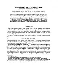
three-level methods do not work for any reasonable time step. For the gradual freezing problem, the present method is three times as fast as the explicit method, 27 times as fast as the best previous three-level method, and 10 times as fast as the iterative methods. In addition, when At is increased above the values given in Table 3, the explicit enthalpy method diverges while the previous three-level methods jump the latent heat peak and give nonsensical results. On the other hand, the present method always gives results within about 10% of the final value, even when At is about l/5 of the total freezing time. This is illustrated in Fig. 1, which shows the percentage discrepancy against At values used for problem 3. 10
-10
h
I
L’~
-
“: \
i’
Q)
R
-20 -
: I :,I I’ I
Y------X
FIG. 1. Plot of discrepancy
35level
+
eq.(3)
vs At for test problem
3.
2. Oscillations Oscillations in the calculated temperature values always occur if sufficiently large time steps are used (Yalamanchili and Chu [ 191; Wood and Lewis [lo]). They tend to happen near the phase-change front where large temperature changes take place. As the time step is reduced, the oscillations rapidly die down. For the problems given, persistent oscillations do not occur if the A.t values of Table 3 are used, except that in problem 2, At has to be reduced to 50 s for the iterative methods [2, 133 and to 20 s for the present method. 3. Complexity of programming and use Programming complexity can be measured by the size of the computer program. For bare-bone programs (one dimension, constant boundary conditions and no input/output statements) the present method and that of ref. [ 131 require 180 FORTRAN77 lines, compared with 130 lines for the explicit enthalpy and previous three-level methods, and 270 lines for the method used in ref. [2]. From the user’s point of view, the iterative methods suffer from the drawback that parameters related to the iterative processes must be chosen. The wrong choice may lead either to incorrect results or to excessive computation times. Unfortunately, the optimal choice varies from problem to problem and there is no a priori way of determining it: a trial-and-error process must be resorted too. Thus, in ref. [ 131, the user must specify the relaxation parameter and the convergence criterion. In ref. [2], the convergence criteria for two different iterative processes must be specified. Noniterative methods (including the present one) do not require the user to make these choices.
A finite-difference scheme for heat conduction with phase change
CONCLUSIONS
The method ofthis paper, which can be called a threelevel enthalpy scheme, combines the best features of enthalpy methods and implicit temperature methods. It is simple to implement, requires no iteration and negligible extra computation per time step, and results in a robust and fast program, resistant to jumping of the latent heat peak. It works equally well for pure cooling, for phase change with abrupt enthalpy change, or for phase change with gradual release of latent heat. For phase-change problems it is two to three times as fast as the best previous method. Although for simplicity of argument the method has been presented in the context of one-dimensional problems and the Lees [S] three-level scheme, extension to two and three dimensions and to other implicit three-level procedures (DuPont et al. [20]) is straightforward. Combination with automatic time step adjustment (Comini et al. [21]) could result in further improvement in speed.
Acknowledgements-The theoretical solution to test problem 1 was found using computer programs written by Dr A. K. Fleming of the Meat Industry Research Institute of New Zealand, to whom thanks are due. The author also thanks Dr A. C. Cleland for his comments.
REFERENCES 1. L. Fox, What are the best numerical methods? In Mouing Boundary Problems in Heat Flow and LX&ion (Edited by J. R. Ockendon and W. R. Hodekins). DD. 21&241. Clarendon Press, Oxford (1975). ” _* 2. R. M. Furzeland, A comparative study of numerical methods for moving boundary problems, J. Inst. Math. Appl. 26,411429 (1980). 3. J. Crank, How to deal with moving boundaries in thermal problems. In Numerical Methods in Heat Transfer (Edited by R. W. Lewis, K. Morgan and 0. C. Zienkiewicz), pp. 177-200. Wiley, New York (1981). 4. V. R. Voller and M. Cross, Use of the enthalpy method in the solution of Stefan problems. In Numerical Methods in Thermal Problems (Edited by R. W. Lewis, J. A. Johnson and W. R. Smith), pp. 91-101. Pineridge Press, Swansea, U.K. (1983). 5. M. Lees, A linear three-level difference scheme for
UN SCHEMA STABLE POUR
2083
quasilinear parabolic equation, Math. Comput. 20, 516 (1976). 6. C. Bonacina and G. Comini, On a numerical method for the solution of the unsteady-state heat conduction equation with temperature dependent parameters. Proc. 13th Int. Cong. Refrig. Vol. 2, p. 329 (1971). 7. G. Comini and R. W. Lewis, A numerical solution of twodimensional problems involving heat and mass transfer, Int. J. Heat Mass Transfer 19, 1387-1392 (1976). 8. J. Succar and K. I. Hayakawa, Parametric analysis for predicting freezing time of infinitely slab-shaped food. J. Food Sci.-49,468277 (1984). _ _ 9. K. Morgan. R. W. Lewis and 0. C. Zienkiewicz. An improvei algorithm for heat conduction problems ‘with phasechange, Int. J. numer. Methods Engng 12,1191-l 195 (1978). 10. W. L. Wood and R. W. Lewis, A comparison of time marching schemes for the transient heat conduction equation, Int. J. numer. Methods Engng 9, 679 (1975). 11. A. C. Cleland, Heat transfer during freezing of foods and predictions of freezing times. Ph.D. thesis, Biotechnology Dept, Massey University, New Zealand (1977). 12. A. C. Cleland and R. L. Earle, Assessment of freezing time prediction methods, J. Food Sci. 49, 10341042 (1984). A numerical method to determine the 13. D. Longworth, temperature distribution around a moving weld pool. In Mooing Boundary Problems in Heat Flow and LXjliision (Edited by J. R. Ockendon and W. R. Hodgkins), pp. 5461. Clarendon Press, Oxford (1975). 14. A. B. Crowley, Numerical solutions of phase change problems, Int. J. Heat Mass Transfer 21,215-219 (1978). 15. C. Bonacina and G. Comini, On the solution of the nonlinear heat conduction equations by numerical methods, Int. J. Heat Mass Transfer 16, 581-589 (1973). 16. A. C. Cleland and R. L. Earle, Prediction of freezing times for foods in rectangular packages, J. Food. Sci. 44, 964970 (1979). 17. H. S. Carslaw and J. C. Jaeger, Conduction of Heat in Solids, 2nd edn. Clarendon Press, Oxford (1959). 18. A. C. Cleland and R. L. Earle, A comparison of analytical
and numerical methods ofpredicting the freezing times of foods, J. Food Sci. 42, 1390-1395 (1977). 19. R. V. S. Yalamanchili and S. C. Chu, Stability and oscillation characteristics of finite-element, finitedifference and weighted-residuals methods for transient two-dimensional heat conduction in solids, Trans. Am. Sot. mech. Engrs, Series C, J. Heat Transfer 85,235 (1973). 20. T. DuPont, G. Fairweather and J. P. Johnson, Three-level Galerkin methods for parabolic equations, SIAM J. numer. Anal. 11, 392410 (1974). 21. G. Comini, S. Del Guidice, R. W. Lewis and 0. C. Zienkiewicz, Finite element solution of non-linear heat conduction problems with special reference to phase change, Int. J. numer. Methods Engng 8, 613-624 (1974).
RAPIDE AUX DIFFERENCES FINIES INCONDITIONNELLEMENT LA CONDUCTION THERMIQUE AVEC CHANGEMENT DE PHASE
R&sum&-Dans la rtsolution numtrique par diffkrences finies des probltmes de conduction thermique avec changement de phase, on peut utiliser des methodes enthalpiques ou des mkthodes de tempirature. Les premikres demandent soit une proddure explicite avec des probl&mes associ&s de convergence, soit une it&ration B chaque pas de temps si des proctdures implicites sont utilistes. Les secondes sont soumises au probltme du saut de chaleur latente qui necessite l’emploi de petits pas de temps pour tviter la sous-estimation des temps de changement de phase. Cette itude suggtire une mkthode simple qui &mine ces problemes et conduit B une proctdure rapide et robuste qui consomme moins de temps de calcul pour le m&me niveau de p&&ion par rapport aux autres schimas aux diffkrences finies.
2084
Q. T. PHAM
EIN SCHNELLES
UND UNEINGESCHRANKT STABILES DIFFERENZENVERFAHREN FUR WARMELEITUNG MIT PHASENANDERUNG
Zusammenfassung-Bei der numerischen Berechnung von Warmeleitproblemen mit Phasentibergang mit Hilfe von Differenzenverfahren kiinnen Enthalpieoder Temperaturverfahren angewandt werden. Die ersteren benijtigen entweder ein explizites Verfahren mit daraus folgenden Konvergenzproblemen oder Iteration in jedem Zeitschritt, wenn implizite Verfahren angewandt werden. Aus den letzteren resultiert das Problem, dag das Maximum der latenten W&me iibersprungen wird, wodurch notwendigerweise kleine Zeitschritte erforderlich sind, urn keine zu kurzen Phasenlnderungszeiten zu berechnen. Dieser Bericht schliigt ein einfaches Verfahren vor, das beide Probleme eliminiert und auf eine schnelle, robuste Prozedur hinauslluft, die weniger Rechenzeit fur dasselbe Genauigkeitsniveau im Vergleich zu anderen Differenzenverfahren benotigt.
6bICTPAR EE3YCJ’IOBHO YCTOH%IBAR KOHEYHO-PA3HOCTHAR CXEMA PEBIEHBS 3AAA9 TEl-IJIOIIPOBO~HOCTM C QA30BbIM I-IEPEXOQOM
JUDl
AIIIIOT~~IIH-~I~HwicneHHoM pememm sana9 rennonpoaoanocrn c $a30BbIMU nepexoaahm r4eronoh.r KOHeYHbIX pa3HOCTek MOryT ACIIOJIb30BaTbCBKBK 3HTEUIbIIHiHbIe, TBK H TeMIICpaTypHbIe MCTOnbI. nepBbIe A3 HUX Tpe6yIoT na60 npllMeHeHkiSi RBHbIXCXeMC IlOCJleilyEOIU&iM PeIIIeHEieM BOII~OCOBCXO~W MOCTH, na60 &iTepaWiii Ha KamnOM BpeMeHHOM LIEWe np&iHCIlOJIb30BaHkiH HellBHbIXMCTOLIOB. TPY~HOCTbIO I,OCJIeLIHAX IIBJIReTCIl CKiFIeK,CBR3aHHbIkCO CKPbITOfiTeIIJIOTOir @33OBOrO IIepeXOna,YTO npHBOJ(HT KHe06XOPMMOCT11 WXO,Ib30BaHH~ MWIbIXBpeMeHHbIXIUEWOB~,I~ ns6emamia HeI'IpenCKa3yeMbIXBpCMe"
@asoaoro
nepexona.
6bICTpykO
HanexHyEo
B pa6ore
npe&Jiox(eH npocToi
npouenypy,KOTOpaa
Tpe6yeT
MeTOn, MeHbUIC
pa3HOCTHbIeCXeMblIlpHTOM
ycTpaHaKxwiii paCYeTHOr0
o6e
TpynHocTA
BpeMeHH,'IeM
XC ypOBHeTOSH0CTH.
A namueti
npyrrte
KOHeSHO-