can be computed in O(m2Alog(m) log(nU)) time, where A is the number of pairs (i, j) with pij = â. .... Following Graham's notation [9], our problem is equivalent to R||Cmax. .... The proof of a similar decomposition theorem can be found in [8].
A Faster Combinatorial Approximation Algorithm for Scheduling Unrelated Parallel Machines Martin Gairing
Burkhard Monien†
∗
Andreas Woclaw
Faculty of Computer Science, Electrical Engineering and Mathematics, University of Paderborn, F¨ urstenallee 11, 33102 Paderborn, Germany. Email: {gairing,bm,wocland}@uni-paderborn.de
∗
A preliminary version of this work appeared in the Proceedings of the 32nd International Colloquium on Automata, Languages and Programming, pp. 828–839, July 2005. This work has been partially supported by the DFG-Sonderforschungsbereich 376 Massive Parallelit¨ at: Algorithmen, Entwurfsmethoden, Anwendungen, by the European Union within the 6th Framework Programme under contract 001907 (DELIS) and by the DFG Research Training Group GK-693 of the Paderborn Institute for Scientific Computation (PaSCo) † Parts of this work were done while the author was visiting Universit` a di Roma La Sapienza at Rome and the University of Texas at Dallas
1
Abstract We consider the problem of scheduling n independent jobs on m unrelated parallel machines without preemption. Job i takes processing time pij on machine j, and the total time used by a machine is the sum of the processing times for the jobs assigned to it. The objective is to minimize makespan. The best known approximation algorithms for this problem compute an optimum fractional solution and then use rounding techniques to get an integral 2-approximation. In this paper we present a combinatorial approximation algorithm that matches this approximation quality. It is much simpler than the previously known algorithms and its running time is better. This is the first time that a combinatorial algorithm always beats the interior point approach for this problem. Our algorithm is a generic minimum cost flow algorithm, without any complex enhancements, tailored to handle unsplittable flow. It pushes unsplittable jobs through a two-layered bipartite generalized network defined by the scheduling problem. In our analysis, we take advantage from addressing the approximation problem directly. In particular, we replace the classical technique of solving the LP-relaxation and rounding afterwards by a completely integral approach. We feel that this approach will be helpful also for other applications.
2
1
Introduction
We consider the scheduling problem where n independent jobs have to be assigned to a set of m unrelated parallel machines without preemption. Processing job i on machine j takes time pij . For each machine j, the total time used by machine j is the sum of processing times pij for the jobs that are assigned to machine j. The makespan of a schedule is the maximum total time used by any machine. The objective is to find a schedule (assignment) that minimizes makespan. This problem has many applications. Typically, they arise in the area of scheduling multiprocessor computers and industrial manufacturing systems (see e.g. [18, 29]).
1.1
Related Work
There is a large amount of literature on scheduling independent jobs on parallel machines (a collection of several approximation algorithms can be found in [10]). A good deal of these publications concentrate on scheduling jobs on unrelated machines. Horowitz and Sahni [11] presented a (non-polynomial) dynamic programming algorithm to compute a schedule with minimum makespan. Lenstra et al. [17] proved that unless P = N P, there is no polynomialtime approximation algorithm for the optimum schedule with approximation factor less than 23 . They also presented a polynomial-time 2-approximation algorithm. This algorithm computes an optimal fractional solution and then uses rounding to obtain a schedule for the discrete problem with approximation factor 2. Shmoys and Tardos [24] generalized this technique to obtain the same approximation factor for the generalized assignment problem. They also generalized the rounding technique to hold for any fractional solution. Recently, Shchepin and Vakhania [23] 1 . introduced a new rounding technique which yields the improved approximation factor of 2 − m
The fractional unrelated scheduling problem can also be formulated as a generalized maximum flow problem, where the network is defined by the scheduling problem and the capacity of some edges, that corresponds to the makespan, is minimized. This generalized maximum flow problem is a special case of linear programming. Using techniques of Kapoor and Vaidya [14] and by exploiting the special structure of the problem, an optimum fractional solution can be found with the interior point algorithm of Vaidya [28] in time O(|E|1.5 |V |2 log(U )), where U denotes the maximal pij . In contrast to the linear programming methods, the aforementioned generalized maximum flow problem can also be solved with a purely combinatorial approach. Here, the makespan minimization is done by binary search. Computing generalized flows has a rich history, going back to Dantzig [2]. The first combinatorial algorithms for the generalized maximum flow problem were exponential time augmenting path algorithms by Jewell [13] and Onaga [19]. 3
Truemper [27] showed that the generalized maximum flow problem and the minimum cost flow problem are closely related. More specifically, he transformed a generalized maximum flow problem into some minimum cost flow problem by setting the cost of an edge to be the logarithm of the gain from the generalized maximum flow problem. Goldberg et al. [6] designed the first polynomial-time combinatorial algorithms for the generalized maximum flow problem. Their algorithms were further refined and improved by Goldfarb, Jin and Orlin [7] and later by Radzik [22]. Radzik’s algorithm is so far the fastest combinatorial algorithm with a running time of O(|E| |V |(|E| + |V | log |V |) log U ). In order to minimize makespan, this algorithm has to be called at most O(log(nU )) times. There exist fast fully polynomial-time approximation schemes for computing a fractional solution [4, 12, 20, 21, 26]. Using the rounding technique from [24], this leads to a (2 + ε)approximation for the discrete problem. The approximation schemes can be divided into those that approximate generalized maximum flows [4, 21, 26] and those that directly address the scheduling problem [12, 20]. Unrelated machine scheduling is a very important problem and many heuristics and exact methods have been proposed. Techniques used here range from combinatorial approaches with partial enumeration to integer programming with branch-and-bound and cutting planes. For a selection we refer to [18, 25, 29] and references therein. Finding a discrete solution for the unrelated scheduling problem can be formulated as an unsplittable generalized maximum flow problem. Several authors [3, 15, 16] have studied the unsplittable flow problem for usual flow networks. Kleinberg [15] formulated the problem of finding a solution with minimum makespan for the restricted scheduling problem as an unsplittable flow problem. Here the restricted scheduling problem is a special case of our problem, in which each job i has some weight wi , each machine j has some speed sj and pij =
wi sj
or pij = ∞ holds for all i, j. Gairing et al. [5] exploited the special structure of
the network, gave a 2-approximation algorithm for the restricted scheduling problem based on preflow-push techniques and also an algorithm for computing a Nash equilibrium for the restricted scheduling problem on identical machines.
1.2
Contribution
The algorithm presented in this paper computes an assignment for the unrelated scheduling problem with makespan at most twice the optimum. We prove that a 2-approximative schedule can be computed in O(m2 A log(m) log(nU )) time, where A is the number of pairs (i, j) with pij 6= ∞. This is better than the previously known best time bounds of Vaidya’s [28] and
4
Radzik’s [22] algorithms. In particular, this is the first time that a combinatorial algorithm always beats the interior point approach for this problem. An essential element of our approximation algorithm is the procedure Unsplittable-BlockingFlow from [5]. This procedure was designed to solve the unsplittable maximum flow problem in a bipartite network, which is defined by the restricted scheduling problem. In this paper the connection to flow is more tenuous. We solve an unsplittable flow problem in a generalized bipartite network, which is defined by the unrelated scheduling problem. The generalized flow problem can be transformed to a minimum cost flow problem. Our algorithm uses the primaldual approach combined with a gain scaling technique to obtain a polynomial running time. To compute a flow among the edges with zero reduced cost it uses the procedure UnsplittableBlocking-Flow from [5] in the inner loop. Given some candidate value for the makespan, our algorithm finds an approximate solution for the generalized flow problem in the two-layered bipartite network. Throughout execution the algorithm always maintains an integral assignment of jobs to machines. Each assignment defines a partition of the machines into underloaded, medium loaded and overloaded machines. Our overloaded machines are heavily overloaded, that is, their load is at least twice as large as the candidate makespan. The main idea of our algorithm is to utilize the existence of overloaded machines in conjunction with the fact that we are looking for an approximate integral solution. We use this idea twice. On the one hand this allows us to show an improved lower bound on the makespan of an optimum schedule and thus to overcome the (1 + ε) error usually induced by the gain scaling technique. On the other hand this is also used to reduce the number of outer loops to O(m log m), which is the main reason for the substantial running time improvement. Our algorithm is a generic minimum cost flow algorithm without any complex enhancements for generalized flow computation. Overloaded and underloaded machines are treated as sources and sinks, respectively. The height of a node is its minimum distance to a sink. In our algorithm the admissible network, used for the unsplittable maximum flow computation, consists only of edges and nodes which are on shortest paths from overloaded machines with minimum height to underloaded machines. This modification to the primal-dual approach is important to show the improved lower bound on the makespan of an optimum schedule. Our algorithm is simpler and faster than the previously known algorithms. For the unrelated scheduling problem we have replaced the classical technique, i.e., computing first a fractional solution and rounding afterwards, by a completely integral approach. Our algorithm takes advantage from addressing the approximation problem directly. In particular, this allows us to benefit from an unfavorable preliminary assignment. We feel that this might be helpful also in other applications. 5
Identifying the connection to flow might be the key for obtaining combinatorial (approximation) algorithms for problems for which solving the LP-relaxation and rounding is currently the (only) alternative. Our techniques and results do not improve upon the approximation factor for the unrelated scheduling problem, however, we expect improvements for other hard problems.
1.3
Comparison of Running Times
We compare the running time of our algorithm with the so far fastest algorithms of Vaidya [28] and Radzik [22]. Both of the former approaches have been designed to solve the fractional generalized maximum flow problem on a graph with node set V and edge set E. Rounding the fractional solution yields the 2-approximation. Technique and running time for computing a 2-approximative schedule: • Interior Point approach for generalized flow problem and rounding [28] O(|E|1.5 |V |2 log(U )) • Combinatorial algorithm for generalized flow problem and rounding [22] O(|E| |V |(|E| + |V | log |V |) log U log(nU )) • The integral approach presented in this paper O(m2 A log(m) log(nU )) To compare these bounds, note that in our bipartite network A = |E| = O(nm) and |V | = n+m. Our algorithm is linear in A. It clearly outperforms the previous algorithms if n + m = 0.5
(n+m) o(A). In the case A = Θ(n + m) our algorithm is better by a factor of Ω( log(n) log(m) ) than
Vaidya’s algorithm and by a factor of Ω(log U ) faster than Radzik’s algorithm. This is the first time that a combinatorial algorithm always beats the interior point approach for this problem. The heuristics [18, 25, 29] consider instances where A = Θ(nm). In this case our algorithm outperforms both former approaches by a factor almost linear in n. The (1 + ε)-approximation algorithms for the generalized maximum flow problem in [4, 21, e e notation hides a 26] have all running time O(log ε−1 |E|(|E| + |V | log log U )), where the O() factor polylogarithmic in |V |. Again, an extra factor of O(log(nU )) is needed for the makespan minimization. This running time is not always better than ours. The fastest approximation scheme that directly addresses the scheduling problem is due to Jansen and Porkolab [12] and 6
has a running time of O(ε−2 (log ε−1 )mn min{m, n log m} log m). Clearly, for constant � this algorithm is faster than our algorithm. However, for � in the order of
1 m
and log(U ) = O(n)
their running times become comparable. Recall, that the (1 + ε)-approximation algorithms for the generalized maximum flow problem plus rounding yield a (2 + ε)-approximation for the unrelated scheduling problem.
2
Notation
2.1
The scheduling problem
We consider the problem of scheduling a set J of n independent jobs on a set M of m machines. The processing time of job i on machine j is denoted by pij . Define the n × m matrix of processing times P in the natural way. Throughout the paper we assume that pij is either an integer or ∞ for all i ∈ J and j ∈ M . Define U = maxi∈J,j∈M {pij 6= ∞}. Furthermore, define A as the number of pairs (i, j) with pij 6= ∞. An assignment of jobs to machines is denoted by a function α : J 7→ M . We denote α(i) = j if job i is assigned to machine j. For any assignment α, the load δj on machine j for a matrix of processing times P is the sum of processing times for the jobs that are assigned to machine j, thus X
δj (P, α) =
pij .
i∈J,α(i)=j
We omit P in the notation of δj if P is clear from the context. Define the makespan of an assignment α for a processing time matrix P, denoted Cost(P, α), as the maximum load on a machine, hence Cost(P, α) = max δj (α). j∈M
Associated with a matrix of processing times P is the optimum makespan, which is the least possible makespan of an assignment α, that is OPT(P) = min Cost(P, α). α
Following Graham’s notation [9], our problem is equivalent to R| |Cmax .
2.2
Generalized Maximum Flows and Minimum Cost Flows
The generalized maximum flow problem is a generalization of the maximum flow problem, where each edge (i, j) has some gain factor µij . If fij units of flow are sent from node i to node j 7
along edge (i, j), then µij fij units arrive at j. More specifically, let G = (V, E) be a directed graph of the generalized flow problem, µ : E 7→ R+ a gain function, and s and t source and sink node, respectively. Furthermore, there is a capacity function u : E 7→ R+ on the edges. A generalized flow f : E 7→ R is a function on the edges that satisfies the capacity constraints, the antisymmetry constraints fij = −µji · fji on all edges (i, j) ∈ E, and the conservation P P constraints (j,i)∈E µji fji − (i,j)∈E fij = 0 on all nodes i ∈ V \ {s, t}. Given a generalized flow f , the residual capacity is a function uf : E 7→ R+ defined by uf (i, j) = u(i, j) − fij on all edges (i, j) ∈ E. The residual network with respect to some generalized flow f is the network Gf = (V, Ef ) where Ef = {(i, j) ∈ E : uf (i, j) > 0} The value of the flow f is defined as the amount of flow into the sink. Among all generalized flows of maximum value, the goal is to find one that minimizes the flow out of the source. The fractional version of the scheduling problem can be converted into a generalized maximum flow problem [20]. In order to check whether a fractional schedule of length w exists, one can construct a bipartite graph with nodes representing jobs and machines and introduce an edge from machine node i to job node j with gain 1/pij . There is a source which is connected to all the machine nodes with edges of unit gain and capacity w, and the job nodes are connected to a sink with edges of unit gain and unit capacity. A generalized flow in this network that results in an excess of n at the sink corresponds to a solution of the fractional scheduling problem. If the maximum excess that can be generated at the sink is below n, then the fractional scheduling problem is infeasible, i.e., the current value of w is too small. Truemper [27] established a relationship between the generalized maximum flow problem and the minimum cost flow problem. In his construction, he defined the cost for each edge in the minimum cost flow problem as the logarithm of the gain in the generalized maximum flow problem. In order to transform the generalized maximum flow problem to a minimum cost flow problem with integral edge costs, a gain rounding technique can be used (see e.g. [26]). Gains are rounded down to integer powers of some base b > 1. The rounded gain of each edge (i, j) is defined as γij = bcij where cij = blogb µij c. Antisymmetry is maintained by setting γij = 1/γji and cij = −cji . The cost of edge (i, j) in the resulting minimum cost flow problem equals cij . Using a potential function π : V 7→ R+ , the reduced costs cπij of an edge (i, j) are defined as cπij = cij − π(i) + π(j) (see [1]). The Primal-Dual approach [1] for minimum cost flows can be used to compute a generalized maximum flow (see e.g. [26]). The Primal-Dual approach preserves the reduced cost optimality condition, i.e., cπij ≥ 0 for each edge (i, j) in the residual network. Because of the rounding, an optimum solution of the minimum cost flow problem gives only a (1 + �)-approximation of the generalized (fractional) maximum flow problem. Because of the special structure of the problem and in contrast to [26], it suffices to choose b = 1 + ε to get this (1 + �)-approximation. Using techniques from [24], the fractional solution can be 8
transformed to an integral solution. This approach leads to a (2 + �)-approximation algorithm for the scheduling problem.
2.3
Our model
We also formulate the scheduling problem as a generalized maximum flow problem. However, we use a different construction as in [20]. We construct a bipartite graph with nodes representing jobs and machines. There is an edge from job node i to machine node j with unit capacity and gain µij = pij if pij ≤ w. The parameter w will be determined by binary search. Each job node i has supply 1. A generalized flow f is a solution to the fractional version of the scheduling problem, if in f all supplies are sent to the machines. In this case, we call f a feasible flow. A generalized flow in such a network creates excess on the machine nodes. An excess on machine j corresponds to the load on machine j. Define δj (P, f ) as the load on machine j under the generalized flow f with gains defined by P. If we require that the supply of each job is sent to exactly one machine, then we get an integral solution to the scheduling problem. In this case, we call f a generalized unsplittable flow and f corresponds to an assignment α, i.e., assigning job i to machine j corresponds to sending one unit of flow along edge (i, j). By the construction of our bipartite graph, the assignment α has the property that each job i is assigned to a machine j where pij ≤ w. In the following we call such an assignment w-feasible. We sometimes omit the term w-feasible, if it is clear from the context. We are interested in finding a generalized unsplittable flow f such that the maximum excess over all machines is at most 2w. This is not always possible, however, if we can’t find such a flow, we can still derive the lower bound OPT(P) ≥ w + 1. Following the construction from Section 2.2, we formulate this generalized maximum unsplittable flow problem as a minimum cost flow problem. For the gain rounding, we choose b = (1 +
1 m ).
If (i, j) is an edge from job node i to machine node j then the cost cij and the
rounded gain γij is defined by and γij = bcij .
cij = blogb (pij )c, For any path W , we define γ(W ) =
Q
(i,j)∈W
γij . In the same way we define γ(K) for some
cycle K. In the following, denote C = (cij ) and Γ = (γij ). In order to solve the minimum cost flow problem we use the well known Primal-Dual approach [1]. For a a positive integer w, a w-feasible assignment α and a matrix of processing times P, we now define the residual network Gα (w) (Definition 2.1) and we partition the machines, with respect to their loads, into three subsets (Definition 2.2).
9
Definition 2.1 Let w ∈ N and α be a w-feasible assignment. We define a directed bipartite graph Gα (w) = (V, Eα (w)) where V = M ∪ J and each machine is represented by a node in M , whereas each job defines a node in J. Furthermore, Eα = Eα1 ∪ Eα2 with Eα1 = {(j, i) : j ∈ M, i ∈ J, α(i) = j, pij ≤ w} , and Eα2 = {(i, j) : j ∈ M, i ∈ J, α(i) 6= j, pij ≤ w} . Definition 2.2 Let w ∈ N and α be an w-feasible assignment. We partition the set of machines M into three subsets: M − (α) = {j : δj (P, α) ≤ w} M 0 (α) = {j : w + 1 ≤ δj (P, α) ≤ 2w} M + (α) = {j : δj (P, α) ≥ 2w + 1} In our setting, at each time, nodes from M − can be interpreted as sink nodes, whereas nodes from M + as source nodes. We now give a lemma that generalizes the path decomposition theorem to generalized flows. The proof of a similar decomposition theorem can be found in [8]. A fractional generalized flow on a path is defined as a flow that fulfills the flow conservation constraints on the inner nodes. Similarly, a generalized flow on a cycle fulfills the flow conservation constraints on all nodes in the cycle except one. Lemma 2.1 (Decomposition theorem) Let f and g be two generalized feasible flows in G = (J ∪ M, E). Then g equals f plus fractional flow: (a) on some directed cycles in Gf , and (b) on some directed paths in Gf with end points in M and with the additional property that no end point of some path is also the starting point of some other path. ˜ = {(i, j); hij > 0, (i, j) ∈ Ef } ∪ {(j, i); hij < 0, (i, j) ∈ Ef }. We Let h = g − f . Set E ˜ ⊂ Ef . Let gij and fij be the flows on edge (i, j) in Gg and Gf , respectively, show first that E Proof:
and u(i, j) its capacity. Then gij > fij
⇒ fij < u(i, j) ⇒ (i, j) ∈ Ef , and
gij < fij
⇒ fij > 0 ⇒ (j, i) ∈ Ef .
10
˜ and u ˜ Since f and g are both feasible Let u ˜(i, j) = hij if (i, j) ∈ E, ˜(i, j) = −hij if (j, i) ∈ E. they both send all supply from the job nodes J to the machine nodes M . It follows that for each job node i ∈ J, X
hij −
˜ (i,j)∈E
X
µji · hji = 0,
˜ (j,i)∈E
and thus h fulfills the flow conservation constraints on all job nodes J. ˜ If there exists a cycle in the graph induced by E, ˜ We will now decompose the flow in E. let us choose some node u ∈ M on the cycle and determine the maximal flow x which can be pushed from u along this cycle without conflicts to the capacity constraints. Subtract this flow ˜ By subtracting this flow we maintain the flow conservation constraints on from the flow in E. ˜ Let us all job nodes J. Since x was chosen to be maximal, at least one edge is deleted from E. ˜ Afterwards, E ˜ defines proceed this way as long as there are cycles in the graph induced by E. a directed acyclic graph. Now choose a path connecting a node u of in-degree 0 to a node v of out-degree 0, determine ˜ Note that at least one the maximum allowed flow on this path and delete this flow from E. ˜ Furthermore, by the flow conservation constraint, any job node i ∈ J edge is deleted from E. with out-degree 0 has also in-degree 0. This implies v ∈ M . Let us proceed this way until there ˜ The way the paths are chosen guarantees that no end point of some path is are no edges in E. also a starting point of some other path.
2.4
Unsplittable Blocking Flows
Our approximation algorithm will make use of the algorithm Unsplittable-Blocking-Flow introduced in [5]. Unsplittable-Blocking-Flow was designed for a restricted scheduling problem on identical machines. Here, each job i has some weight wi and is only allowed to use a subset Ai of the machines. This is a special case of the unrelated scheduling problem considered in this paper, where pij = wi if j ∈ Ai and pij = ∞ otherwise. Given an integer w and a w-feasible assignment α, Unsplittable-Blocking-Flow(α, w) computes a w-feasible assignment β, where there is no path from M + (β) to M − (β) in Gβ (w). In the following we present a version of algorithm Unsplittable-Blocking-Flow adapted to the setting of this paper, i.e., it runs on processing times pij and pushes jobs only along edges from some subgraph G0α (w) of graph Gα (w). This subgraph G0α (w) has the property that each job node has exactly one incoming edge (from the machine to which it is assigned by α) and at least one outgoing edge.We define G0α (w) in Section 3.1. We will also call this modified algorithm Unsplittable-Blocking-Flow. These adaptations do not influence the correctness
11
and the running time of algorithm Unsplittable-Blocking-Flow. Our adapted algorithm is depicted in Figure 1. Unsplittable-Blocking-Flow reassigns jobs so that the loads of machines from M − never decrease, the loads of machines from M + never increase, and machines from M 0 stay in M 0 . It receives as input an assignment α, a graph G0α (w) = (Eα0 , Vα0 ), a matrix of processing times P and positive integer w. When Unsplittable-Blocking-Flow terminates we have computed a new assignment β, having the property, that in G0β (w) there is no path from M + (β) to M − (β). Unsplittable-Blocking-Flow is controlled by a height function h : V 7→ N0 with h(j) = distG0α (j, M − ), ∀j ∈ Vα0 . Here the distance is defined as the number of edges. Observe, that h induces a levelgraph on G0α (w). We call an edge (u, v) ∈ G0α (w) admissible with respect to the height function h (or just admissible, if h is clear from the context), if h(u) = h(v) + 1. In an admissible path all edges are admissible. For each node j ∈ V with 0 < h(j) < ∞, let S(j) be the set of nodes to which j has an admissible edge, i.e. � S(j) = i ∈ V : (j, i) ∈ Eα0 and h(j) = h(i) + 1 . Let s(j) be the first node on list S(j).
The following two definitions are important for
Unsplittable-Blocking-Flow. Definition 2.3 A machine j ∈ V is called helpful, with respect to some integer w and some w-feasible assignment α, if h(j) < ∞ and δj (α) ≥ w + 1 + ps(j),j . Observe, that a machine in j ∈ M + is always helpful since only jobs i with pij ≤ w are assigned to it. Definition 2.4 A helpful path is a sequence v0 , . . . , vr , where s(vi ) = vi+1 for all 0 ≤ i ≤ r −1, v2i ∈ M for all 0 ≤ i ≤ r/2 and v2i+1 ∈ J for all 0 ≤ i < r/2 such that: (1) v0 is a helpful machine of minimum height, (2) (vi , vi+1 ) ∈ Eα0 and h(vi ) = h(vi+1 ) + 1, (3) w + 1 ≤ δv2i + ps(v2i−2 ),v2i − ps(v2i ),v2i ≤ 2w for all 0 < i < r/2, (4) δvr + ps(vr−2 ),vr ≤ 2w. If we reassign jobs according to a helpful path, then • by (1) the load on machine v0 decreases but not below w + 1; • by (2) we reassign jobs only according to admissible edges; 12
• by (3) all machines v2i with 0 < i < r/2 stay in M 0 ; • by (4) the load on machine vr increases but not above 2w. With a similar argumentation as in [5, Lemma 4.1] we can show that each helpful machine of minimum height defines a helpful path. Unsplittable-Blocking-Flow(α, G0α (w), P, w) Input: assignment α, graph G0α (w) matrix of processing times P positive integer w Output: assignment β 1:
compute h;
2:
while M − 6= ∅ and ∃j ∈ M + with h(j) < ∞ do
3:
d ← minj∈M + (h(j));
4:
while ∃ admissible path from j ∈ M + with h(j) = d to M − in the graph G0α (w) do
5:
choose some helpful machine v ∈ M of minimum height;
6:
push jobs along some helpful path defined by v;
7:
update α, G0α (w), M + , M − ;
8:
end while
9:
recompute h;
10:
end while
11:
return α; Figure 1: Unsplittable-Blocking-Flow Unsplittable-Blocking-Flow terminates, when M − = ∅ or when h(j) = ∞ for all
machines j ∈ M + . The algorithm works in phases. Before the first phase starts, the height function h is computed as the distance in G0α of each node to a node in M − . While computing h we also collect the set of admissible edges with respect to h. In each phase, first the minimum height d = h(j) of a machine j ∈ M + is computed. Inside a phase we do not update the height function h, but we successively choose a helpful machine v of minimum height and we push jobs along the helpful path induced by v and adjust the assignment accordingly. Each job push is a reassignment of the corresponding job. In order to update G0α we have to change the direction of two edges for each job push. The newly created edges are not admissible with respect to h. To update M + and M − is suffices to check the load on the first and the last machine of the helpful path. The phase ends, when no further admissible path from a machine j ∈ M + with h(j) = d to some machine in M − exists in the levelgraph defined by the admissible edges with respect to the height function h. Before the new phase starts, we recompute h and we check 13
whether we have to start a new phase or not. We show in [5] that there are at most m phases and that the running time of each phase is dictated by the computation of the height function, which can be done by breath-first-search in time O(A). Lemma 2.2 and Theorem 2.3 are derived from [5] and state properties of algorithm Unsplittable-Blocking-Flow that are used in the discussion of our approximation algorithm. Their proofs are direct generalizations of the corresponding proofs in [5]. For details on the analysis we refer to [5]. Lemma 2.2 ([5, Lemma 4.2]) Let β be the assignment computed by UnsplittableBlocking-Flow(α, G0α (w), P, w). Then (a) j ∈ M − (α) ⇒ δj (P, β) ≥ δj (P, α) (b) j ∈ M 0 (α) ⇒ w + 1 ≤ δj (P, β) ≤ 2w (c) j ∈ M + (α) ⇒ δj (P, β) ≤ δj (P, α). Lemma 2.2 ensures that the loads of machines from M − never decrease, the loads of machines from M + never increase, and machines from M 0 stay in M 0 . Let G0α (w) be the subgraph of Gα (w). Let β be the assignment computed by UnsplittableBlocking-Flow(α, G0α (w), P, w). In this call jobs are reassigned by pushing them through edges of G0α (w). We define G0β (w) as the graph that results from G0α (w) after this reassignments. Theorem 2.3 ([5, Lemma 4.4/Theorem 4.5])
Algorithm Unsplittable-Blocking-
Flow(α, G0α (w), P, w) takes time O(mA) and computes an assignment β, having the property, that there is no path from M + (β) to M − (β) in G0β (w).
3
Approximation Algorithm
We now present our approximation algorithm, Unsplittable-Truemper, which will be used to compute an assignment α where Cost(P, α) ≤ 2·OPT(P). We always maintain an unsplittable flow, i.e., an integral solution. We loose a factor of 2 by allowing some gap for the machine loads. The special structure of our algorithm allows us to compensate the error, introduced by the gain scaling technique, by a better lower bound on OPT(P). We stop the computation as soon as we get this better lower bound. This improves also the running time. 14
3.1
Algorithm Unsplittable-Truemper
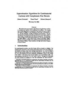
We formulate the scheduling problem as a generalized maximum unsplittable flow problem with rounded gain factors as described in Section 2.2. In order to solve this generalized unsplittable flow problem we use the Primal-Dual approach for computing a minimum cost flow [1]. Our algorithm maintains the reduced cost optimality condition. In our setting this means that it does not create negative cost cycles in the residual network. In order to achieve this, Unsplittable-Truemper iteratively computes a shortest path graph G0α (w), which we define below, and uses Unsplittable-Blocking-Flow to compute a blocking flow on this shortest path graph. While the costs in Unsplittable-Truemper refer to the rounded processing times, it operates on the original processing times. It is important to note, that both the costs as well as the original processing times are integer. Because of Theorem 2.3, there is no path from a machine from M + to a machine from M − in G0α (w) after termination of UnsplittableBlocking-Flow. We stop this procedure, when we can either derive a good lower bound on OPT(P) (see Theorem 3.3) or we found an assignment α with M + = ∅. Unsplittable-Truemper(α, P, C, w) Input: assignment α where each job i is assigned to a machine from B(i) matrix of processing times P and matrix of edge costs C positive integer w Output: assignment β // Gα (w) is the graph corresponding to α and w. 1:
π ← 0;
2:
while ∃j ∈ M + with a path to k ∈ M − in Gα (w) and ∀u ∈ M + : π(u) < logb (m) do
3:
compute shortest path distances d(·) from all nodes to the set of sinks M − in Gα (w) with respect to the reduced costs cπij ;
4:
π ← π + d;
5:
+ as the set of machines from M + with minimum distance to a node in M − define Mmin
with respect to the costs cij ; 6:
define G0α (w) as the admissible graph consisting only of edges on shortest paths from + Mmin to M − in Gα (w);
7:
β ← Unsplittable-Blocking-Flow(α, G0α (w), P, w);
8:
α ← β;
9:
end while
10:
return α; Figure 2: Unsplittable-Truemper
15
We now describe our algorithm in more detail. Unsplittable-Truemper starts with an assignment α. In α, each job i ∈ J is assigned to some machine j ∈ B(i), where its processing time is minimum, i.e., B(i) = {j ∈ M : pij ≤ pik , ∀k ∈ M }. Arc capacities are given by P whereas edge costs are given by C (as defined in Section 2). Furthermore, UnsplittableTruemper gets as input an integer w, which is large enough so that α is w-feasible; that is, w ≥ maxi∈[n] minj∈[m] {pij }. Assignment α and integer w define a graph Gα (w) as in Definition 2.1, and a partition of the machines as in Definition 2.2. At all times, UnsplittableTruemper maintains a total assignment, that is all jobs are always assigned to some machine. If a job gets unassigned from a machine, it is immediately assigned to some other machine. Our algorithm iteratively computes shortest path distances d(u) from each node u to the set of sinks M − , with respect to the reduced costs cπij . Then π is updated, such that all edges on shortest paths have zero reduced costs. For each node u ∈ M , π(u) never decreases. After the update of π, π(u) holds the minimum distance from u to M − for each node u with respect to + the costs cij . We define Mmin as the set of machines from M + with minimum distance to a node + consists of all machines u ∈ M + where in M − with respect to the costs cij . Note, that Mmin
π(u) is minimum. G0α (w) is then defined as the admissible graph, consisting only of edges on + to M − in Gα (w). We will see in Section 3.2 that this is essential for shortest paths from Mmin
our algorithm. Note, that G0α (w) consists only of edges with zero reduced costs. Afterwards, Unsplittable-Blocking-Flow is applied to the admissible graph G0α (w). It reassigns jobs from the admissible graph, such that after Unsplittable-Blocking-Flow returns, there is + no longer a path from a machine in Mmin to a machine in M − in the admissible graph G0α (w).
Therefore, min{π(u); u ∈ M + } increases in the next iteration of the while loop. The residual network Gα (w) is then updated accordingly. The while-loop terminates when there exists no machine from M + with a path to a machine from M − in Gα (w) or there exists a machine u ∈ M + with π(u) ≥ logb (m).
3.2
Analysis
We now analyze the behavior of our algorithm. The main result in this section is Theorem 3.3. A call of Unsplittable-Truemper(α, P, C, w) terminates if M + (α) = ∅. In this case, we know that Cost(P, α) ≤ 2w. We will see, that we can take also some advantage from an assignment α which is still unfavorable, i.e., for which M + (α) 6= ∅ holds. The reduced cost optimality condition cπij ≥ 0 holds for all (i, j) ∈ Eα (w) during the whole computation. It implies γ(K) ≥ 1 for each cycle K in Gα (w). This property does not necessarily hold for every path. Lemma 3.1 is of crucial importance in our analysis. It shows that γ(W ) ≥ 1 holds for every path W connecting some node from M + (α) to any other node from M in Gα (w). 16
For proving this result, we need that G0α (w) was defined only by shortest paths from nodes in + Mmin to nodes in M − .
Lemma 3.1 Unsplittable-Truemper Gα (w) from any machine in Proof:
M+
maintains the property, that for each path W in
to any other machine in M , we have γ(W ) ≥ 1.
We show that the claim is an invariant of the algorithm. The property holds at the
beginning, since each job i is assigned to a machine j ∈ B(i). Assume the claim holds at some time of the execution of Unsplittable-Truemper. We will show that after the next reassignment the claim still holds. Our algorithm only reassigns jobs on shortest paths from + Mmin to M − . For any two nodes u, v ∈ V denote Wu,v as a path from u to v in Gα (w) where
γ(Wu,v ) is minimum. If no such path exists, define γ(Wu,v ) = ∞. Let j be any machine from + Mmin and let i be any job on a shortest path from j to M − . We may assume that i gets
reassigned from some machine u to some machine v. Define y = γ(Wu,v ) and x = γ(Wj,u ). Note, that this implies γ(Wj,v ) = xy. Let k be any machine from M + and consider any path from k to some other machine h ∈ M . Since j has minimum distance to M − , we know + that γ(Wk,u ) ≥ x and γ(Wk,v ) ≥ xy, otherwise j 6∈ Mmin . By reassigning i, γ(Wu,v ) can
not decrease. Only γ(Wv,u ) on the path from v to u might decrease. If γ(Wv,u ) does not decrease, the claim follows immediately. So assume γ(Wv,u ) decreased. However, then γ(Wv,u ) is defined by the new path (v, i, u) and thus γ(Wv,u ) = y1 . Now consider path Wk,h . If Wk,h does not go through (v, i, u), then γ(Wk,h ) did not change. However, if Wk,h uses (v, i, u), then γ(Wk,h ) = γ(Wk,v ) · γ(Wv,u ) · γ(Wu,h ) ≥ x · γ(Wu,h ). Since j has a path to u with Wj,u = x and γ(Wj,h ) ≥ 1, it follows that γ(Wu,h ) ≥ x1 . Thus, Wk,h ≥ 1. This completes the proof of the lemma. The following lemma will be used to derive a lower bound on OPT(P). Lemma 3.2 Let (G, Γ) denote a generalized maximum unsplittable flow problem defined by network G and matrix of processing times Γ. Let f be a generalized feasible unsplittable flow in (G, Γ), and let s, t ∈ R+ . Suppose ∀u ∈ M : δu (Γ, f ) ≥ s, and ∃ˆ u ∈ M : δuˆ (Γ, f ) ≥ s + t, and for each cycle K in Gf , γ(K) ≥ 1. If on every path W in Gf from u ˆ to any other machine u ∈ M , γ(W ) ≥ 1, then OPT(Γ) ≥ s +
t m.
Let f ∗ be an optimum generalized fractional flow in (G, Γ) and define f˜ = f ∗ − f . Consider the cycle/path decomposition of f˜ according to Lemma 2.1. Recall, that in this Proof:
cycle/path decomposition no end node of some path is also a starting node of some other path. Note, that γ(K) ≥ 1 for any cycle K. This implies that pushing flow along any cycle K does 17
not decrease the load on any of its machines. By pushing flow along a path W , only the load of the starting node of W can be decreased. The load on the inner nodes of W does not change and the last node receives load. Since γ(W ) ≥ 1, the increase in the load of the end node is not smaller than the decrease of the load of the starting node. Together with the assumption that δu (Γ, f ) ≥ s for all u ∈ M and δuˆ (Γ, f ) ≥ s + t, this implies that OPT(Γ) ≥ s +
t m.
Theorem 3.3 Algorithm Unsplittable-Truemper takes time O(m2 A log(m)). Furthermore, if Unsplittable-Truemper(α, P, C, w) terminates with M + 6= ∅ then OPT(P) ≥ w + 1. Proof:
We will first show, that Unsplittable-Truemper
terminates after at most
O(m log(m)) iterations of the while loop. Now consider one iteration. Recall, that π(u) for each node u ∈ M never decreases. Unsplittable-Blocking-Flow terminates if and only if + there is no path from Mmin to M − in the residual network. According to Lemma 2.2, it does + not add nodes to M + . Afterwards, either Mmin = ∅ or the distance d(u) with respect to the + + reduced costs cπij from any node u ∈ Mmin to a sink is at least 1. If Mmin = ∅ then in the next + is defined by a new set of nodes from M + with larger potential π. In each case, iteration Mmin + increases at least by one in each iteration. The algorithm terminates if there π(u) for u ∈ Mmin
exists a node u ∈ M + with π(u) ≥ logb (m). Note, that logb (m) =
log2 (m) log2 (m) = = O(m · log(m)). log2 (b) log2 (1 + 1/m)
Thus, at most O(m log(m)) iterations of the while loop are possible. The running time of one iteration of the while loop is dominated by the running time of Unsplittable-Blocking-Flow. Due to Theorem 2.3, this takes time O(mA). Thus, the total running time of UnsplittableTruemper is O(m2 A log(m)). This completes the proof of the running time. We now show the lower bound on OPT(P).
Let β be the assignment, computed by
Unsplittable-Truemper(α, P, C, w). In the construction of our graph Gα (w) we only have edges for processing times not greater than w. Thus, we will not assign a job i to a machine j with pij ≥ w + 1. If in an optimum assignment a job i is assigned to a machine j with pij ≥ w + 1 then OPT(P) ≥ w + 1 follows immediately. So, in the following we can assume, that in an optimum assignment, each job i ∈ J is only assigned to a machine j ∈ M with pij ≤ w. Note, that Unsplittable-Truemper maintains the reduced cost optimality condition for rounded gains Γ. Since for each edge (i, j) we have γij ≤ pij ≤ bγij , it follows that δu (P, β) ≤ b · δu (Γ, β) for all u ∈ M . Since Unsplittable-Truemper terminated, there is either no longer a path from M + to M − in the residual graph Gβ (w) or there exists a machine u ∈ M + with π(u) ≥ logb (m). 18
Case I: 6 ∃ path from M + to M − in Gβ (w). f as the set of machines still reachable from M + in Gβ (w). The load of jobs assigned Define M f can not be distributed to the other machines. For each machine j ∈ M f, to a machine from M we have δj (P, β) ≥ w + 1 and therefore δj (Γ, β) ≥
1 b (w
+ 1). Furthermore, since M + 6= ∅,
there exists a machine v with δv (P, β) ≥ 2w + 1. This implies δv (Γ, β) ≥
1 b (2w
+ 1). Since
Unsplittable-Truemper maintains the reduced cost optimality condition for the rounded gains, we have γ(K) ≥ 1 for any cycle K in Gβ (w). By Lemma 3.1, γ(W ) ≥ 1 for each path from any machine in M + to any other machine in M . Applying Lemma 3.2 to the machines f with the matrix of processing times Γ proves the lower bound OPT(Γ) ≥ 1 (w + 1 + w ). in M b m Since b = (1 +
1 1 m ), b (w
+1+
w m)
> w holds. Thus we have
1 w OPT(P) ≥ OPT(Γ) ≥ (w + 1 + ) > w. b m Since OPT(P) is integer we get OPT(P) ≥ w + 1. Case II: ∃u ∈ M + with π(u) ≥ logb (m). Unsplittable-Truemper maintains the reduced cost optimality condition cπij ≥ 0 for all (i, j) ∈ Ef . For any path W from node u to some node v in Ef , cπ (W ) = c(W )−π(u)+π(v) ≥ 0 holds. Now, π(v) = 0 holds for v ∈ M − , and this implies c(W ) ≥ π(u) ≥ logb (m), and therefore γ(W ) = bc(W ) ≥ m. Now assume OPT(P) ≤ w and recall that δu (P, β) ≥ 2w + 1. Let (G, P) and (G, Γ) denote the generalized maximum unsplittable flow problem defined by network G and matrix of processing times P and Γ, respectively. Let f be the generalized flow in (G, P) that corresponds to assignment β and let f ∗ be an optimum generalized fractional flow in (G, P). Define f˜ = f ∗ −f . Note, that f˜ is a generalized flow in (G, P). However, f˜ is also a generalized flow in (G, Γ). Define ∆u (P) = δu (P, β) − δu (P, f ∗ ). Since u ∈ M + , ∆u (P) is positive. ∆u (P) is the amount of flow that is sent from machine u to the other machines by f˜ in (G, P). Define ∆u (Γ) as the amount of flow, that f˜ sends out of u in (G, Γ). It is ∆u (Γ) ≥ 1b ∆u (P). Consider the cycle/path decomposition of f˜ according to Lemma 2.1. Pushing flow along any cycle K does not decrease the load on any of its machines, since γ(K) ≥ 1. Since OPT(P) ≤ w and δv (P, β) ≥ w + 1 for all machines v ∈ M + ∪ M 0 , f˜ must send flow from all machines v ∈ M + ∪ M 0 to machines in M − . Recall, that in the cycle/path decomposition no end node of some path is also a starting node of some other path. Since each machine from M 0 ∪ M + is the starting node of some path of the cycle/path decomposition, it cannot be the end point of some other path. Thus, in the 19
cycle/path decomposition of f˜ in (G, Γ), a total of at least ∆u (P) δu (P, β) − δu (P, f ∗ ) δu (P, β) − OPT(P) 1 = ≥ ≥ (w + 1) b b b b − flow is sent on paths from machine u to the machines in M . However, since γ(W ) ≥ m for every ∆u (Γ) ≥
path W from u to some machine in M − , the machines in M − will receive at least 1b (w + 1) · m flow by f˜ in (G, Γ). There are at most m − 1 machines in M − , hence there exists a machine m m flow by f˜ in (G, Γ). So δs (Γ, f ∗ ) ≥ 1b (w + 1) · m−1 . s ∈ M − that receive at least 1b (w + 1) · m−1
Now,
m b·(m−1)
> 1 for b = (1 +
1 m ).
Thus, we have
1 m OPT(P) ≥ δs (P, f ∗ ) ≥ δs (Γ, f ∗ ) ≥ (w + 1) · > w + 1. b m−1 This is a contradiction to our assumption that OPT(P) ≤ w. So OPT(P) ≥ w + 1. We will now show how to use Unsplittable-Truemper to approximate a schedule with minimum makespan. We do series of calls to Unsplittable-Truemper(α, P, C, w) where, by a binary search on w, where maxi∈[n] minj∈[m] {pij } ≤ w ≤ nU , we identify the smallest w such that a call to Unsplittable-Truemper(α, P, C, w) returns an assignment with M + = ∅. Afterwards we have identified a parameter w, such that Unsplittable-Truemper(α, P, C, w) returns an assignment where M + 6= ∅ and Unsplittable-Truemper(α, P, C, w + 1) returns with M + = ∅. Theorem 3.4 Unsplittable-Truemper can be used to compute a schedule α with Cost(P, α) ≤ 2 · OPT(P) in time O(m2 A log(m) log(nU )). Proof:
We use Unsplittable-Truemper as described above. Let β1 be the assignment
returned by Unsplittable-Truemper(α, P, C, w) where M + 6= ∅ and let β2 be the assignment returned by Unsplittable-Truemper(α, P, C, w + 1) where M + = ∅. From β1 we follow by Theorem 3.3 that OPT(P) ≥ w + 1 and in β2 we have Cost(P, β2 ) ≤ 2(w + 1). Thus, Cost(P, β2 ) ≤ 2 · OPT(P). It remains to show the running time of O(m2 A log(m) log(nU )). Due to Theorem 3.3, one call to Unsplittable-Truemper takes time O(m2 A log(m)). The binary search contributes a factor log(nU ). This completes the proof of the theorem.
4
Conclusion
In this paper, we have presented a new purely combinatorial 2-approximation algorithm for the unrelated scheduling problem. We formulated the unrelated scheduling as a generalized flow 20
problem in a bipartite network. Our approximation algorithm is a generic minimum cost flow algorithm, without any complex enhancements. The minimum cost flow algorithm was tailored to handle unsplittable flow by exploiting the special bipartite structure of the underlying flow network. Many real world applications can be modeled as flow problems in a bipartite network (cf. [1]). For this reason, we feel that our approach will also be helpful for other applications. Identifying the connection to flow might be the key for obtaining combinatorial (approximation) algorithms for problems for which solving the LP-relaxation and rounding is currently the (only) alternative. Our techniques and results do not improve upon the approximation factor for the unrelated scheduling problem; however, we still expect improvements for other hard problems to which our technique is applicable. Acknowledgments. We would like to thank Thomas L¨ ucking for many fruitful discussions and helpful comments.
References [1] R.K. Ahuja, T.L. Magnanti, and J.B. Orlin. Network Flows: Theory, Algorithms, and Applications. Prentice Hall, 1993. [2] G. Dantzig. Linear Programming and Extensions. Princeton University Press, Princeton, New York, 1963. [3] Y. Dinitz, N. Garg, and M.X. Goemans. On the single-source unsplittable flow problem. Combinatorica, 19(1):17–41, 1999. [4] L. Fleischer and K. D. Wayne. Fast and simple approximation schemes for generalized flow. Mathematical Programming, 91(2):215–238, 2002. [5] M. Gairing, T. L¨ ucking, M. Mavronicolas, and B. Monien. Computing nash equilibria for scheduling on restricted parallel links. In Proceedings of the 36th Annual ACM Symposium on the Thoery of Computing (STOC’04), pages 613–622, 2004. [6] A.V. Goldberg, S.A. Plotkin, and E. Tardos. Combinatorial algorithms for the generalized circulation problem. Mathematics of Operations Research, 16:351–379, 1991. [7] D. Goldfarb, Z. Jin, and J.B. Orlin. Polynomial-time highest-gain augmenting path algorithms for the generalized circulation problem. Mathematics of Operations Research, 22:793–802, 1997. 21
[8] M. Gondran and M. Minoux. Graphs and Algorithms. Wiley, 1984. [9] R.L. Graham. Bounds for certain multiprocessor anomalies. Bell System Technical Journal, 45:1563–1581, 1966. [10] D.S. Hochbaum. Approximation Algorithms for NP-hard Problems. PWS Publishing Co., 1996. [11] E. Horowitz and S. Sahni. Exact and approximate algorithms for scheduling nonidentical processors. Journal of the Association for Computing Machinery, 23(2):317–327, 1976. [12] K. Jansen and L. Porkolab. Improved approximation schemes for scheduling unrelated parallel machines. Mathematics of Operations Research, 26(2):324–338, 2001. [13] W.S. Jewell. Optimal flow through networks with gains. Operations Research, 10:476–499, 1962. [14] S. Kapoor and P.M. Vaidya. Fast algorithms for convex quadratic programming and multicommodity flows. In Proceedings of the 18th Annual ACM Symposium on Theory of Computing (STOC’86), pages 147–159, 1986. [15] J. Kleinberg. Single-source unsplittable flow. In Proceedings of the 37th Annual Symposium on Foundations of Computer Science (FOCS’96), pages 68–77, 1996. [16] S.G. Kolliopoulos and C. Stein. Approximation algorithms for single-source unsplittable flow. SIAM Journal on Computing, 31:919–946, 2002. [17] J.K. Lenstra, D.B. Shmoys, and E. Tardos. Approximation algorithms for scheduling unrelated parallel machines. Mathematical Programming, 46:259–271, 1990. [18] E. Mokotoff and P. Chr´etienne. A cutting plane algorithm for the unrelated parallel machine scheduling problem. European Journal of Operational Research, 141:515–525, 2002. [19] K. Onaga. Dynamic programming of optimum flows in lossy communication nets. IEEE Transactions on Circuit Theory, 13:308–327, 1966. [20] S.A. Plotkin, D.B. Shmoys, and E. Tardos. Fast approximation algorithms for fractional packing and covering problems. Mathematics of Operations Research, 20(2):257–301, 1995. [21] T. Radzik. Faster algorithms for the generalized network flow problem. Mathematics of Operations Research, 23:69–100, 1998. [22] T. Radzik. Improving time bounds on maximum generalised flow computations by contracting the network. Theoretical Computer Science, 312(1):75–97, 2004. 22
[23] E. V. Shchepin and N. Vakhania. An optimal rounding gives a better approximation for scheduling unrelated machines. Operations Research Letters, 33:127–133, 2005. [24] D.B. Shmoys and E. Tardos. An approximation algorithm for the generalized assignment problem. Mathematical Programming, 62:461–474, 1993. [25] F. Sourd. Scheduling tasks on unrelated machines: Large neighborhood improvement procedures. Journal of Heuristics, 7:519–531, 2001. [26] E. Tardos and K. D. Wayne. Simple generalized maximum flow algorithms. In Proceedings of the 6th Integer Programming and Combinatorial Optimization Conference (IPCO’98), pages 310–324, 1998. [27] K. Truemper. On max flows with gains and pure min-cost flows. SIAM Journal on Applied Mathematics, 32(2):450–456, 1977. [28] P.M. Vaidya. Speeding up linear programming using fast matrix multiplication. In Proceedings of the 30th Annual Symposium on Foundations of Computer Science (FOCS’89), pages 332–337, 1989. [29] S. L. van de Velde. Duality-based algorithms for scheduling unrelated parallel machines. ORSA Journal on Computing, 5(2):182–205, 1993.
23