1
2006 IEEE PES Transmission and Distribution Conference and Exposition Latin America, Venezuela
A Fault Locator for Three-Terminal Lines Based on Wavelet Transform Applied to Synchronized Current and Voltage Signals M. da Silva, M. Oleskovicz, and D. V. Coury, Member, IEEE
Abstract—This paper describes a fault location algorithm for three-terminal transmission lines based on Wavelet Transform (WT). In this work, the Wavelet Transform has been used to analyze the high frequency components of the current and/or voltage signals generated by a fault. This fault location method is based on the traveling wave theory, where, by the processing of the current and/or voltage signals using WT, the propagation time between the fault point and the terminals can be determined. Consequently, the distance of the fault as well as the faulted leg can be easily calculated. This proposal requires data synchronization, which can be made by GPS, and communication links amongst the teed feeders. The results obtained for the algorithm are promising and they demonstrate a highly
Index Terms--Fault location, GPS+, Power system protection, Three-terminal transmission lines, Traveling wave, Wavelet transforms.
I. INTRODUCTION
T
he development of fault location techniques using digital fault data is essential for power companies to speed the restoration of service, in case of permanent faults, and to pinpoint the troubled areas, in case of temporary faults, helping to set corrective actions to avoid future problems. The complexity of modern power transmission systems increases the importance of fault location techniques which are considered one of the most interesting research topics in the last years. That is due to the great benefits provided detection of the fault position, which consequently reduce the maintenance and restoration times. Methods to locate faults on overhead transmission lines can The authors wish to acknowledge the Department of Electrical Engineering of the Engineering School of São Carlos - University of São Paulo for the facilities provided to conduct this project, as well as to CAPES (Coordenação de Aperfeiçoamento de Pessoal de Nível Superior) for the financial support given. M. da Silva is with Department of Electrical Engineering, Engineering School of São Carlos, University of São Paulo, São Carlos, SP Brazil (e-mail:
[email protected]). M. Oleskovicz is with Department of Electrical Engineering, Engineering School of São Carlos, University of São Paulo, São Carlos, SP Brazil (e-mail:
[email protected]). D. V. Coury, is with Department of Electrical Engineering, Engineering School of São Carlos, University of São Paulo, São Carlos, SP Brazil (e-mail:
[email protected]).
1-4244-0288-3/06/$20.00 ©2006 IEEE
be classified into two fundamental categories: techniques based on the fundamental power frequency component, and techniques utilizing the higher frequency components of the fault signals [1]. The latter are also referred to as traveling wave or ultra high-speed fault location methods, due to their use of traveling wave theory. A great variety of fault location algorithms, differing in many aspects, have been developed so far. Traveling wave theory has long been studied for the purpose of fault detection and location in transmission lines. The essential idea behind these methods is based on the correlation between the forward and backward traveling waves along the line. The principle of fault location techniques is based on the successive identification of the fault, initiated by displacing the high frequency voltage/current signal present where the locator is installed. In particular, the first and the few subsequent signals are used to identify the fault position. The propagation time of the high frequency components is also used to determine the fault position. The technique has proved to be immune to power frequency phenomena, such as power swings and CT saturation, and insensitive to fault type, fault resistance, fault inception angle and source parameters of the system [2]. Among the limitations of the traveling wave methods, the requirement of high sampling rates is frequently stated. Other stated problems include the uncertainty in the choice of the sampling window and problems in distinguishing between traveling waves reflected from both the fault and the remote end of the line. Recent improvements in data acquisition, GPS time synchronization, and communication systems have allowed for a better and more efficient use of traveling wave based methods for fault analysis and increased the interest in this technology [1]-[5]. Accurate fault location in transmission systems using conventional techniques such as impedance to fault measurements represents a problem [1], primarily due to the remote-end infeeds and fault resistance. In this respect, teed feeders (or three-terminal lines), although attractive from environmental and economical points of views, however pose additional problems and therefore require special attention. The main difficulties are caused by the intermediate infeed from the third terminal. Therefore, a high under-distance calculation occurs normally, but occasionally, when there are outfeeds present, an over-distance calculation are possible [6][8]. The inaccuracies in distance calculations are composed of
2
different line lengths to the tee point and different source impedances. This paper presents the study and the development of a fault location algorithm for three-terminal transmission lines using WT. The methodology is based on the high-frequency components of the transient signals originated from a fault situation (traveling waves) registered in the terminals’ system. By processing these signals and using the Wavelet Transform, it is possible to determine the time of travel of the waves of voltage or current from the fault point to the terminals. As a consequence both the faulted leg and the fault location can be estimated with reference to one of the terminals of the system. In the following sections, the basic WT theory, the fault location method, tests and results and some discussions about the approached subject will be presented. II. WAVELET TRANSFORM As presented by [9], a method greatly employed for analysis of the transient phenomena by transforming the data into frequency domain is Fourier. However, wavelet analysis (Wavelet Transform) overcomes some limitations of the traditional Fourier method by employing functions represented in both time and frequency domains. The WT is very well suited to wideband signals that are not periodic and may contain both sinusoidal and impulse transients, as it is typical in power system transients. In particular, the ability of wavelets to focus on short-time intervals for high-frequency components and long-time intervals for low-frequency components improves the analysis of signals with localized impulses and oscillations, particularly in the presence of a fundamental and low-order harmonics. Considering this, wavelets have a window that automatically adapts to give an appropriate resolution. Associated with wavelet analysis, both high and low frequency characteristic features of varying magnitudes at different levels of detail are clearly evident. Similarly to the relationship between continuous Fourier transform (CFT) and discrete Fourier transform (DFT), the WT has a digitally implantable counterpart called the discrete wavelet transform (DWT), and is defined as
§ k − nb0a0m · DWT(m, k ) = ¦ x(n)g¨¨ am ¸¸ a0m n 0 © ¹ 1
(1)
where g(.) is the mother wavelet and the scaling and translation parameters a and b are functions of an integer parameter m, i.e. a = aom and b = nbo aom, giving rise to a family of dilated mother wavelets, called. daughter wavelets. In (1), k is an integer variable that refers to a particular sample number in an input signal. The scaling parameter gives rise to geometric scaling, i.e. 1, 1/ao, 1/ao2, .... The DWT output can be represented in a two-dimensional grid, similarly to the windowed-DFT, but with very different divisions in time and frequency. The actual implementation of the DWT involves successive pairs of high-pass and low-pass filters at each scaling stage of the Wavelet Transform. This can be thought as successive approximations of the same function. Each approximation provides the incremental information related to a particular
scale (range frequency), where the first scale covers a broad frequency range at the high frequency end of the spectrum and the higher scales cover the lower end of the frequency spectrum with progressively shorter bandwidths. In this way, the first scale will have the highest time resolution and higher scales will cover increasingly longer time intervals. This process is also known as Multiresolution Analysis (MRA) [10]. The output this process gives the detailed and approximated versions of the input signal. The detail signals represent the high-frequency components of the signal and the approximation signals represent the low-frequency components of the signal. The basic aim of the AMR process consists in dividing the input signal in to several frequency sub-bands (approximations and details) and, then, analyzing individually each sub-band considering the objective intended. For a better appreciation of the MRA process, let us perform a two-stage discrete transform of a signal the Fig. 1. The input signal consists of one cycle of pure sinusoid (60Hz) and one cycle of pure sinusoid with white-noise (40 dB) added to it, respectively. Signal
10 0 -10
2
D1
0 0
0.02
-2 0 10
0.02 A1
0 -10 0
2
D2
0 0.02
-2 0 10
0.02 A2
0 -10 0
0.02
Fig. 1. Example of MRA: input signal; A1 and A2 – first and second approximations; D1 and D2 – first and second details.
This research makes use of the MRA technique to decompose the voltage and/or current signals in to some levels of resolution. By analyzing certain levels of approximation and detail the stages of detection, classification and fault location will be processed. Symlet 3 (sym3) wavelet-mothers was used to detect and locate the fault, while Daubechies 4 (db4) was employed to classify the kind of fault, as they better represent the respective delineated problems. III. THE FAULT LOCATION METHOD The proposed method is based on the Wavelet Transform for analyzing power system fault transients to determine the fault location. This approach can be better understood considering a transmission system with three terminals and lines of different lengths, identical impedances and velocity of propagation v, as illustrated in Fig. 2, together with its respective Lattice diagram. If a fault occurs at a distance d from bus A, based on traveling wave theory [11], it will
3
appear as an abrupt discontinuity at the fault point. A wave will travel like a surge along the line in both directions and will continue to bounce back and forth between the fault point and the three terminal buses until the post fault steady state is reached. Therefore the recorded fault transients at the terminals of the line will contain abrupt changes at intervals that can be measured with the travel times of signals between the fault and the terminals. Knowing the velocity of propagation along the given line, the distance to the fault point can be calculated. A
150 km
P
Data acquisition and synchronization
Signal Conditioning
Wavelet Transform (Multiresolution Analysis) Details Approximations
C
100 km
Fault Detection No
80 km
B
Yes
Fault Classification ta tb
Modal Transformation tc
Detection of the arrival waves at three ends Fig. 2. Three-Terminal transmission system and its Lattice diagram.
Faulted Leg Identification
According to what has been presented, a fault location algorithm was developed based on traveling wave theory and WT. Fig. 3 shows the flowchart of the different stages involved in the fault location technique, which will be described in the following sections. A. Data acquisition and synchronization The proposed method requires that the current and voltage signals are registered in the three terminals of the system. The high-frequency current signals are directly extracted from the current transforms (CT) outputs. However, due to the bandwidth limitation of conventional voltage transforms (VT), the voltage signals are measured by specially designed highfrequency voltage transducers [1]-[3]. In this work the modeling of the capacitive voltage transforms (CVT) and the current transforms were considered. The method also requires data synchronization, which can be made by GPS (Global Positioning System) [12], and communication links to transfer data amongst the terminals, for example, by OPGW (Optical Ground Wire) cables [13]. B. Signal Conditioning At this stage the voltage and current signals at the three terminals in suitable magnitudes are digitalized using an analog-digital converter (ADC) of 24 bits/240 kHz. It should be mentioned here that practical considerations, such as the effect of transducers, interface modules/analogues filters, quantization errors, etc, on primary system fault data are also included in the simulation, so that the data processed through the algorithm are very close to those obtained from real situations.
Computing of the fault location
Event Report Fig. 3. Flowchart of the fault location algorithm
C. Wavelet Transform – Multiresolution Analysis At this stage the current and voltage signals are decomposed at different resolution levels by MRA using the sym3 and db4 wavelet-mothers. The detail and approximation levels used in the stages of the fault detection, classification and location are showed in Table I. TABLE I DECOMPOSITION LEVELS USED BY THE PROPOSED ALGORITHM
Stage Fault Detection Fault Classification Fault Location
Wavelet Transform Approximation 9 (db4) -
Detail 2 e 7 (sym3) 2 (sym3)
D. Fault detection The detection process consists of the analysis of a ¼ cycle window of the current detail signals at levels 2 and 7 (D2 and D7), when it is compared to a self-adjustable threshold level. Such window will cover the signal registered with a step of 1 ms. Once the adjusted threshold is exceeded, the fault
4
detection is confirmed. In order to complete the fault detection process, the two next windows must confirm the fault. After having detected the window where the fault started, this same window (1/4 cycle) is extended to a window of 1 cycle of data, which will contain pre-and-pos fault data. On this new window of data the stage of classification and localization of the fault will be processed. E. Fault Classification This method does not require fault classification. However, this can be incorporated as an optional facility, as the identification of the type of fault and the involved phases facilitate the restoration and maintenance service of the line. The fault classification is performed through the comparison of the phase and zero-sequence current signals to the ninth level of approximation (A9). The ninth approximation was chosen as it is the maximum allowed level of decomposition and represents the components of low frequency in a band of approximately 0-125 Hz. F. Modal Transformation The fault location stage is based on modal components of voltages or currents rather than phase values as the former allows the three phase system to be treated as three single circuits independent of each other, simplifying the calculations very considerably. Basically, the phase values are transformed into three modes: an Earth mode and two Aerial modes. Only, the Aerial mode 1 of detail 2 is used to locate the fault. At this stage, the detail 2 is converted into their modal components by using Clark’s transformation [14]. G. Detection of the arrival waves at three ends The detail 2 (D2) of Aerial mode 1 is analyzed and compared to the self-adjustable threshold. Whenever the threshold is exceeded, it indicates the instant of the arrival of the first wave in the terminals of the system (ta, tb e tc, Fig. 2.), characterized by a peak in the analyzed signal. H. Faulted leg identification After detecting the instant of arrival of the first wave in the terminals of the system, it is necessary to identify the line or leg where the fault is located. This stage is necessary as we should locate the fault with reference to the terminal of the faulted line. The identification of the faulted leg is based on the comparison of the distance of the fault previously calculated, with reference to two arbitrary terminals, to the length of each line of the system. The logic for the determination of the faulted leg, considering Fig. 2, is given by: 1) length of each line of the system;
l AP = 150 km
l AB = 230 km
l BP = 80 km
l AC = 250 km
lCP = 100 km
l BC = 180 km
(2)
2) computation of the distance of the fault with reference to terminals AC, AB and BC, according to the following equations:
l AB − v1 ⋅ (t B − t A ) 2 l − v ⋅ (t − t ) d AC = AC 1 C A 2 l BC − v1 ⋅ (tC − t B ) d BC = 2
(3)
d AB =
(4)
(5)
3) comparison of the distance calculated to length of the each line of the system: If
d AB ≤ l AP and d AC ≤ l AP ↔ Leg 1 or AP
If
d AB > l AP and d BC ≤ l BP ↔ Leg 2 or BP
If
d AC > l AP and d BC > l BP ↔ Leg 3 or CP
(6 )
I. Fault Location Once the instant of arrival of the first wave and the faulted leg has been determined, the fault location can be calculated by (7):
d ji =
lij − v1 ⋅ (ti − t j ) 2
(7 )
where i identifies the terminal of the healthy leg, j identifies the terminal of the faulted leg, d is the fault distance (km), l is the length between the terminals recognized by i and j, v1 is the propagation velocity of the aerial mode, ti is the instant of arrival of the first surge with relation to the terminal of the healthy leg and tj is the instant of arrival of the first surge with relation to the terminal of the faulted leg . J. Event Report Once, all the events have been registered and stored, the operator is able to visualize them when necessary.
IV. ELECTRICAL SYSTEM ANALYZED In order to evaluate the applicability of the proposed scheme, the simulation of the three-terminal transmission line (Fig. 2) in a faulty condition was set up. This work makes use of a digital simulator of faulted EHV (Extra High Voltage) transmission lines known as the Alternative Transients Program (ATP). The simulated data obtained were very close to those found in practice. The technique also considers the physical arrangement of the conductors, their characteristics, the mutual coupling , and the effect of the earth return path, as well as, the modeling of the capacitive voltage and current transforms. This study takes into account single phase to ground faults, phase-to-phase faults, phase-phase to ground and three phase faults. The data set was composed of various fault situations considering different fault locations, fault resistances and fault inception angles. The influence of the noise present in the input signals was also verified, as well as the mutual coupling in case of double transmission circuits. Voltage and current signals were used to locate the fault.
5
V. TESTS AND RESULTS
-8
Detail 2 - Bus A
WTC
2
ta 2 0 28
28.5 -8
WTC
0 28 x 10
28.5 -8
29
29.5
29
29.5
Detail 2 - Bus C tc
2
WTC
29.5
tb
2
2
29
Detail 2 - Bus B
2
4
x 10
1 0 28
28.5
1 0
Time (ms)
Fig. 4. Detail 2 (current signal) – Phase-ground fault at 130 km of the bus A with inception angle = 0o and fault resistance = 100Ω.
Figs. 5-6 show some results obtained by the implemented algorithm considering the current and voltage signals, respectively. In these cases phase-ground fault situations under leg 1 were considered, with the fault inception angles of 30o and 0o and several values of the fault resistance (0, 17, 30, 50 e 100 ohms). As can be observed the precision method is not significantly influenced by the fault resistance. The errors were smaller than 1.0%.
2 3 5 10 15 20 25 30 35 40 45 50 55 60 65 70 75 80 85 90 9 105 100 115 110 125 120 135 130 145 140 145 147 8 Location Estimated (km) 0 ohm
17 ohms
30 ohms
50 ohms
100 ohms
Fig. 5. Results obtained using the D2-current signal to phase to ground fault situations under leg 1, with the fault inception angle of 30o and several values of the fault resistance.
Error (%)
4 3 2 1
2 3 5 10 15 20 25 30 35 40 45 50 55 60 65 70 75 80 85 90 9 10 5 100 115 110 125 120 135 130 145 140 145 147 8
0
Location estimated (km) 0 ohm
17 ohms
30 ohms
50 ohms
100 ohms
Fig. 6. Results obtained using the D2-voltage signal to phase-to-ground fault situations under leg 1, with the fault inception angle of 0o and several values of the fault resistance.
Fig. 7 shows some results obtained by the implemented algorithm considering the D2-current signals. In these cases phase-phase fault situations under leg 3 were considered, with the following fault inception angles: 0o, 30o, 90o and 270o. As it can be observed the precision method is not significantly influenced by the fault inception angle. Most errors were smaller than 0.5%. Fig. 8 shows some results reached by the method proposed considering the D2-current signals obtained in the threeterminal double transmission system. In these cases phase to ground fault situations under leg 1 were considered, with fault inception angle of 30o and several values of the fault resistances (0, 17, 30, 50 e 100 ohms). As it can be observed the precision method is not significantly influenced by the fault type, fault resistance, fault inception angle and mutual coupling between phases in a double circuit. The errors were smaller than 1.0%. 4
Error (%)
x 10
2
(8)
l AC
Fig. 4 shows detail 2 from aerial mode 1 of the current signals from an example of a phase to ground fault at 130 km from bus A, with a fault inception angle of 0o and fault resistance of 100 ohms. The remarkable WT capability to detect the wave arriving in the local terminal must be observed. In this example, the arrival of the first wave (peak) at bus A, occurs at ta=28.8294ms, at bus B tb=28.7294ms and at bus C tc=28.7961ms. According to sections H and J, the faulted leg is obtained and the distance is estimated by the algorithm. The distance using the data at buses A and B was 129.66 km and using the data of buses A and C was 129.66 km. When detail 2 of the voltage signals was used to locate the same situation, the algorithm presented identical results. 4
3
3 2 1 0
2 3 5 10 15 20 25 30 35 40 45 50 55 60 65 70 75 80 85 90 9 10 5 100 115 110 125 120 135 130 145 140 145 147 8
e(% ) =
d estimated − d real *100
Error (%)
4
This section describes the results obtained by the proposed algorithm and its performance when subjected to different tests. The results are showed in function of the error computed according to (8):
Location estimated (km) 0 degree
30 degree
90 degree
270 degree
Fig. 7. Results obtained using the D2-current signal to phase-to-phase fault situations under leg 3.
6 [9]
Error (%)
4 3
[10]
2 1
[11]
0 2
3
5
10 20 30 40 50 60 70 80 90 100 110 120 130 140 147 148
[12]
Location estimated (km) 0 ohm
17 ohms
30 ohms
50 ohms
100 ohms
[13]
Fig. 8. Results obtained using the D2-current signal of a double transmission system to phase-to-ground fault situations under leg 1, with the fault inception angle of 30o and several values of the fault resistance. [14]
Regarding the influence of the signal-noise rate (SNR), the proposed method was evaluated considering an SNR of 80, 70, 60, 50 and 40 dB. Using the current signals to locate the fault it was observed that the method was inefficient considering an SNR lower than 60 dB. When the voltage signals were used, the method became inefficient for an SNR lower than 50 dB.
K. C. Hwan and R. Aggarwal, “Wavelet transform in power systems: Part 1 General introduction to the wavelet transform”. IEE – Power Engineering Journal, vol. 14, n. 2, pp. 81-87, Apr. 2000. S. G. Mallat, “A Theory for Multiresolution Signal Decomposition: The Wavelet Representation”. IEEE Trans. on Pattern Analysis and Machine Intelligence. vol. 11, pp. 674-693, July 1989. L. V. Bewley, Traveling waves on transmission systems, New York: John Wiley & Sons, 1933. W. Zhao, Y. H. Song, and W. R. Chen, “Improved GPS traveling wave fault locator for power cables by using wavelet analysis”. Electrical Power and Energy Systems, vol. 23, 2001. K. Urusawa, K. Kanemaru, S. Toyota, and K. Sugiyama, “New fault location system for power transmission lines using composite fiber-optic overhead ground wire (OPGW)”. IEEE Trans. Power Delivery, vol. 4, pp. 2005-2011, Oct. 1989. E. Clarke, Circuit Analysis of AC Power Systems, vol. I. New York: John Wiley & Sons, 1943.
VIII. BIOGRAPHIES Murilo da Silva was born in Brazil in 1977. He received his B.Sc. degree in Electrical Engineering from the College of Electrical Engineering in Barretos in 2001 and his M.Sc. degree in 2003 from the Dept. of Electrical Engineering EESC University of São Paulo at São Carlos, Brazil. He is currently a Ph. D. student at the same institution. His main research interests are power system control and protection, fault location in transmission lines and power quality.
VI. CONCLUSIONS This paper presented the application of the WT for the analysis of high frequency transients generated by a fault, in order to detect, classify and locate a fault in three-terminal transmission lines. The results obtained showed that the global performance of the fault location algorithm proposed was highly satisfactory with regard to accuracy and speed of response for all the tests considered. This approach was independent of the fault impedance, fault type, fault inception angle, fault position and mutual coupling effects. However, the method showed to be influenced when subjected to the SNR lower than 60dB (