Our objective was to experimentally verify a recursive calculation of crop ET. It was tested on an hourly and daily basis using data from Bushland, Texas, and on ...
A FIELD TEST OF RECURSIVE CALCULATION OF CROP EVAPOTRANSPIRATION R. J. Lascano, C. H. M. van Bavel, S. R. Evett
ABSTRACT. Unlike the Penman and Penman‐Monteith methods, recursive calculation of crop evapotranspiration (ET) is a combination method that makes no assumption regarding the temperature and saturation humidity at the evaporating surface. Our objective was to experimentally verify a recursive calculation of crop ET. It was tested on an hourly and daily basis using data from Bushland, Texas, and on a daily basis with data from Tempe, Arizona, both on a well‐watered alfalfa crop. In both locations, ET was measured half‐hourly with lysimeters accurate to 0.05 mm. In Bushland, hourly amounts of ET were calculated from the hourly weather data using the recursive method with a root mean squared difference (RMSD) of 0.05 mm averaged over four days; and daily ET calculations using daily data for 26 days resulted in an RMSD of 0.75 mm. The sum of 26 daily‐calculated values of ET was found to be within 7 mm of the measured amount. In Tempe, daily ET was also calculated with the same recursive formula from daily weather data for a period of 20 days after a flood irrigation that kept the crop well watered. The RMSD of daily ET was 0.8 mm, and the calculated total amount of ET over 20 days was within 2 mm of the measured value. We conclude that an iterative formulation provides good accuracy for calculating ET of well‐watered alfalfa and that similar studies with other irrigated crops grown in hot and dry climates are needed. Keywords. Alfalfa, Canopy resistance, Crop water use, Energy balance, ET estimation methods, Evapotranspiration, Penman‐Monteith.
I
n 1948, two seminal papers were published that im‐ pacted our understanding of evaporation, i.e., Penman (1948) and Thornthwaite (1948). The latter coined the term potential evapotranspiration (ETp ) as the maxi‐ mum rate of water loss by evaporation from vegetation when a soil has at no time a deficiency of water. Penman (1948) introduced a method to calculate ET from open water, bare soil, and grass that was called the combination method be‐ cause it combined the energy balance and an aerodynamic or diffusion formula to calculate ET. The method was made ex‐ plicit by eliminating the surface temperature from the rele‐ vant equations (e.g., Sibbons, 1962), an approach that has since been refined by others (e.g., Paw and Gao, 1988; Milly, 1991). An energy balance solution was proposed indepen‐ dently by Budyko (1951, 1956), who termed the approach the complex method after 1956. The methods proposed by Penman (1948) and by Budyko (1951, 1956) to calculate ET were independent of each other. Moreover, there was a major distinction between them in that the assumption made by Penman (1948) regarding the tem‐
Submitted for review in January 2010 as manuscript number SW 8389; approved for publication by the Soil & Water Division of ASABE in July 2010. The authors are Robert J. Lascano, Research Soil Scientist, USDA‐ARS Cropping Systems Research Laboratory, Lubbock, Texas; Cornelius H. M. van Bavel, Professor Emeritus, Department of Soil and Crop Sciences, Texas A&M University, College Station, Texas; and Steven R. Evett, ASABE Member, Research Soil Scientist, USDA‐ARS Conservation and Production Research Laboratory, Bushland, Texas. Corresponding author: Robert J. Lascano, USDA‐ARS Cropping Systems Research Laboratory, 3810 4th Street, Lubbock, TX 79415‐3397; phone: 806‐723‐5238; fax: 806‐723‐5271; e‐mail: Robert.Lascano@ ars.usda.gov.
perature and the humidity of the evaporating surface was not required with the method proposed by Budyko (1951, 1956), which was an iterative one, consisting of an energy balance equation with two unknowns, ET and the surface temperature Ts . Budyko (1951, 1956) used the Goff‐Gratch equation (Goff and Gratch, 1945) that relates the saturation humidity at a sur‐ face to the temperature at that surface. Starting with an initial value for Ts , the value of both unknowns was found by itera‐ tion, resulting in a value of Ts that satisfied the energy bal‐ ance. An outline of this procedure was given by Budyko (1951, 1956, pp. 162‐163) and explained by Sellers (1964, 1965, pp. 168‐170). Theories describing the relation between vapor pressure and air temperature (Ta ) in relation to the cal‐ culation of crop ET using explicit combination methods are given by Evett (2002, pp. 157‐159) and by Rose (2006, pp. 175‐182). Hereafter, we refer to the procedure based on Pen‐ man (1948) as the explicit combination method (ECM) and that based on the iterative procedure first suggested by Budy‐ ko (1951, 1956) as the recursive combination method (RCM). The relative error in the evaporation rate calculated from ECM methods is given by Milly (1991). His analysis (see his eq. 30) indicated that the ECM methods can typically under‐ estimate crop ET and that the error goes to zero when the la‐ tent heat flux is identical to the available energy and there is no sensible heat flux, i.e., Ta ≡ Ts . The magnitude of the un‐ derestimation of crop ET depends on values of weather vari‐ ables and on values selected for the aerodynamic (ra ) and canopy resistance (rc ). For example, Paw and Gao (1988) and Milly (1991) reported close to 20% underestimation of crop ET using ECM. A comparison of crop ET calculated using ECM and RCM is given by Lascano (2006), Lascano and Van Bavel (2007), and more recently by Hay and Irmak (2009). For example,
Transactions of the ASABE Vol. 53(4): 1117-1126
2010 American Society of Agricultural and Biological Engineers ISSN 2151-0032
1117
Lascano (2006) compared daily values of crop ET for a short grass using weather from Lubbock, Texas. The ECM used in this comparison was the grass reference ET equation given by Allen et al. (2005). The results from this comparison showed that on days with a high evaporative demand (crop ET > 10�mm d‐1) the ECM underestimated crop ET by as much as 18%. For days with a low evaporative demand (crop ET < 4�mm d‐1) the underestimation was about 10% (Lascano, 2006). Similar results were given by Lascano and Van Bavel (2007) with a 25% underestimation of potential and crop ET, particularly under hot, low humidity, and windy conditions. However, the evaluations of Lascano (2006) and Lascano and Van Bavel (2007) were solely based on calculated values of crop ET with no comparison to measured values. A comparison between daily grass ET calculated by ECM and RCM with values measured with a Bowen ratio system are given by Hay and Irmak (2009). They concluded that re‐ sults of grass ET were sensitive to the value chosen for the canopy resistance, rc . For example, for an equivalent value of rc , grass ET calculated by the ECM was greater than the grass ET calculated from the RCM, a result that according to Milly (1991) is not physically correct, i.e., ECM can only un‐ derestimate crop ET. The best comparison to measured daily values of grass ET was obtained when rc = 40 s m‐1 for ECM and rc = 20 s m‐1 for RCM. Nevertheless, values of crop ET obtained with the RCM given by Lascano and Van Bavel (2007), which are based on the iterative computation sug‐ gested by Budyko (1951, 1956), need additional evaluation by comparing them to measured values of crop ET. Therefore, the objective of this study was to experimental‐ ly verify the RCM proposed by Lascano and Van Bavel (2007). For this purpose, we used a three‐month 1999 weath‐ er and crop ET dataset from Bushland, Texas, and a 20‐day 1964 dataset from Tempe, Arizona, both measured over well‐ watered alfalfa. First, using the Bushland, Texas, weather, we compared hourly and daily values of alfalfa ET, measured with a large weighing lysimeter (Marek et al., 1988; Howell et al., 1995), to values calculated using both hourly and daily measured values of air and dewpoint temperature, wind speed, net irradiance, and soil heat flux. Second, using the Tempe, Arizona, weather data, we compared daily values of alfalfa ET measured with weighing lysimeters (Van Bavel, 1967) to values also calculated with the RCM.
MATERIALS AND METHODS ALFALFA FIELDS, EXPERIMENTAL LYSIMETER DATA, AND WEATHER DATA In our calculations, we used weather data from two loca‐ tions: Bushland, Texas, and Tempe, Arizona. In both loca‐ tions, alfalfa ET was measured with weighing lysimeters on a well‐established alfalfa crop and under well watered condi‐ tions. In Bushland, Texas, we selected 26 days, between 23 May and 12 September 1999, all after a day of irrigation and determined to be without equipment failure, irrigation, or rainfall and with a range of cloudiness. In Tempe, Arizona, we used 20 consecutive days, 29 May to 17 June 1964, also with no rain or irrigation and clear weather (Van Bavel, 1967). A brief description of the procedures at the two loca‐ tions follows.
1118
BUSHLAND, TEXAS At Bushland, Texas, research was conducted at the USDA‐ARS Conservation and Production Research Labora‐ tory (35° 11′ N, 102° 06′ W, 1170 m elev. above MSL) on a Pullman clay loam soil. Alfalfa (Medicago sativa L.) variety Pioneer 5454 was seeded at a rate of 28 kg ha‐1 on 13‐14 Sep‐ tember 1995, with a grain drill on 0.2 m spacing operated in two overlapping directions to improve plant density. The crop was irrigated and fertilized to produce a well‐watered vegetative surface without limitations of fertilizer or other in‐ puts or management (Evett et al., 2000). The masses of large weighing lysimeters (Dusek et al., 1987) were measured every 6 s, and mean values were re‐ corded every 0.5 h with an accuracy equivalent to 0.05 mm of water depth (Howell et al., 1995). Values of alfalfa ET were calculated from the water balance and reported every 0.5 h at the midpoint of the measurement period. On the days re‐ ported herein, the water balance components other than ET were known to have zero values. Experimental weather data at Bushland, Texas, consisted of half‐hourly values of air (Ta ) and dewpoint (Td ) tempera‐ ture, net (Rn ) and incoming shortwave (Rg ) irradiance, soil heat flux (G), and wind speed (Uz ) on 26 days selected with no rain or irrigation in 1999. These input data were used to calculate hourly and daily values of ET using the RCM as giv‐ en by Lascano and Van Bavel (2007). Weather variables were measured every 6 s and reported as 0.5 h averages. Net irra‐ diance was measured over the lysimeters with net radiome‐ ters (model Q*5.5, REBS, Seattle, Wash.), and G was measured in the lysimeters with four heat flux plates (model HFT‐1, REBS, Seattle, Wash.) buried 0.05 m below the sur‐ face with thermocouples for measurement of soil tempera‐ ture buried at 0.02 and 0.04 m below the soil surface above each plate. The net radiometers were checked against the sum of the net radiation components as measured by an albedome‐ ter (model CM14, Kipp and Zonen, Delft, The Netherlands) and two pyregeometers (model CG2, Kipp and Zonen, Delft, The Netherlands and model PIR, Eppley Laboratories, Inc., Newport, R.I.). Air and dewpoint temperatures and wind speed were measured at a screen height of 2.0 m over a nearby grass field and solar irradiance (Rg ) was measured nearby, all using standard procedures described by Evett (2002). Addi‐ tional input data were the measured alfalfa height (hc ) for the 26 selected days. The average daily Ta in °C, Td in °C, and Uz in m s‐1, and daily totals of Rg in MJ m‐2, Rn in MJ m‐2, and G in MJ m‐2, measured alfalfa ET (ETm , mm d‐1) with a lysimeter, and measured hc in m on 26 days of 1999 in Bush‐ land, Texas, are shown in table 1. TEMPE, ARIZONA The alfalfa field located at the U.S. Water Conservation Laboratory (33° 25′ N, 111° 56′ W, 381 m elev. above MSL) in Tempe, Arizona, was ~0.8 ha in size and was flood irri‐ gated on 28 May 1964. The crop was trimmed to 0.2 m height on 4 June 1964, leaving a well‐developed canopy (Van Bavel, 1967). For daily calculations of alfalfa ET in Tempe, Arizona, we used the daily weather data from 29 May to 17 June 1964 given in table 1 in Van Bavel (1967). Missing daily values of vapor pressure for two days and wind speed for three days were substituted by interpolation using the average of the pre‐ vious three days. Hourly alfalfa ET rates were measured in triplicate with weighing lysimeters, and half‐hourly values of
TRANSACTIONS OF THE ASABE
Table 1. Daily average air (Ta ) and dewpoint (Td ) temperature, wind speed (Uz ), and daily total shortwave (Rg ) and net (Rn ) irradiance, and soil heat flux (G) for 26 days in Bushland, Texas. Also given are the daily measured values of ET (ETm ) and crop height (hc ). DOY Ta Td Uz Rg Rn G ETm hc (1999) (°C) (°C) (m s‐1) (MJ m‐2) (MJ m‐2) (mm d‐1) (m) (MJ m‐2) 143 148 150 151 152 167 169 170 173 177 178 180 182 183 185 186 206 212 213 219 223 248 251 253 254 255
17.71 14.79 20.41 20.93 19.19 15.84 20.53 21.91 22.08 24.64 27.58 25.04 24.15 26.43 24.28 24.47 25.64 25.24 21.30 23.94 24.29 19.90 18.57 22.97 21.87 15.25
11.88 11.33 12.48 11.92 7.60 10.78 13.85 13.20 17.77 18.13 16.00 16.26 18.04 16.88 16.38 15.59 14.04 15.00 16.02 17.51 15.88 13.84 13.37 11.68 13.18 10.70
3.73 1.89 3.48 2.21 3.22 4.69 5.56 2.89 5.06 4.45 4.23 4.62 4.60 6.45 6.60 5.49 3.68 4.23 3.50 2.75 3.86 3.24 4.78 5.32 3.04 4.81
24.10 24.27 30.90 25.77 31.96 29.12 23.21 23.20 29.88 30.19 28.95 30.61 29.32 28.53 30.06 30.51 28.71 27.00 24.29 27.66 26.02 23.95 8.61 23.34 23.11 12.44
Rn , Ta , Td , and Uz were recorded (Fritschen and Van Bavel, 1963). Soil heat flux was not measured, and in our calcula‐ tions of daily ET we assumed a daily value of G = +0.2 MJ m‐2 based on measurements at Bushland, Texas. Values of daily measured alfalfa ET and crop height were taken from figures 2 and 3, respectively, given by Van Bavel (1967).
PROCEDURES In this section, we describe the RCM used to calculate crop ET given by Lascano and Van Bavel (2006) and based on the iterative computation suggested by Budyko (1951, 1956). The iterative procedure can be solved using a spread‐ sheet program such as Excel (v. 2007, Microsoft Corp., Red‐ mond, Wash.) using the Solver (add‐in feature) or the mathematical software Mathcad (v. 14, Parametric Technol‐ ogy Corp., Needham, Mass.). We have compared calcula‐ tions of crop ET obtained with Excel and Mathcad and obtained identical results (Lascano and Van Bavel, 2007). The calculation of crop ET using an RCM requires as input daily or sub‐daily (e.g., hourly) values of Ta , Td , Uz , and Rn and of G. Other crop‐related input parameters are the crop height (hc , m) and canopy resistance (rc , s m‐1). The first step is to calculate the aerodynamic resistance (ra , s m‐1), which is a function of wind speed and hc . Second, the surface tem‐ perature (Ts , °C) that satisfies the energy balance is calcu‐ lated. This value is found by iteration, thus the nature of the recursive combination method. Third, since the sensible heat flux (H, W m‐2) is explicitly calculated using the final value of Ts , H is used along with the measured values of Rn and G to calculate the crop's latent heat flux ET from the surface en‐ ergy balance.
Vol. 53(4): 1117-1126
12.94 13.67 17.64 13.96 17.23 18.04 13.55 12.77 18.53 17.88 16.86 18.97 17.14 16.36 17.39 17.78 16.51 15.93 13.20 16.79 15.11 12.04 3.82 12.13 11.34 5.43
0.14 0.19 0.70 0.59 0.23 0.07 0.44 0.69 1.07 1.01 0.91 0.68 0.39 0.31 0.23 0.25 0.04 0.16 ‐0.11 0.55 0.01 ‐0.43 ‐1.11 ‐0.10 ‐0.04 ‐1.72
5.72 4.59 9.27 6.91 8.11 6.19 7.37 6.60 7.85 8.82 10.78 11.25 9.32 12.64 11.05 11.71 10.32 8.91 6.26 7.35 8.92 5.26 3.47 9.75 6.01 3.94
0.52 0.60 0.64 0.65 0.67 0.29 0.33 0.35 0.41 0.49 0.51 0.55 0.59 0.61 0.65 0.67 0.56 0.67 0.67 0.64 0.56 0.54 0.59 0.61 0.62 0.63
CALCULATION OF CROP ET The surface energy balance is given by: Rn + G + � ET + H = 0
(1)
where Rn is net radiation, G is soil heat flux, � ET is the latent heat flux (product of latent heat of vaporization � and the evaporative flux from the soil and crop ET), and H is the sen‐ sible heat flux. All terms are positive when the flux is toward the surface and in W m‐2. The value of � (J kg‐1) was calcu‐ lated as a function of Ta (Harrison, 1965) as: � = 2.501 × 10⁶ ‐ 2.361 × 10³ Ta
(2)
The expression to solve for surface temperature (Ts , °C) written in Mathcad syntax is given by: ⎧⎡ (Ta − Ts ) × ρ a × C p Ts = root ⎨ ⎪Rn + G + ra ⎩⎣ ⎤ ⎛ ⎞ Ts ⎟⎟ − hum exp⎢⎢17.269 × ⎥ Ts + 237.0 ⎠ ⎝ ⎥ 1.323 × ⎥ Ts + 273.2 − × λ⎥ ra + rc ⎥ ⎥ ⎥ ⎥⎦ ×
⎫ ra , Ts ⎬ C p × ρa ⎭
(3)
where root is the Mathcad built‐in function to solve for the value of Ts , Cp is the specific air heat capacity (J kg‐1 °C‐1),
1119
hum is the ambient air density (kg m‐3), ra is the aerodynamic resistance (s m‐1), rc is the canopy resistance (s m‐1), ρa is the air density (kg m‐3), and � is the latent heat of vaporization calculated with equation 2. The value of rc used in our cal‐ culations was based on the iterative procedure given by Las‐ cano and Van Bavel (2007) and a brief description follows. An hourly value of rc was calculated for each day of the Bushland, Texas, weather data set shown in table 1. For each day of the Bushland, Texas, weather dataset, the hourly alfal‐ fa energy balance was solved from the pertinent hourly weather input data, i.e., Ta , Td , Uz , and Rn and from the verti‐ cal G using the RCM as given by Lascano and Van Bavel (2007) for values of rc ranging from 10 to 70 s m‐1 in 5 s m‐1 increments, resulting in a value of crop ET for each hour and for each value of rc . The rc values from 10 to 70 s m‐1 were selected as they represent the expected range for a well‐ watered alfalfa crop (Allen et al., 2005). In this calculation, the energy balance equation and Murray's equation (Murray, 1967) for the saturation vapor pressure were combined into a single implicit expression that must equal zero and that was solved by iteration. For each value of rc , the unknown was the surface temperature (Ts ), and iterations began with an initial value of Ts = 10.0°C. For each value of rc , the solution to equation 3 yielded implicitly a value of crop ET, as we will show later, resulting in a table or a graph of calculated values of ET as a function of rc . The value of alfalfa ETm measured with the lysimeter was then used to find the value of rc for the corresponding hourly weather data from an automatically produced graph, showing the relation between calculated ET and rc . Once the value of Ts was known, both H and crop ET were explicitly calculated. The sensible heat flux (H) was calcu‐ lated as: ρ a × C p × (Ts − Ta ) H= (4) ra which is implicit in equation 3, and the crop ET (mm h‐1) was calculated by rearranging equation 1: ET =
Rn + H + G × 3600 λ
(5)
In equation 5, we assumed a density of water equal to 1000�kg m‐3, and 3600 converts ET from m s‐1 to mm h‐1. Note also that, in equation 5, H is the only calculated energy balance flux value, as Rn and G were both measured at Bush‐ land, Texas, and we assumed G = +0.2 MJ m‐2 d‐1 in Tempe, Arizona, where Rn was also measured. CALCULATION OF AERODYNAMIC RESISTANCE (ra ) The transfer of sensible heat flux (H, eq. 4) is proportional to the aerodynamic resistance (ra , s m‐1), and the transfer of latent heat flux (� ET) is proportional to the sum of the ra and the rc . The aerodynamic resistance (ra ) for neutral atmo‐ spheric conditions was calculated as given by Allen et al. (1989) and used by others, e.g., Evett (2002): ⎡( z − d ) ⎤ ⎡( z r − d ) ⎤ ln ⎪ w ⎥ ln ⎪ ⎥ zom ⎦ ⎣ zov ⎦ ra = ⎣ k 2U z
(6)
where zw is the height of wind speed measurement (m), zom is the momentum roughness length (m), zr is the measure‐
1120
ment height for humidity (m), zov is the vapor roughness length (m), k is von Karman's constant (k = 0.41), d is the zero‐plane displacement height (m), and Uz is the wind speed (m s‐1) at screen height z (m). In equation 6, the values of zw, zr, and z were 2.0 m. A stability correction factor could be introduced to equation 6, as done by others (e.g., Van Zyl and De Jager, 1987; Ottoni et al., 1992; Mölder and Lindroth, 2001), but this is not commonly used in Penman‐Monteith formulations and thus was not considered (Evett, 2002). The aerodynamic crop parameters d, zom , and zov were em‐ pirically estimated, as given by Evett (2002), as follows: d=
2 hc 3
(7)
zom = 0.123hc
(8)
zov = 0.1z om
(9)
where hc is the measured crop height (m). COMPARISON OF MEASURED AND CALCULATED VALUES OF ET A problem when comparing measured and calculated val‐ ues of alfalfa ET is to use an independent data set to derive values of canopy resistance (rc ) that are subsequently used to calculate and then compare to both hourly and daily values of alfalfa ET for a well‐watered alfalfa crop. In our compari‐ son of measured and calculated hourly values of alfalfa ET for Bushland, Texas, we used calculated hourly canopy re‐ sistance (rc ) values from DOY 151 and assumed that these values were applicable to other days where the crop was also well watered. In our case, DOY 151 was randomly selected from the 26 days of weather (table 1) to calculate hourly val‐ ues of rc , and the four days (DOY 150, 185, 251, and 253) used in the hourly comparisons were selected as examples to give a range of daily shortwave irradiance, from a low of 8.61 MJ m‐2 d‐1 for DOY 251 to a high of 30.90 MJ m‐2 d‐1 for DOY 150. Values of rc were only calculated during daylight hours when Rn > 0 W m‐2. Furthermore, in our comparison of measured and daily values of alfalfa ET for Bushland, Tex‐ as, and for Tempe, Arizona, we used the average hourly rc calculated from the Bushland 26‐day dataset. The alfalfa crop at both locations was considered to be under well‐ watered conditions. The hourly value of ET for DOY 150, 185, 251, and 253 at Bushland, Texas, was calculated using the hourly calcu‐ lated values of rc for DOY 151. For this purpose, a second‐ order polynomial was fitted to the calculated values of rc vs. hour of the day for DOY 151, and the resulting equation was used to estimate both day and nighttime hourly values of rc , which were then used to calculate hourly ET using RCM. In addition, the daily values of ET for the 26 days were calcu‐ lated using a constant value of rc , which was the calculated average of rc for the 26 days. In Tempe, Arizona, following a flood irrigation, 20 daily values of alfalfa ET were calcu‐ lated using the value of rc derived from well‐watered condi‐ tions in Bushland, Texas. Calculated hourly and daily values of ET from Bushland and Tempe, both obtained using the RCM, were compared to values measured with lysimeters using linear regression anal‐ ysis and root mean squared differences (RMSD) following Kobayashi and Salam (2000). In the linear regression analy-
TRANSACTIONS OF THE ASABE
sis between calculated (x) and measured (y) hourly and daily values of ET, we evaluated if the slope was significantly dif‐ ferent from unity and if the intercept was significantly differ‐ ent from zero. The RMSD was calculated as follows: RMSD =
1 n
n
∑ (x − y ) i
2
1
(10)
i =1
where n is the number of comparisons between calculated (xi ) and measured (yi ) values. An RMSD value of 0 indicates that x and y values are equal. The RMSD is a measure of the devi‐ ation of calculated values of ET from measured values.
RESULTS AND DISCUSSION Results presented are based on weather data obtained on 26 days of the total 122 in the months of May through August
of 1999 at Bushland, Texas (table 1) and on 20 consecutive days, 29 May to 17 June 1964, at Tempe, Arizona (Van Bavel, 1967). The Bushland data set was used to compare measured hourly and daily vales of crop ET to values calculated with the RCM. The weather data set from Tempe, Arizona, were used as an additional example of the application of the RCM to calculate the daily water use by a well‐watered alfalfa crop. CANOPY RESISTANCE (rc ) Hourly Values The weather data at 1400 h for DOY 150, 185, 251, and 253, 1999, Bushland, Texas, were used as examples to illus‐ trate the hourly determination of rc (table 2, fig. 1). For DOY 150 at 1400 h, the measured ETm was 1.07 mm, which inter‐ sected the ETc = f(rc ) line at rc = 32.1 s m‐1. Corresponding values at 1400 h for DOY 185 were ETm = 1.05 mm, giving rc = 34.2 s m‐1; for DOY 251, ETm = 0.28 mm, giving rc =
Table 2. Environmental input for four days of year (DOY) in 1999 used to calculate alfalfa canopy resistance (rc ) at 1400 h using evapotranspiration measured (ETm ) with a lysimeter in Bushland, Texas. The weather variables, all measured at a screen height of 2.0 m, are air (Ta ) and dewpoint (Td ) temperature, wind speed (Uz ), shortwave (Rg ) and net irradiance (Rn ), and soil heat flux (G). Also given is the crop height (hc ) and canopy resistance (rc ). DOY Ta Td Uz Rg Rn G hc ETm rc (1999) (°C) (°C) (m s‐1) (W m‐2) (W m‐2) (W m‐2) (m) (mm) (s m‐1) 150 185 251 253
26.4 27.7 18.4 28.9
12.3 16.5 13.1 10.4
5.9 6.9 4.9 7.1
992.5 969.6 274.6 889.7
660.2 690.2 167.3 572.8
47.5 44.4 ‐7.1 25.9
0.64 0.65 0.59 0.61
1.07 1.05 0.28 1.16
32.1 34.2 32.0 35.1
Figure 1. Values of canopy resistance (rc ) at 1400 h on the four selected days in 1999 for the alfalfa crop from the measured value of ET over 1 h. On DOY 150, the ET measured (ETm ) with a lysimeter was 1.07 mm, which corresponds to rc = 32.1 s m‐1; on DOY 185, ETm was 1.05 mm, which corre‐ sponds to rc = 34.2 s m‐1; on DOY 251, ETm was 0.28 mm, which corresponds to rc = 32.0 s m‐1; and on DOY 253, ETm = 1.17 mm, which corresponds to rc = 35.1 s m‐1.
Vol. 53(4): 1117-1126
1121
Figure 2. Hourly calculated values of alfalfa canopy resistance (rc ) for four days in Bushland, Texas. The values of rc were obtained using the graphical interpolation method shown in figure 1, and the average rc for each day is indicated by the dashed line. On DOY 150 the daily average rc = 40.0 s m‐1; on DOY 185 the daily average rc = 34.5 s m‐1; on DOY 251 the daily average rc = 31.5 s m‐1; and on DOY 253 the daily average rc = 45.0 s m‐1.
32.0�s m‐1; and for DOY 253, ETm = 1.17 mm, giving rc = 35.1 s m‐1. The hourly calculation of rc using the procedure shown in figure 1, for daylight hours when Rn > 0 W m‐2, was done for DOY 150, 185, 251, and 253 and is shown in figure 2. These results showed that the hourly value of rc throughout the day was relatively constant, particularly during the middle of the day (1000‐1600 h) when the stomata presumably were fully open (fig. 2). On DOY 150, the average hourly ± standard deviation rc was 40.0 ±9.5 s m‐1, n = 12; on DOY 185 the av‐ erage rc was 34.5 ±6.6 s m‐1, n = 12; on DOY 251 the average rc = 31.5 ±9.0 s m‐1, n = 12; and on DOY 253 the average rc was 45.0 ±13.5 s m‐1, n = 11. The increase of resistance near sunrise and sunset is in line with the expected sunlight‐ dependent stomatal opening (e.g., Van Bavel and Ehrler, 1968; Turner, 1970; Bates and Hall, 1982; Knapp and Smith, 1990). Daily Values The daily averages and standard deviations of alfalfa can‐ opy resistance (rc ) for the 26 days during the 1999 growing season in Bushland, Texas, indicated that the daily average value was not constant throughout the growing season (fig. 3). Daily canopy resistance (rc ) increased from about 35 s m‐1 on DOY 143 to 60 s m‐1 on DOY 170, gradually decreased to 40 s m‐1 on DOY 186, and thereafter remained constant at around 45 s m‐1 until DOY 248, with no pattern on the last four days. It is beyond the scope of this article to explain why daily rc values varied so much, but we expect to explore
1122
this more fully in a subsequent article. The daily average ± standard deviation rc was 45.6 ±11.3 s m‐1. Values of rc for alfalfa obtained by different methods are given by others (Allen et al., 1989; McGinn and King, 1990; Saugier and Katerji, 1991). For example, alfalfa rc derived from measurements of stomatal conductances on the two sides of the leaf yielded a value of 22 s m‐1 (Saugier and Kat‐ erji, 1991). Daytime values of rc for unirrigated alfalfa, cal‐ culated from the Penman‐Monteith equation, showed that rc varied from a low of 10 s m‐1 to a high of 60 s m‐1 with an average of 32.5 s m‐1 and standard error of 1.24 for a seven‐
Figure 3. Daily average ± standard deviation (SD) of calculated hourly values of alfalfa canopy resistance (rc ) for 26 days of the 1999‐growing season in Bushland, Texas. The average daily ±SD of rc = 45.6 ± 11.3 s m‐1.
TRANSACTIONS OF THE ASABE
week period in Ontario, Canada (McGinn and King, 1990). Values of rc given by Allen et al. (1989) to calculate a refer‐ ence alfalfa ET using a Penman‐Monteith type equation were rc = 45 s m‐1 when using daily weather input, rc = 30 s m‐1 when using hourly weather input, and rc = 200 s m‐1 for night‐ time conditions. These values are numerically similar to the values of rc that we report for a well‐watered crop in a semi‐ arid climate for hourly, daily, and seasonal time periods; how‐ ever, our values were obtained using an RCM whereas all values obtained by others were calculated with an ECM. CROP EVAPOTRANSPIRATION: MEASURED VS. CALCULATED Hourly Values Comparisons of hourly calculated (ETc , mm) and mea‐ sured evapotranspiration (ETm , mm) values were made for the four selected days (DOY 150, 185, 251, and 253) in Bush‐ land, Texas. In these calculations, we used hourly values of rc from a different day, i.e., DOY 151, obtained as follows. Hourly values of rc , when Rn > 0 W m‐2 (800‐1900 h) for DOY 151, were fitted with a second‐order polynomial relat‐ ing rc to time of day in hours. The resulting equation, rc = 0.7657 × time2 ‐ 20.934 × time + 173.93 (R2 = 0.80), was used to calculate 24 h values of rc and used in the subsequent calculations of hourly ETc for the four selected DOY. Night‐ time calculated values of rc ranged from 60 to 160 s m‐1, day‐ light average ±SD was rc = 38.0 ±8.0 s m‐1, and the diurnal pattern of rc , obtained with the fitted equation, follows the trends reported for several crops, e.g., grass (Lecina et al., 2003), corn (Irmak et al., 2008), and rice (Maruyama and Ku‐ wagata, 2008).
Table 3. Comparison of the sum of the hourly values of crop ET measured with a lysimeter and calculated with RCM for four days in Bushland, Texas. The hourly comparison of ET for the four days is shown in figure 4. The root mean squared differences (RMSD) between calculated and measured values are also given. Daily ET (mm) Day of Year RMSD (1999) 150 185 251 253
Calculated
Measured
9.1 10.6 3.6 10.5
9.3 11.1 3.5 9.7
(mm) 0.02 0.04 0.03 0.09
Calculated and measured hourly values of ET for DOY 150, 185, 251, and 253 at Bushland, Texas, are shown in fig‐ ure 4, and a summary of the daily totals of hourly values of ET measured with a lysimeter and calculated with RCM is given in table 3. For the four days, the RMSD of the daily ET was