A first-order representation for knowledge discovery and Bayesian classification on relational data Nicolas Lachiche1 and Peter A. Flach2 1
LSIIT-IUT de Strasbourg Sud, Pˆole API, boulevard S´ebastien Brant F67400 Illkirch Cedex, France
[email protected], http://hydria.u-strasbg.fr/˜lachiche/ 2 Department of Computer Science, University of Bristol, Woodland Road, Bristol BS8 1UB, U.K.
[email protected], http://www.cs.bris.ac.uk/˜flach/
Abstract. In this paper we consider different representations for relational learning problems, with the aim of making ILP methods more applicable to real-world problems. In the past, ILP tended to concentrate on the term representation, with the flattened Datalog representation as a ‘poor man’s version’. There has been relatively little emphasis on database-oriented representations, using e.g. the relational datamodel or the Entity-Relationship model. On the other hand, much of the available data is stored in multi-relational databases. Even if we don’t actually interface our ILP systems with a DBMS, we need to understand the database representation sufficiently in order to convert it to an ILP representation. Such conversions and relations between different representations are the subject of this paper. We consider four different representations: the Entity-Relationship model, the relational model, a flattened individual-centred representation based on socalled ISP declarations we use for our ILP systems Tertius and 1BC, and the term-based representation. We argue that the term-based representation does not have all the flexibility and expressiveness provided by the other representations. For instance, there is no way to deal with graphs without partly flattening the data (i.e., introducing identifiers). Furthermore, there is no easy way of switching to another individual without converting the data, let alone learning with different individual types. The flattened representation has clear advantages in these respects.
1 Motivation Machine learning and knowledge discovery are concerned with extracting rules or other symbolic knowledge from data. In propositional or attribute-value learning (AVL), the data takes the form of a single table, and a typical machine learning task involves finding classification rules that can predict the value of one attribute from all others. Inductive logic programming (ILP) studies how to upgrade such machine learning methods to the richer representation formalism of first-order logic in general and logic programming languages such as Prolog in particular. Originally perceived as a form of logic program synthesis from examples, which is not a classification task, ILP looked very different from AVL and the two subjects did not seem to have too much in common. However,
in recent years a view of ILP has emerged which stresses the similarities rather than the differences with AVL. Central to this view is the notion of an individual-centred representation: the data describes a collection of individuals (e.g., molecules, customers, or sales transactions), and the induced rules generalise over the individuals, mapping them to a class. 1 There are many different kinds of individual-centred representations: individuals as first- or higher-order terms, flattened representations, relational database representations, and so on. By virtue of its roots in logic program synthesis, ILP tended to concentrate on the term representation, with the flattened Datalog representation as a ‘poor man’s version’. There has been relatively little emphasis on database-oriented representations, using e.g. the relational datamodel or the Entity-Relationship model. On the other hand, much of the available data is stored in multi-relational databases. Even if we don’t actually interface our ILP systems with a DBMS, we need to understand the database representation sufficiently in order to convert it to an ILP representation. Such conversions and relations between different representations are the subject of this paper. We consider four different representations: the Entity-Relationship model, the relational model, a flattened individual-centred representation we use for our ILP systems Tertius and 1BC, and the term-based representation. We will argue that, although the term-based representation is useful in that it provides a strong hypothesis bias, especially when combined with strong typing, it has not all the flexibility and expressiveness provided by the other representations. This motivates a reappraisal of flattened Datalog representations which remain closer to the Entity-Relationship model. The learning tasks we consider are knowledge discovery and classification on structured data. Data we consider are for instance molecules. In the mutagenicity problem [SMKS94,MSKS98] the example consists of molecules, the target is to predict whether a molecule is mutagenic. A molecule is described by a set of results to some chemical tests, and also by its set of atoms and bonds. There is no straightforward propositional representation of molecules, and thus the problem is inherently relational or first-order. The outline of the paper is as follows. In section 2 we describe ISP declarations: the first-order representation we introduced to learn on structured data. Section 3 shows the close link between the ISP declarations and the relational model. Section 4 examines the link between the term representation and the relational representation. It first details how terms are represented in the ISP representation, in particular how the translation of the term is guided by its structure. Then it shows how relational models can be seen from a term perspective and we point out some drawbacks of the term representation. Section 5 presents the learning systems we developed and their results. We distinguish the rule discovery from the naive Bayesian classification tasks. Section 6 concludes.
1
This excludes most program synthesis tasks, which lack a clear notion of individual. Consider, for instance, the definition of reverse/2: if lists are seen as individuals – which seems most natural – the clauses are not classification rules; if pairs of lists are seen as individuals, turning the clauses into boolean classification rules, the representation ignores the fact that the output list is determined by the input list.
2 A first-order representation based on ISP declarations Our approach distinguishes three kinds of predicates: Individuals, Structural predicates and Properties. Each predicate is declared as one, and only one, of those kinds (ISP). The ISP declarations are provided to the learning system. We will see in sections 3 and 4 how the definition of the predicates is guided by the structure of the relational database or of the term considered by the learner. In an attribute-value language there is an implicit notion of individual. Each example is about an individual, even if there is no identifier. Each hypothesis implicitly generalises over individuals. In a first-order language the notion of individual is more ambiguous. For instance in hypothesis class(M,mutagenic) :- molecule2atom(M,A), element(A,carbon), is M the individual or is it (M,A)? Therefore we explicitly declare the individual type(s). Example 1. In the mutagenicity problem there is only one individual of interest: the molecule. --INDIVIDUAL molecule(molecule). This defines the type molecule as representing the individual. (The predicate is included only to make the declaration similar to the other ones, and does not appear in the data or in hypotheses.) There can be several individuals in a given domain. For instance in a sale domain one can be interested in rules about customers as well as in rules about products. --INDIVIDUAL customer(customer). product(product). Structural predicates are used to introduce new variables in the body – the condition – of the rule. In a term they link a term to its subterms. In a relational database they link a relation to another. Structural predicates do not specialise an hypothesis. For instance, if molecule2atom is a structural predicate, the hypothesis class(M,mutagenic) :- molecule2atom(M,A) covers exactly the same examples and counter-examples as the hypothesis class(M,mutagenic) (assuming that each molecule contains at least some atoms). Example 2. We consider only one structural predicate in the mutagenicity problem. --STRUCTURAL molecule2atom(1:molecule,*:atom). 1 and * denotes the cardinality of the relationship between the molecule and the atom entities: One molecule can have an arbitrary number of atoms, while an atom belongs to exactly one molecule. The remaining predicates are called properties. They cannot introduce new variables. Some of their variables are always instantiated by constants. Such variables are
called parameters of the property, since together with the predicate they constitute a new property of lower arity. For instance, the property element(A,E) of an atom A is only meaningful if the element E is instantiated, for instance element(A,carbon), stating that it is a carbon atom.2 Example 3. In the mutagenicity problem a molecule has four properties: the energy of the molecule’s lowest unoccupied molecular orbital lumo, the logarithm of the molecule’s octanol/water partition coefficient logp, and two boolean indicators about the molecular substructures inda, and ind1. Atoms also have four properties: their element, their atom type, and their charge. Finally, a bond is a property of two atoms with a given bond type. --PROPERTIES lumo(molecule,#lumo). logp(molecule,#logp). inda(molecule,#inda). ind1(molecule,#ind1). element(atom,#element). atomtype(atom,#atomtype). charge(atom,#charge). bond(atom,atom,#bondtype). # denotes a parameter.
3 Representation of relational data In this section, we consider database-oriented representations: the Entity-Relationship (ER) model and the relational datamodel. The ER model is more conceptual than the relational model. We will often use an ER model first, then, the generation of a relational model from an ER model being well-understood (cf. [Dat95] for instance), we will turn it into a relational model. There is a close link between our first-order representation and the relational datamodel. Given a relation, its primary key is an obvious candidate for an individual. Each foreign key, if any, becomes a structural predicate between the primary key of the relation and the primary key of the relation it references. Finally remaining columns of the relation are properties of its primary key. Example 4. Let us consider customers and products they usually buy. We are mainly interested in the products they buy and its influence on some target property, for instance some disease. A customer is described by several properties: her address and her age for instance. In an Entity-Relationship representation, the customer is represented by an entity with the previous properties plus an identifier. Similarly a product is described by its price and its category. The sale is represented by the Buy relationship. 2
This can be interpreted in two ways: as ‘the value of the boolean property being a carbon atom is true for A’, or ‘the value of the multivalued property element is carbon for A’.
Product
Customer custid address age
0,n
buy quantity
0,n
prodid price category
In a relational model each entity is turned into a relation: Customer custid address age Product prodid price category The Buy relationship becomes the relation: Buy custid prodid quantity The primary keys of all relations are candidates for being declared as individuals in the ISP representation. We assume we are only interested in learning rules about customers and about products, so the primary key of the Buy relation is not declared as an individual: --INDIVIDUAL customer(custid). product(prodid). The identifier of the Buy relation consists of the identifiers of the customer and of the product involved in the sale, and each column is a foreign key to the corresponding relation. In order to distinguish formally the identifier of the relation from the foreign keys, an identifier is introduced in the ISP representation to identify each instance of the relation and two structural predicates are used to represent the foreign keys: --STRUCTURAL sale2cust(1:saleid,*:custid). sale2prod(1:saleid,*:prodid). Finally, all remaining properties of the relations become properties in the ISP representation. For instance, address and age are properties of the customer, and the quantity is a property of the sale: --PROPERTIES address(custid,#address). age(custid,#age). quantity(saleid,#quantity). We now consider again the mutagenicity problem. A molecule is represented by its class and some chemical properties, its atoms, and its bonds. An atom is represented by its elementary properties: element, atom type, and charge. A bond between two atoms is of a given bond type. An Entity-Relationship model is shown in Figure 1.
Atom
Molecule lumo logp inda ind1
0,n
belongs to
1,1
element type charge
0,n
0,n second
first 1,1
1,1 Bond type
Fig. 1. An ER model for the mutagenicity problem
In a relational model the belongs to relationship is represented by a foreign key in the atom relation. Similarly the first and second relationships are represented by foreign keys in the bond relation. The corresponding relational model is shown in Figure 2. Molecule molid lumo logp inda ind1 Atom atomid element type charge molecule Bond bondid atom1 atom2 type Fig. 2. A relational model for the mutagenicity problem
In our framework the molecule is represented by four properties, and the atom by three properties and a structural predicate between the atom and its molecule. The bond relation should be represented by a property (the kind of bond), and two structural predicates, but in order to keep a representation similar to the one used in other ILP experiments, and since (atom1,atom2) is a candidate key, we considered the bond as a property of two atoms (Figure 3). --INDIVIDUAL molecule(molecule). --STRUCTURAL molecule2atom(1:molecule,*:atom). --PROPERTIES lumo(molecule,#lumo). logp(molecule,#logp). inda(molecule,#inda). ind1(molecule,#ind1). element(atom,#element). atomtype(atom,#atomtype). charge(atom,#charge). bond(atom,atom,#bondtype).
Fig. 3. An ISP representation of the mutagenicity problem
4 Term representation versus relational representation In this section we discuss the conversions between the term and the relational representations. In this paper, we assume that a term is either a scalar type (nominal values, continuous values) or a tuple, a set or a multiset of terms. We will first consider the
conversion from a term to a relational representation and show how it provides a strong language bias that it is helpful for learning. Then we will consider the opposite conversion and discuss some disadvantages of the term representation. 4.1 Relational representation of terms The transformation of structured terms into a Datalog language is called flattening. Structured terms can be nested, therefore the flattening process is inherently recursive. It consists of flattening the structure at the highest level and recursively flattening the components that are involved in that structure. We will now show how tuples, sets, and multisets can be flattened. A tuple in a term representation becomes a single entity in an Entity-Relationship model. This requires an identifier (a name) for every tuple. Components of the tuple become properties of the entity if they are scalar (basically nominal or continuous values). If a component is structured itself, it will be flattened in its turn, and a relationship will be drawn between them. In the ISP representation, scalar components become properties whereas relationships lead to structural predicates. Example 5. Let us consider the customer of example 4. If we do not consider products she buys, a simple term representation of the customer is a 2-tuple (address, age). Its ER model is obviously a single entity as detailed in example 4. The molecule in the mutagenicity problem is also a tuple. It is represented by a tuple of its chemical properties, a set of atoms, and a set of bonds (lumo, logp, inda, ind1, fatomg, fbondg). We have seen in section 3 that the scalar components of the tuple, such as lumo, become properties of the molecule whereas structured components, such as atoms, are referred through structural predicates in the ISP representation. From the term representation to an ER model, flattening a set basically consists in introducing a relationship between the entity containing the set and the entity representing its elements. Then usual conversion rules can be applied to turn the ER model into a relational model. The relational model is then expressed in terms of structural predicates and properties in the ISP representation. Example 6. Assuming that the customer is the individual, example 4 can be converted to the term representation as follows. A customer is a tuple consisting of her address, her age, and the set of products she buys: (address,age,fproductg). In the mutagenicity problem, a molecule contains a set of atoms. This is represented by the belongs to relationship in figure 1, and it becomes the molecule2atom structural predicate in the ISP representation. Multi-sets can be seen as an extension of sets where the cardinality of each element in the multiset becomes a property of the relationship in the ER model. In our terminology a property is introduced to denote the cardinality of a given element in a given multiset.
Example 7. The Buy relationship of example 4 is typically a multiset. The customer buys a multiset of products . The quantity of products is added as a property of the Buy relation in the ER model and it becomes the quantity property of a sale in the ISP representation. The structure of a term can be used to guide its representation in a relational model. Furthermore, the structure of a term provides a strong language bias. A learning system only has to consider hypotheses consistent with the structure of the term. Example 8. Given the structure of a molecule in the mutagenicity problem, the following hypotheses are meaningful: class(M,mutagenic) :- lumo(M,-1.246). class(M,mutagenic) :- molecule2atom(M,A), element(A,carbon). The hypothesis class(M,mutagenic) :- molecule2atom(M,A) will not be considered because the structural predicate carries no information since all molecules are made of atoms. The hypothesis class(M,mutagenic) :- element(A,carbon). will not be considered either, because the element property can only make use of variables introduced to its left in the hypothesis, and A is a new variable. 4.2 A term perspective on relational databases We just saw how terms can be expressed in terms of relational databases. In this section we show that relational databases can be seen from a term perspective, and we point out some constraints of the term representation. The main advantage of terms for learning is that they provide a strong language bias. Relational databases provide also a structure that can be useful for learning. While an attribute-value learner can only use the property of the table it considers, a first-order learner can make use of the structural predicates to refer to properties of other tables. Example 9. In an attribute-value representation, the description of what is a good customer could only make use of the address and the age of the customer. In our framework structural predicates can be used to refer to other tables. Our first-order learners can consider the hypotheses: good(C) :- customer(C), sale2customer(S,C), quantity(S,10). good(C) :- customer(C), sale2customer(S,C), sale2product(S,P), price(P,expensive). Of course a propositional learner could make use of similar properties by considering a single customer table constructed by joining several tables. But this process of introducing new attributes on the individual, often called propositionalisation, has to be done before learning. The main advantages of a first-order learner are that propositionalisation is only done implicitly, and that it can be part of the learning process, i.e., only relevant attributes are generated. Seeing primary keys as individuals, foreign keys as structural predicates and remaining columns as properties allows us to consider each individual as a term, i.e., to provide a term perspective on a relational database. However, this depends on the choice of the individual.
Example 10. The customer can be viewed as a term consisting of a tuple of address, age, and a set of sales, (address,age,fsaleg). In the customer context, a sale is a tuple of a quantity and a product, (quantity,product), and a product is a tuple of a price and a category, (price,category). Alternatively, the product can be viewed as a term consisting of the tuple (price,category,fsaleg). In the product context, a sale is the tuple (quantity,customer), and a customer is a tuple (address,age). Finally, the sale can be viewed as a term consisting of the tuple (quantity,customer,product). In the sale context, a customer is the tuple (address,age), and a product is the tuple (price,category). ISP declarations can be used to guide the learner in a similar way as the term structure guides the learner in a term representation. However, a relational representation allows the learner to consider several individual viewpoints, for instance depending whether we are interested in rules about customers, about products or about sales without changing the representation of the examples. As we just saw, in the term representation each individual viewpoint would require a different representation. Finally, let us emphasize that terms either use naming or are prone to redundancy problems. For instance, if the individual of interest for learning is the customer, then either the description of each product bought is included in the description of the customer, or only its identifier is used. In the former case, if a property of a product changes, for instance the price of a bottle of wine, then it has to be changed in the representation of all customers who bought that wine. In the latter, a main interest of a term is lost: instead of having all properties included in the representation of an example, it is no longer self-contained, and it tends toward a relational representation. The use of identifiers is also necessary when terms involve some graphs. For instance, the term representation of the molecule requires to add an identifier to the atoms in order to be able to define the bonds. An alternative would be to name the bonds and to add to each atom the set of identifiers of the bonds it is involved in, but it requires naming as well. Naming of some subterms is required each time the term does not have a tree-structure.
5 Experiments This section presents two learning systems we developed: Tertius and 1BC, and some results. 5.1 Rule discovery The Tertius system aims at discovering first-order rules [FL00a]. Evaluating a rule requires some counting, for instance to count the number of examples the rule covers. Whereas there is a clear notion of examples in propositional learning, it is more ambiguous in first-order learning. This can be solved by using an individual-centred representation, such as the ISP declarations described above. Tertius offers several other novelties. While the interest of a rule is often measured by two separate measures: its number of examples and the number of counterexamples it covers, we defined a new measure, called the confirmation measure, combining both measures, therefore allowing us to rank rules. Several individuals can be
considered at the same time. Tertius performs a top-down search guided by the language bias provided by the user. Its refinement operator is weakly perfect [BS99]. Moreover, an optimistic estimate of the confirmation value of the refinements of an hypothesis allows us to use pruning in a best-first search. On the mutagenicity problem, using atoms and bonds only, Tertius found simpler rules than Progol [FL00a]. Nine of the fifteen rules found by Progol [SKM96] were subsumed. Whereas two of the remaining rules were too complex to be learned by Tertius, because of the search depth required, Tertius found new rules with a high confirmation, much higher than the confirmation of the remaining rules learned by Progol. 5.2 Naive Bayesian classification In our language the examples are represented by individuals, more precisely by their own properties, and by properties of the subterms they are linked to through structural predicates. While examples are tuples in an attribute-value representation, terms made of tuples, sets, and multisets can be considered in our framework. We defined a firstorder Bayesian classifier 1BC on such terms [FL99]. It required us to define probability distributions over structured objects. A naive Bayesian classifier basically requires to counts the probability of the description of the individual given class. If several examples have the same description, then such probabilities can be estimated accurately, otherwise the naive Bayes assumption is applied. It consists in assuming that the properties of the individuals are independent given the class, therefore the probability of the individual can be estimated by the probabilities of its components. Hence we defined probability estimates of sets and multisets in terms of their components. If the estimate of the probability of a component is not reliable enough, then the decomposition is iterated. Experiments on the mutagenicity problem were performed with three settings: 1considering atoms and bonds only, 2- atoms, bonds, lumo and logp, and 3- the same plus inda and ind1 [FL00b]. Whereas the decomposition of the atoms decreases the accuracy in the first setting (81.4% to 80.3%), it does not change in the second setting (82.4%), and it increases in the third one when all indicators are included (85.1% to 87.2%). Overall, the best results of 1BC are slightly worse than those of Progol and regression (respectively 88% and 89%).
6 Conclusion In this paper we have considered different representations for relational learning problems. The Entity-Relationship model is an important representation for first-order learning because, on the one hand, it is closely related to individual-centred representations, and on the other hand, it is closely related to database representations. We have also showed how ER representations can be translated into our own flattened Datalog representation. While strongly-typed term representations formed the initial motivation for our flattened representation, it is also clear that it has some rather strong limitations. For instance, there is no way to deal with graphs without partly flattening the data (i.e.,
introducing identifiers). Furthermore, there is no easy way of switching to another individual without converting the data, let alone learning with different individual types. The flattened representation has clear advantages in these respects.
References [BS99]
L. Badea and M. Stanciu. Refinement operators can be (weakly) perfect. In S. Dˇzeroski and P. Flach, editors, Proceedings of the 9th International Workshop on Inductive Logic Programming, volume 1634 of Lecture Notes in Artificial Intelligence, pages 21–32. Springer-Verlag, 1999. [Dat95] C. J. Date. An introduction to database systems. Addison Wesley, 1995. [FL99] P. Flach and N. Lachiche. 1BC: A first-order Bayesian classifier. In S. Dˇzeroski and P. Flach, editors, Proceedings of the 9th International Workshop on Inductive Logic Programming, volume 1634 of Lecture Notes in Artificial Intelligence, pages 92–103. Springer-Verlag, 1999. [FL00a] P. A. Flach and N. Lachiche. Confirmation-guided discovery of first-order rules with Tertius. (To appear in) Machine Learning, 2000. Available on http://www.cs.bris.ac.uk/˜flach/ [FL00b] P. A. Flach and N. Lachiche. First-order bayesian classification with 1BC. Submitted, 2000. Available on http://www.cs.bris.ac.uk/˜flach/ [MSKS98] S. Muggleton, A. Srinivasan, R. King, and M. Sternberg. Biochemical knowledge discovery using Inductive Logic Programming. In H. Motoda, editor, Proceedings of the first Conference on Discovery Science, Berlin, 1998. Springer-Verlag. [SKM96] A. Srinivasan, R. D. King, and S. H. Muggleton. The role of background knowledge: using a problem from chemistry to examine the performance of an ILP program. Unpublished manuscript, available from the first author, 1996. [SMKS94] A. Srinivasan, S. Muggleton, R.D. King, and M.J.E. Sternberg. Mutagenesis: ILP experiments in a non-determinate biological domain. In S. Wrobel, editor, Proceedings of the 4th International Workshop on Inductive Logic Programming, volume 237 of GMD-Studien, pages 217–232. Gesellschaft f¨ur Mathematik und Datenverarbeitung MBH, 1994.