A fixed-point mesh-adaptive shape design algorithm applied to sonic ...

A fixed-point mesh-adaptive shape design algorithm applied to sonic boom reduction Youssef Mesri*, Fr´ed´eric Alauzet ** and Alain Dervieux * (*) INRIA, Smash project, BP 93, 06902 Sophia-Antipolis Cedex, France. (**) INRIA, Gamma project, Domaine de Voluceau Rocquencourt, BP 105, 78153 Le Chesnay Cedex, France November 6, 2008 Abstract This paper presents a combination of mesh adaptation and shape design optimization. The optimization loop is based on an Euler model and an adjoint-based gradient descent algorithm. Mesh adaptation provides here, a control of accuracy of the numerical solution by modifying the domain discretization according to size and stretching directions. A novel algorithm is designed for coupling mesh adaptation and shape optimization. Application of this algorithm to sonic boom mitigation is presented and compared to a more natural approach. Keywords: Computational Fluid Dynamics, Mesh adaptation, shape design.

1

Introduction

Shape Design based on Optimal Control and adjoint state is becoming a frequent practice in industry (see [12, 8, 13] and [6]). Using it assumes some confidence in the High-Fidelity simulation tool involved in the optimization platform. In CFD, this confidence relies on the increasing robustness and accuracy of CFD solvers. However in some particular cases, the accuracy strongly depends on the ability of the solver to capture small scales. Because of these, secondorder convergence to exact solution is difficult and anisotropic mesh adaptation is understood as a mean for obtaining a higher order of convergence. The particular mesh adaptative method which we want to use is described in details in [1]. It is generally refered as a Hessian-based anisotropic unstructured mesh adaptation and applied a fixed point iteration in order to converge the coupling between approximate solution and its adapted mesh. The fast and reliable mesh reconstruction involved in this algorithm does not introduce an important computer cost, but, at the contrary, contributes to a strong acceleration to attaining an adapted solution, enjoying the benefit of mesh refinement inside iterative flow convergence. The mesh adaptation algorithm chosen here has been observed as producing second-order convergence to exact solutions for a rather small number of discrete unknowns. Mesh-adaptation for Optimal Control is a topic addressed by several authors, in particular for the choice of error estimators. Indeed, when the optimization problem is solved up to the complete satisfaction of the optimality system, it is natural to consider the optimum parameter, here the shape, as the target unknown and to build an adaptation strategy dedicated to get the lowest error on this unknown. See for example [5]. In some other cases, the optimum system is not enough solved and a strategy looking for a good evaluation of the functional is reasonably prefered. This is the option considered here. A typical example of phenomenon which is better solved with mesh adaptation is the sonic boom emission. Sonic boom basic modelisation is nothing else but the compressible Navier-Stokes equations. Unfortunately, for sonic boom this system would need to be solved in such level of accuracy that shock structure be accurately described and propagated from the aircraft to the ground at a distance of more than 15,000 meters. This, in practice, is out of reach whith today’s computers. Simplified models are generally applied, or, for a higher accuracy, a near field Euler or Navier-Stokes High Fidelity model is coupled with a simplified, and much less computer demanding, “boom propagation” model. Shape design in sonic boom mitigation is the next step. In case of an evaluation of sonic boom using mesh adaptation, the design will need combining shape and mesh deformation, see [17][4]. In the HISAC project, see for example [16], several strategies have been investigated. Among them, mesh adaptation has been introduced in design in order to accurately evaluate the near field production and propagation of the complex shock structure producing the boom. This idea is not new, see for example [3].

When applied to sonic boom applications, the ratio of error between an poorly adapted mesh and the mesh adaptation produced by this method can be several order of magnitude. As a consequence, starting from the couple formed by an adapted mesh and the corresponding numerical flow solution, applying a slight variation of the design parameter (here the shape) will change the flow in such a way that the former adapted mesh cannot be used for obtaining an accurate evaluation of the new flow. This can be explained as follows: the shocks of new flow are outside previous mesh refinements, and error on boom evaluation functional is larger that the effect of shape perturbation. This point makes delicate the use of the mesh-adaptive solver inside an optimization loop. In this paper, we consider the research by a descent method of an optimum in combination with this mesh adaptation algorithm. In other words, we want to reach by a progressive descent a shape that is optimal when the objective function is evaluated on a mesh that is strongly adapted to the optimal flow. We emphasize that the final mesh is not known in advance, but, instead, built at the same time we optimize. Further, since the adaptation mechanism involves topology changes (face swapping for example), we cannot define a fixed discrete optimization problem. Instead, we propose to approximatively solve the continuous optimality condition with a mesh adaptative method involving a descent step on a frozen mesh that is adapted to the whole descent.. Out standpoint is inspired by the unsteady fixed point adaptation algorithm studied in [2]. This latter algorithm determines a mesh adapted to the whole set of transient states of an adaptation sub-interval [Ti , Ti+1 ] of time interval [T0 , Tn ]. We advance in time by subcycling with a time step ∆t much smaller than the adaptation subinterval Ti+1 − Ti ). Inside [Ti , Ti+1 ], the mesh is implicitly adapted with the whole set of instantaneous solutions. For this purpose, a fixed point iteration is applied several times over the time levels of sub-interval [Ti , Ti+1 ] until convergence. Let us examine the extension of this idea to a gradient loop. A gradient loop consists of to embedded loops. In an external loop, a state, an adjoint and a gradient are evaluated. Then starts a research of a better control in the direction of gradient. In a genuine descent algorithm (and also in more modern Sequential Quadratic Programming), a central condition is the verification that to the better control corresponds a smaller functional. This holds only if mesh is adapted to the diffeernt context of the descent step. What we propose in this paper is a fixed point iteration applied over the steps of each directional descent phase inside a gradient loop. After defining the new composite adaptation/optimization algorithm, we verify by a few numerical optimizations that the proposed concept is indeed useful to solve the addressed issue. The plan of the paper is as follows. In next section, we formulate the minimization problem to solve. Section 3 presents the two numerical techniques to couple, viz. optimization and mesh adaptation, and propose a way to couple them. Section 4 presents the numerical application.

2 2.1

Optimization/Adaptation model Continuous model

Given a set of admissible shapes Γad , a continuous optimal shape design problem writes: min j(γ)

γ∈Γad

(1)

where j(γ) = J(γ, W (γ)) and W (γ) is the solution of a state equation, a PDE posed on a domain Ωγ with a shape parametrized by the control variable γ: Ψ(γ, W (γ)) = 0 .

(2)

¯ (M, γ) with some error depending of a field M The solution W (γ) of (2) is computed through an approximation W defined on Ωγ : ¯ (M, γ) − W (γ)|| E(γ, M) = ||W

(3)

Then we minimize the approximate functional: ¯ (M, γ)) ¯j(M, γ) = J(γ, W

(4)

under conditions on approximation error. We would prefer to choose once for all a particular M such that E(M) = 0 to avoid the approximation error. But this choice is not possible, because it would take an infinite time on a computer. We consider having a maximum CPU effort, measured by the fact that the complexity of the approximation c(M) (typically the number of mesh nodes) is specified to a fixed number N . Then two options can be considered. A

natural option ([5]) is to look for the couple (M+ , γ + ) which offers the best approximation of the continuous optimal shape: (M+ , γ + ) such that |γ + − γopt | = M in . In the industrial practice, the option minimizing the error in flow variable evaluation can be preferred. We express it in terms of the error estimate (3): (M∗ , γ ∗ ) such that M∗ = ArgM inE(γ ∗ , M) ¯j(M, γ ∗ ) ≤ ¯j(M, γ) . Where the ArgM in is taken for a complexity N . The research of a minimum of j will be based on a descent algorithm. Descent algorithms may take the historical form of the steepest gradient or the form of Sequential Quadratic Programming (SQP). In both cases, a first part of the algorithm is devoted to build a correction, and a second part is devoted to adapt the correction to make it match a simplified quadratic model. A central condition for the success of second part is that we have a reliable descent direction. The algorithm discussed in this paper is designed in order to satisfy this condition by using an exact gradient approach.

2.2

Shape design numerical model

The state equation under study is the 3D steady Euler system, expressed in terms of conservative variables W = (ρ, ρU, E), where ρ is the fluid density, U is velocity and E its total energy per volume unit. Triplet (F, G, H) denotes the usual conservative Euler fluxes. In order to optimize the shape without handling a variable computational domain, the variation of the shape is taken into account by a transpiration condition. The state equation then writes: ∀

φ, (Ψ(γ, W ), φ) = Z ∂φ ∂φ ∂φ + G(W ) + H(W ) ) dΩ0 − (F (W ) ∂x ∂y ∂z Z Ω0 p (n0x φ2 + n0y φ3 + n0z φ4 ) d∂Ω0 + Z∂Ω0 + q(γ)(W1 φ1 + W2 φ2 + W3 φ3 + ∂Ω0

W4 φ4 + (W5 + p)φ5 ) d∂Ω0 = 0 .

(5)

Where p = p(W ) is the pressure of fluid (perfect gas law is assumed), and, according to the transpiration condition formulation, the slip boundary term of the flux Ψ(W ) is defined on a fixed reference geometry Ω0 of normal exterior n0 by: q(γ) = U . (n0 − nγ ) in which nγ is the exterior normal to varying domain Ωγ . This discrete Euler system, denoted Ψh (γ, Wh ) = 0 ,

(6)

is builts by means of a vertex-centered Mixed-Element-Volume approximation on unstructured tetrahedrisations. The consistent part is a Galerkin formulation. The stabilizing part relies on a Roe Riemann solver combined with a MUSCL reconstruction with limiters defined as in [7]. This produces a space accuracy of order two. Let us mention that for solution of the steady system, an explicit multi-stage pseudo-time integration which does not influence the spatial accuracy is applied. For a given γ, we denote by Wh (γ) the solution of (6). We evaluate the cost function at a plane z = −R, where R is a multiple of the aircraft length (i.e. R = L, R = 2L, R = 3L etc.). This plane is discretised as the intersection between tetrahedra and the plane represented by the equation z = −R. The cost function is computed over intersection points between mesh and a plane. The cost function is defined by: X target 2 |if ac|(Pif ac (Wh (γ)) − Pif j(γ) = J(γ, Wh (γ)) = ( ac ) )/nf ac if ac

where |if ac| is the area of the face if ac, this face is obtained by intersection of a mesh element and the plane, then the resulting face is or a triangle or a quadrilateral. nf ac is the number of intersected faces. Denoting by P (Wh ) the pressure field corresponding to Wh (γ), Pif ac (Wh ) is obtained by P1 interpolation of P (Wh ) on intersection face if ac. target Pif is the desired or target pressure value specified at the face if ac. One way to control the initial pressure rise ac is to define on an interval [xa , xb ] a target pressure chosen equal to farfield pressure p∞ . The functional minimum we are looking for is the solution of the following Karush-Kuhn-Tucker (KKT) system:  Ψh (γ, Wh ) = 0     (State)    ∗   ∂Ψ ∂J  h  (γ, Wh ) − (γ, Wh ) · Π = 0  ∂W ∂Wh (7) (Adjoint state)      ∗  ∂J ∂Ψh    (γ, Wh ) − (γ, Wh ) · Π = j 0 (γ) = 0   ∂γ ∂γ   (Optimality) The demonstration platform used in this paper takes into account several methodological contributions. Shape parameterization and multilevel preconditioning methods where elaborated in [15],[13],[18]. The residual for adjoint state Π and the functional gradient software are developed with the help of reverse Automatic Differentiation, see [10]. Efficient strategies for adjoint state solving are proposed in [19]. Comparisons with another platform and some mutual method enrichment are discussed in [16].

2.3

Mesh adaptation model

With the introduction of mesh adaptation in a design loop, a first question is risen: what do we want to compute accurately? Let us discuss the three following standard options: (a)- we adapt for a better flow evaluation, (b)- we adapt for a better functional evaluation, (c)- we adapt for a better evaluation of optimal design. Option (c) seems the most theoretically convenient, but in practice, the optimality system is not well solved, and the optimal design is not well known. Further, with our particular application, the optimisation is difficult with cost evaluation that do not use an accurate mesh adaptation. Then an external loop as in option (a) is very difficult to apply. Then options (b) and (c) seem more realistic. Option (b) is of high interest. It is still in infancy for anisotropic mesh adaptation and we shall discuss it in a forthcoming paper. Then option (a) is considered here. The mesh adaptation method relies on a continuous theory and a fixed point discrete algorithm. Continuous metric Rtheory ([1]): the mesh is represented by a continuous field, the metric M, with a density dM . The integral N = Ω dM dΩ of density over the computational domain represents the total number of nodes. The adapted metric ML2 is the metric of number of nodes N which minimises a continuous model for the L2 P1 -interpolation error for a flow variable, typically the Mach number. XXX The mesh adaptation algorithm is built in order to compute a mesh and a numerical flow. Both are implicitly coupled since flow is computed on the mesh and mesh is specifically adapted to flow. This coupling is attained by iterating a fixed-point algorithm. At each stage, a numerical solution is computed on the current mesh with the Euler flow solver and has to be analyzed by means of an error estimate. The considered error estimate aims at minimizing the interpolation error in norm L2 , independently of the problem at hand. From the continuous metric theory in [1], an analytical expression of the L2 -optimal metric ML2 is exhibited that minimizes the interpolation error in norm L2 . Let u be an analytic solution defined on computational domain Ω and let N denotes the desired number of vertices for the mesh, the aims is to create the ”best” mesh H, i.e., the optimal continuous metric M, to minimize the interpolation error ku − Πh uk2 in L2 norm. Πh u denotes the linear interpolate of u on H. The local interpolation error in the neighborhood of the vertex a is written: 2 n X 2 ∂ u eM (a) = hi , (8) 2 ∂αi i=1 2

∂ u where hi stand for metric sizes and ∂α 2 represents the eigenvalues of the Hessian of the variable u. Now, we are i looking for a function M that minimizes, for a given number N of vertices, the Lp norm of this error. To this end,

we have to solve the following problem: Z min E(M) M

=

min M

2

(eM (x)) dx Ω n X

Z =

min hi

under the constraint: Z C(M) =

n Y

Ω

i=1

h−1 i (x) dx =

Ω i=1

!2 2 ∂ u dx, (x) 2 ∂αi

h2i (x)

(9)

Z d(x) dx = N.

(10)

Ω

The resulting optimal metric solution of the Problem (9) and (10) for the L2 norm in three dimensions reads: 1

ML2 = DL2 (det |Hu |)− 7 R−1 u |Λ| Ru  2 − 23 Z Y 3 2 7 2 ∂ u  with DL2 = N 3  . 2 ∂α i Ω

(11)

i=1

Mesh adaptative algorithm: The sensor u will be for us the Mach number. The Hessian of it is reconstructed from the numerical solution by a double L2 projection ([1]) and we derive an approximation of the metric. Next, an adapted mesh is generated with respect to this metric where the aim is to generate a mesh such that all edges have a length equal (or close to) unity in the prescribed metric and such that all elements are almost regular. The volume mesh is adapted by local mesh modifications of the previous mesh (the mesh is not regenerated) using mesh operations: vertex insertion, edge and face swap, collapse and node displacement. The vertex insertion procedure uses an anisotropic generalization of the Delaunay kernel. Finally, the solution is linearly interpolated on the new mesh. In a static adaptation, this procedure is repeated up to convergence. Process is considered as converged in Step 7 when the difference between two metrics is small. In practice, this fixed point iterates about 5 times. Computing expenses can be reduced by saving and transferring flow arrays between remeshings. It is shown in [11] that for flow calculation, this mesh adaptive loop produces second-order accurate Mach number outputs. XXX

3

Coupling in discrete case

We discuss now the strategy for combining a high-level mesh adaptation and the solution of the KKT system (7). We first describe the two main ingredients of this combination.

3.1

Minimizing for a fixed mesh

Assuming we are applying a steepest descent algorithm, we use an exact gradient of the discrete functional in order to keep a reliable descent direction. The following sequence can be applied to shape design without changing the computational mesh, thanks to the transpiration condition: Gradient and line search: - compute the flow (state equation), - compute the adjoint state, - compute the (exact)gradient of functional, - descent: update shape control variable.

3.2

Mesh adaptation for a fixed control

3.3

Coupled iteration

The flow changes when the shape is changed and adapted mesh needs be changed too . We shall refer to static adaptation when only one shape and one flow are concerned, and to dynamic adaptation else. We distinguish two level of coupling between adaptation and optimization:

3.3.1

Weak coupling between optimization and adaptation:

It relies on a static anisotropic adaptation loop applied at beginning of every gradient step. Algorithm 1: static adaptation/gradient step: Input: M0 , γ0 Output: M, γopt , the converged mesh and optimal shape 1- Do 2- Do 2.1- compute on current mesh the flow (state equation), 2.2- compute the metrics for flow in steps 2, build a new mesh specified by the new metric and by a fixed number N of nodes, While adaptation is not converged. 3- compute on current mesh the adjoint state, 4- compute on current mesh the (exact) gradient of functional, 5- perform descent: update shape control variable the descent direction, While control is not optimized. 3.3.2

Strong coupling:

A mesh that is accurately adapted to a flow will be much less accurate when used for computing an -even slightlydifferent flow. Then starting a line search with a mesh adapted to the first flow may result in poor evaluation of the other flows and a poor evaluation of the descent step length. To avoid this, we adapt the transient fixed point adaptation method introduced in [2]. In the fixed-point adaptation/gradient loop, the mesh is adapted to the k-th gradient+search step by adapting it to all the flows of this step: - to each flow correspond an optimal metric, - the intersection of all these metrics is computed, - the adapted mesh is built from this intersection metric. Algorithm 2: dynamic adaptation/gradient step: Input: M0 , γ0 Output: M, γopt , the converged mesh and optimal shape 1- Do 2- Do 2.1- compute on current mesh the flow (state equation), 2.2- compute on current mesh the adjoint state, 2.3- compute on current mesh the (exact)gradient of functional, 2.4- perform descent: update shape control variable 2.5- compute the intersection of metrics for each intermediate flow in steps 2.1-2.4, 2.6- build a new mesh specified by the intersected metric and by a fixed number N of nodes, While adaptation is not converged. While control is not optimized.

The fixed point adaptation/gradient step is then itself included in the gradient loop. It is necessary to fix either the number of nodes or a certain level of accuracy in order to have, in the fixed-point process a well-posed problem with respect to the metric. It is possible to imagine to vary this number of nodes from one gradient step to the other. A uniform accuracy between time steps is a sound option in the case for an unsteady process,this is not necessary in the case of optimisation (we could try to incerase progressively accuracy. In the experiments presented in the sequel, we simply have fixed N . 3.3.3

Improved shape representation:

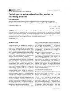
The use of a transpiration condition is useful for the application of the descent with a fixed mesh. But it may introduce inaccuracies in the numerical description of the shape being computed. In particular, transpiration approximation is known as producing an inaccurate flow when the amplitude of the shape perturbation to account for in terms of surface displacement and orientation is not small. Now, the progression towards optimal shape is generally combined with an non-negligible increasing of the amplitude. In [14], it is proposed to recover flow accuracy by updating the mesh at the end of every optimization step. The new mesh is fitted to the shape. This is obtained by a mesh deformation system relying on a spring analogy introduced in [9]. This combines two advantages, first the flow at the beginning of each optimization iteration is evaluated without transpiration, and, second, this also holds for the optimum context when shape update is converging to zero. In that case, in the set of three optimality conditions, state and adjoint are not affected by the transpiration simplification. Only the stationarity of functional (“gradient is zero” in case of non-constraint) is influenced by the transpiration approximation. This strategy is summarized in Algorithm 3: Algorithm 3: dynamic adaptation/gradient step with mesh deformation: Input: M0 , γ0 Output: M, γopt , the converged mesh and optimal shape 1- Do 2- Do 2.1- compute on current mesh the flow (state equation), 2.2- compute on current mesh the adjoint state, 2.3- compute on current mesh the (exact)gradient of functional, 2.4- perform descent: update shape control variable 2.5- compute the intersection of metrics for each intermediate flow in steps 2.1-2.3, 2.6- build a new mesh specified by the intersected metric and by a fixed number N of nodes, While adaptation is not converged. Compute a deformed mesh conforming the new shape While control is not optimized. Finally, the optimization/adaptation platform can be represented as in figure 1.

4

Applications to problem under study

Preliminary optimization computations have been applied to an HISAC test case (figure ??). We describe in Table 1, the initial configuration used to perform the pseudo-strong and the strong coupling computations. Both strategies use mesh deformation introduced in Algorithm 3. Further details can be found in [20].

Mesh

Flow Solution

W

Adjoint Solution

Fonctionnal and derivatives

( ∂ Ψ/ ∂W )*

Gradient Repeat the Design Cycle until Convergence

Steepest descent Metrics intersection Re−meshing Solution interpolation

Repeat mesh adaptation until Convergence

Shape and mesh modification

Figure 1: Strong coupling platform Initial mesh vertices size Initial mesh elements size MACH number Angle of attack Aircraft length Observation plane Number of optimization iterations Number of mesh adaptation iterations by one optimization iteration

42120 223657 1.6 3 30m z = −R = −30m 10 5

Table 1: simulation parameters Applications are based on optimizing for minimum initial shock pressure rise (ISPR) using transpiration conditions and torsional springs deformation. Minimizing the ISPR leads not only to the lowest ISPR but also to the lowest maximum overpressure.

4.1

Application of pseudo-strongly coupled scheme to coarse meshes:

A pseudo-strongly coupled scheme consists in using slightly the mesh adaptation process in the optimization platform, which means that we apply just a single time the mesh adaptation process by iteration of optimization. The aim of this exercise is to measure the impact of mesh adaptation in shape optimization platforms. Figures below, represent some comparisons between the original and the optimized configurations.

Figure ?? shows the horizontal cuts of pressure value at z = −30m in order to compare the initial flow and the final flow after optimization. We observe that the first shock localization of initial flow is slightly reduced. Figure 2 shows on the right the evaluation of functional during the coupled loop. The oscillations observed in the functional curve are associated to the re-meshing stage. On the other hand one notes that with the last iteration, a brutal descent of the function. This behavior lets us to raise questions about the certainty of the functional computation. On the left of the figure 2 we depict the progress obtained on the near-field pressure after optimization. The red line (green line) corresponds to the initial (final) near-field pressure respectively. Figure 3 shows the reduction obtained after propagation of the near-field pressure to the ground. Figure ?? shows the final pressure distribution and adapted mesh respectively. Figure 4 shows from the left to the right a comparison between the original and the optimized shapes at the nose tip respectively.

pressure analysis at z=-30 0.286

pressure before pressure after

0.285 0.284

4.2e-05

0.283

4.1e-05

0.282

4e-05

0.281

3.9e-05

0.28

3.8e-05

0.279

3.7e-05

0.278

3.6e-05

0.277

3.5e-05

0.276

cost evaluation

4.3e-05

Cost

pressure

Cost evaluations 4.4e-05

25

30

35 40 45 50 55 x-axis probe under the aircraft at z=-30

Pressure comparison

60

65

3.4e-05

0

1

2

3

4 5 6 Number of evaluations

7

8

9

Cost evaluation test-case 3: lf ront = 25 and lback = 35.

Figure 2: Pseudo-strong coupling. Left: Comparison of the near-field signatures for the original and the optimized configurations, right: cost function evaluation around coupled mesh adaptation and optimization loop.

4.2

Application of strongly coupled scheme to coarse meshes:

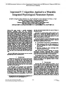
A strongly coupled scheme consists in using a sufficiently converged fixed-point mesh adaptation process in the optimization loop. Figure ?? shows the horizontal cuts of pressure value at z = −30m in order to compare the initial flow and the final flow after optimization. We observe that the first shock localization of initial flow is well reduced. Figure 5 shows on the right the evaluation of functional during the coupled loop. The oscillations observed in the functional curve are associated to the mesh adaptation phase which is devoted to find the best adapted mesh and then ensure the good evaluation of the functional. This mesh adaptation influence over global optimization loop gives us a computation certainty along optimization cycle. On the left of the figure 5 we depict the progress obtained on the near-field pressure after optimization. The red line (green line) corresponds to the initial (final) near-field pressure respectively. Figure 6 shows the reduction obtained after propagation of the near-field pressure to the ground. Figure ?? shows the final pressure distribution and adapted mesh respectively. Figure 7 shows from the left to the right a comparison between the original and the optimized shapes at the nose tip respectively. We summarize the ground signatures obtained with the pseudo-strong coupling and the strong coupling strategies in the following table:

Analysis of the sonic boom signature 70

pressure before pressure after

60

pressure in Pascal

50 40 30 20 10 0 -10 -20 -30 0

20

40

60 time in ms

80

100

120

Test case 3: H = 45000f t Figure 3: Pseudo-strong coupling: comparison of the ground signatures for the original and the optimized configurations.

baseline shape

optimized mesh

Figure 4: Pseudo-strong coupling: comparison of the original and optimized shapes at the nose tip for the HISAC case case Original shape Optimized shape by pseudo-strong coupling Optimized shape by strong coupling

ISP R(P a) 42 37.5 35

Table 2: Initial shock pressure rise in Pascal for different strategies. These results suggest that coupling strategies are suited for minimizing the ISPR. The sonic boom is reduced in both cases by creating a blunt nose (figs. 4 and 7). In particular the strong coupling strategy is more efficient than the pseudo-strong coupling strategy. Indeed, the gain reached by SC (strong coupling) is about 20% and the gain reached by PSC (pseudo-strong coupling) does not exceed the 12%.

pressure analysis at z=-30 0.286

Cost evaluations 5.2e-05

pressure before pressure after

0.285 0.284

4.8e-05

0.283

4.6e-05

0.281

Cost

pressure

0.282

0.28

4.4e-05 4.2e-05

0.279

4e-05

0.278

3.8e-05

0.277

3.6e-05

0.276 0.275

cost evaluation

5e-05

25

30

35 40 45 50 55 x-axis probe under the aircraft at z=-30

60

65

Pressure comparison

3.4e-05

0

10

20 30 40 Number of evaluations

50

60

Cost evaluation test-case 3: lf ront = 25 and lback = 35.

Figure 5: Strong coupling: Left: Comparison of the near-field signatures for the original and the optimized configurations, right: cost function evaluation around coupled mesh adaptation and optimization loop. Analysis of the sonic boom signature 70

pressure before pressure after

60

pressure in Pascal

50 40 30 20 10 0 -10 -20 -30

0

20

40

60 time in ms

80

100

120

Test case 3: H = 45000f t Figure 6: Strong coupling: Left: comparison of the ground signatures for the original and the optimized configurations, right: comparison of the near-field signatures for the original and the optimized configurations

baseline shape

optimized mesh

Figure 7: Strong coupling: Comparison of the original and optimized shapes at the nose tip for the HISAC case

4.3

Application of strong coupling with finer meshes

We recompute the above optimum with a finer specification of the number of nodes. This number is now fixed to 100,000 nodes. Cost function evaluation 5.2e-05

cost function

5e-05 4.8e-05

cost value

4.6e-05 4.4e-05 4.2e-05 4e-05 3.8e-05 3.6e-05 3.4e-05 3.2e-05

0

10

20

30

40

50

60

70

80

90

100

Number of iterations

Strong coupling, fine mesh: Optimization of the HISAC shape with a mesh size of 100Kcells

Strong coupling, fine mesh: Optimized shape: adapted mesh

Optimized shape

5

Concluding remarks

We have addressed a design problem in which mesh adaptation is mandatory. It can be considered as an equality constraint, in complement of the state system. Observing that this constraint is strongly nonlinear, we studies fixed point strategies in order to couple more or less strongly the adaptation process and the optimisation loop. This has been applied to a sonic boom mitigation study. Some of our numerical experiments show that when choosing strong coupling, the optimization can be successfully performed. In the presented application, mesh adapted optimisation brings information of higher quality than before. We are expecting an extra improvement by introducing a goal-oriented adaptation criterion.

6

Acknowledgements

We acknowledge for the support of this work by FP6-HISAC European project.

References [1] Alauzet F., Loseille A., Dervieux A. and Frey P., “Multi-dimensional continuous metric for mesh adaptation”, 15th Int. Meshing Roundtable’, Birmingham, USA, Springer Verlag, pp. 191-214, 2006. [2] Alauzet F., George P.L., Mohammadi B., Frey P., Borouchaki H., “Transient fixed point based unstructured mesh adaptation”, Int. J. Numer. Methods in Fluids, 43:6-7, 729-745, 2003. [3] Choi, S., Alonso, J. J., and Van der Weide, E., “Numerical and Mesh Resolution Requirements for Accurate Sonic Boom Prediction of Complete Aircraft Configurations”, AIAA Paper 2004-1060, 2004. [4] Nadarajah S.K., Jameson A., Alonso J., “Adjoint-Based Sonic Boom Reduction for Wing-Body Configurations in Supersonic Flow”, The Canadian Aeronautic and Space Journal, 51:4, 187-199, 2005. [5] Becker R., “Adaptive Finite Elements for Optimal Control problems”, Habilitation thesis, Universit¨at Heidelberg (2001)

[6] Beux F., Dervieux A. (Eds), “Shape Design in Aerodynamics, Parameterization and sensitivity”, European Journal of Computational Mechanics, 17:1-2 (2008) `de P.-H., Koobus B., Dervieux A., “Positivity statements for a Mixed-Element-Volume scheme on [7] Courne fixed and moving grids”, European Journal of Computational Mechanics, 15:7-8, 767-799, 2006. [8] Farhat C., Maute K., Argrow B. and Nikbay M., “A shape optimization for reducing the sonic boom initial pressure rise”, AIAA Journal, 10:10, 2091-2093, 2007. [9] Degand C. and Farhat C., “A three-dimensional torsional spring analogy method for unstructured dynamic meshes”, Comput. Struct., 80 (2002) 305. ¨t L., Va `zquez M., Dervieux A., “Automatic Differentiation for Optimum Design, applied to Sonic [10] Hascoe Boom reduction”, Proceedings of the International Conference on Computational Science and its Applications, ICCSA’03, Montreal, Canada, V.Kumar et al., editors, LNCS 2668, pp 85–94, Springer, 2003 [11] Loseille A., Dervieux A., Frey P. and Alauzet F., “Achievement of global second order mesh convergence for discontinuous flows with adapted unstructured meshes”, 18th AIAA Computational Fluid Dynamics Conference, Miami (FL), 25 - 28, 2007 [12] Nadarajah S. K. and Jameson A., “Optimum shape design for unsteady three- dimensional viscous flows using a non-linear domain method”, 24th Applied Aerodynamics Conference, June 2006, San Francisco, California. `zquez M., Koobus B. and Dervieux A., “Multilevel Optimization of a supersonic aircraft”, Finite [13] Va Element in Analysis and Design, 40, 2101-2124, 2004. `zquez M., Dervieux A. and Koobus B., “A methodology for the shape optimization of flexible wings”, [14] Va Engineering Computations, 23:4, 344-367, 2006. [15] Marco N., Koobus B. and Dervieux A. “An additive multilevel preconditioning method and its application to unstructured meshes”, INRIA research report 2310, 1994 and Journal of Scientific Computing, 12, no 3, 233-251, 1997 [16] Alauzet F., Borel-Sandou S, Daumas L., Dervieux A., Dinh Q., Kleinfeld S., Loseille A., Mesri ´ G., “Multi-model and multi-scale optimization strategies”, European Journal of Computational Y. and Roge Mechanics, 17:1-2 247-273 (2008) [17] Maute K., Farhat C., Argrow B. and Nikbay M., “Sonic boom mitigation vis shape optimization using an adjoint method and application to a supersonic fighter aircraft”, European Journal of Computational Mechanics, 17:1-2 217-243 (2008) [18] Courty F. and Dervieux A. “Multilevel functional Preconditioning for shape optimisation”, I.J.Comput. Fluid Dynamics, 20:7,481-490,2006 [19] Martinelli M., “Sensitivity Evaluation in Aerodynamic Optimal Design”, Ph.D thesis, Scuola Normale di Pisa and universit´e de Nice-Sophia-Antipolis, 2007. [20] Mesri Y. “Gestion et Contrˆ ole des maillages non structur´es Anisotropes, Applications en A´erodynamique”, Ph.D thesis, Universit´e de Nice-Sophia-Antipolis, 2007 (in french).