to hold the entry 1100X. With this information, the cost can be calculated and ... ship between all basic blocks, profiling information at the basic block level, and.
A Flexible Code Compression Scheme using Partitioned Look-Up Tables Martin Thuresson, Magnus Själander, and Per Stenstrom
Department of Computer Science and Engineering Chalmers University of Technology S-412 96 Göteborg, SWEDEN
Wide instruction formats make it possible to control microarchitecture resources more precisely by the compiler by either enabling more parallelism (VLIW) or by saving power. Unfortunately, wide instructions impose a high pressure on the memory system due to an increased instruction-fetch bandwidth and a larger code working set/footprint. This paper presents a code compression scheme that allows the compiler to select what subset of a wide instruction set to use in each program phase at the granularity of basic blocks based on a pro�ling methodology. The decompression engine comprises a set of tables that convert a narrow instruction into a wide instruction in a dynamic fashion. The paper also presents a method for how to con�gure and dimension the decompression engine and how to generate a compressed program with embedded instructions that dynamically manage the tables in the decompression engine. We �nd that the 77 control bits in the original FlexCore instruction format can be reduced to 32 bits o�ering a compression of 58% and a modest performance overhead of less than 1% for management of the decompression tables. Abstract.
1
Introduction
Traditional RISC-like Instruction-Set-Architectures (ISAs) o�er a fairly compact coding of instructions that preserves precious instruction-fetch bandwidth and also makes good use of memory resources. However, densely coded instructions tend to increase the e�ciency gap between general-purpose processors (GPPs) and tailor-made electronic devices (ASICs) by not being capable of �nely controlling microarchitecture resources. In fact, with the advances in compiler technology it is interesting to let wider instructions expose a �ner-grain control to the compiler. Very-Long-Instruction-Word (VLIW) ISAs do exactly this by exploiting parallelism across functional units, whereas architectures with exposed control such as NISC [1] and FlexCore [2] do it in order to expose the entire control to the compiler, thereby having a potential to reduce the e�ciency gap between GPPs and ASICs. In fact, recent VLIW ISAs such as IA-64 [3] use 128-bit instruction
2 bundles containing three instructions each and FlexCore uses as many as 109 bits per instruction. The downside of wider instructions, however, manifests itself in at least three ways: a higher instruction-fetch bandwidth, a larger instruction working-set, and a larger static code size. This may lead to higher power/energy consumption as well as lower performance, which may in fact outweigh the gains of more e�cient use of microarchitecture resources. Previous approaches to maintain the full expressiveness of wide instruction formats and yet reducing the pressure on the memory system have been to code frequently-used wide instructions more densely. Mips16 [4] and ARM Thumb [5] provide a more dense alternative instruction set and it is possible to switch between the wide and dense instruction formats. In another approach, a dictionary is provided that expands a densely coded instruction into a wide instruction either by coding a single wide instruction with a denser codeword [6, 7] or by coding a sequence of recurring wide instructions with a denser codeword [8�11]. Regardless of the approach, the drawback of all these schemes is that they can only utilize a fraction of the expressiveness of the wide instruction format either because only a subset is compressed or because of the huge dictionaries needed, which can incur signi�cant run-time costs. Our aim is a more scalable approach that can accommodate large programs. This paper contributes with a novel code-compression scheme that utilizes the full expressiveness of the wide instructions by coding the program in a dense fashion. The decompression engine comprises a set of look-up tables (LUTs), each used to compress a partition of the wide instruction word. The compression is done o�-line at compile-time by analyzing what subset of the wide instruction set is used in each basic block through a pro�ling pass. We present an algorithm for compression of the program using dense instructions and for management of the decompression engine at run-time by changing the dictionary entries on-the�y and yet keeping the run-time costs low. The end result is a decompression methodology that can utilize the full expressiveness of the wide instruction format with low run-time costs. The paper also presents a methodology for how to con�gure and dimension the decompression engine under various constraints such as keeping the latency of LUTs at a low level. Based on the FlexCore [2] architecture, we show that the original 77-bit instruction word can be reduced by 58% with less than 1% percent run-time cost in the number of executed instructions for manipulating the LUTs for a set of media benchmarks from the EEMBC suite [12]. As for the rest of the paper, Section 2 describes our baseline architecture model, the FlexCore architecture, followed by a description of the new compression scheme in Section 3. In Section 4, a method for selection of the con�guration of the LUTs is presented, and in Section 5 an algorithm for generating the compressed program is shown. The experimental methodology and results are presented in Sections 6 and 7, respectively. Related works are discussed in Section 8 and the paper is concluded in Section 9.
3 2
FlexCore
FlexCore [2] is an architecture with exposed control, based on the functional units found in a typical �ve-stage general-purpose pipeline. The data-path consists of a register �le, an arithmetic-logic unit (ALU), a multiplier, a load/store unit and a program-control unit connected to each other using a fully connected interconnect and controlled using a wide control word. Figure 1 shows an illustration of the architecture, with the control on top, and the interconnect at the bottom of the �gure. One unique property of the FlexCore architecture is that it is possible to include hardware accelerators in the framework and use the interconnect and the general control to �exibly con�gure a pipeline out of the available datapath elements. Another novel aspect of FlexCore is that its control space is a superset of a traditional �ve-stage general-purpose processor (GPP), making it possible to fall back on traditionally scheduled instructions found in load/store architectures such as MIPS R2000, if needed.
Control Imm
PCop
LS Unit
ALU
ImmSel
Ready
LS Size
ALUop
OpA OpB WrAddr WrEn
PC Unit
MULT
LSB
OpA OpB
MSB
DATA Reg
Address Data
DATA Reg
RegB
OpA OpB
DATA Reg
RegA
DATA Reg
DATA Reg
Interconnect Addresses
Register File
Interconnect
Fig. 1. FlexCore, an architecture using a wide control word, a fully connected interconnect, and the datapath units found in a typical early �ve-stage load/store architecture such as MIPS 2000.
While this architecture has been shown to be more e�cient in terms of execution time and cycle count for embedded benchmarks than a �ve-stage singleissue pipelined GPP counterpart, the cost in instruction-fetch bandwidth is three times higher compared to a traditional GPP like MIPS R2000, and almost as much in terms of static code size [2]. This makes FlexCore a suitable target architecture for code compression schemes, especially since embedded devices usually have very tight constraints on memory usage and power/energy consumption. The full control word for the FlexSoC, which consists of 109 signals (out of which 32 comprise the immediate values), can be seen in Table 1. So 77 of the 109 bits are for control, which is the target in this study.
4 Signal name Description
Size Signal name Description
Size
RegReadA
Reg. A read address
5
PCOp
PC operation
3
RegAStall
Reg. A read stall
1
PCStall
PC stall
1
RegReadB
Reg. B read address
5
I_ALUA
Inter. ALU A
4
RegBStall
Reg. B read stall
1
I_ALUB
Inter. ALU B
4
RegWrite
Reg. write address
5
I_RegWrite Inter. Reg write
4
RegWE
Reg. write-enable
1
I_LSWrite
4
Inter. L/S Write
Buf1
Buf1 write-enable
1
I_LS
Inter. L/S address
4
Buf2
Buf2 write-enable
1
I_Buf1
Inter. buf 1
4
ALUOp
ALU operation
4
I_Buf2
Inter. buf 2
4
ALUStall
ALU stall
1
I_CtrlFB
Inter. ctrl feedback
4
Mult stall
LSOp
L/S operation
2
MultStall
LSSize
L/S size
2
MultEnable Mult enable
1 1
LSStall
L/S stall
1
I_MultA
Inter. mult A
4
PC
PC immediate select
1
I_MultB
Inter. mult B
4
Table 1. Control signals in the FlexCore architecture. Size given in number of bits.
3
The Instruction Compression Scheme: Overview
The compression scheme leverages on the fact that during phases of the execution, some combinations of control bits will never appear in the instruction stream. Since the expressiveness found in the wide instructions is thus not utilized, a more e�cient encoding scheme can be used. The encoding scheme uses look-up tables (LUTs) to store bit patterns and the compressed instruction is a list of indexes into these tables. The bits found in the tables are then merged to form the decompressed instruction, which can then be executed. Figure 2 shows a decompression structure with four LUTs that together generate the wide instruction. Because of the simple logic involved, and relatively small LUTs needed, we will later show that decompression can be done with virtually no performance overhead as part of the instruction fetch. The contents of the LUTs can be changed using dedicated table-manipulating
instructions in the instruction stream. This allows the compiler to use small tables, whose contents are tuned for the particular phase of the execution. The placement of these dedicated instructions will a�ect the quality of the �nal solution. The static number of table-manipulating instructions will a�ect the static code size, whereas the number of table-manipulating instructions in the dynamic instruction stream will a�ect the performance overhead in terms of instruction overhead and potentially more instruction-cache misses. In this study, we adopt a straight-forward strategy � a single table-manipulating instruction, called a LUT-load, updates a single entry in one look-up table. While this makes our results pessimistic in terms of the overhead caused by the table-manipulating instructions, we note that this is an area for improvement that is subject for future research.
5
Fig. 2.
The instruction-decompression structure encompassing a number of
LUTs that expand di�erent parts of the narrow instruction into the wide complete control word.
An important design trade-o� in this scheme is the size and con�guration of the LUTs. The instruction size depends on both the number of tables, and the size of each. The number of tables dictates the number of indices in the narrow instruction format, and the number of entries dictates the number of bits needed for each index. Also, the size of the tables will in�uence how often the contents of the tables need to be updated. In the next section, we present a methodology for dimensioning the decompression engine taking this into account. The methodology also takes into account that many bits in the control word are so called �don't-care� values meaning that they can be set to either zero or one, without a�ecting the correctness of the program. Don't-care signals have previously been used successfully in the NISC project [6]. The FlexCore-compiler has been updated to generate programs where the �bits� can be 0, 1 or X, giving the compression algorithm additional opportunities for optimizations.
4
A Method for Wide-Instruction Partitioning
In this section, we present a methodology to dimension the compression-engine tables with respect to the number of tables, the number of entries in each table, and the partitioning of the wide instructions across the tables. Since the tables are �xed in the architecture, this design decision needs to be done before fabrication, and is thus done only once. The method consists of four steps, each one illustrated with examples using the FlexCore control word. In the �rst step, the designer identi�es bits in the control word that are highly correlated and should always be placed in the same LUT. These sets of bits are called sub-groups. Table 2 lists the sub-groups identi�ed in the FlexCore architecture. In the next step, all possible subsets of the set of sub-groups are generated to create possible LUT candidates. A candidate is a set of bits that together could become a LUT in the design. An optimization is to already here remove candidates which will not be in the �nal solution; for example if they are too narrow or too wide. In FlexCore, for example, we might decide to only consider
6 Sub-group Signals included
Size Sub-group Signals included
Size
RegA
RegReadA + RegAStall
6
Buf
Buf1 + Buf2
2
RegB
RegReadB + RegBStall
6
I_ALUA
I_ALUA
4
RegW
RegWrite + RegWE
6
I_ALUB
I_ALUB
4
PC
PC + PCOp + PCStall
5
I_RegW
I_RegWrite
4
ALU
ALUOp + AluStall
5
I_LS
I_LSWrite + I_LS
8
LS
LSOp + LSSize + LSStall
5
I_Buf1
I_Buf1
4
I_Buf2
I_Buf2
Mult
MultStall + MultEnable I_MultA + I_MultB
10
I_CtrlFB I_CtrlFB
4 4
Table 2. Sub-groups for the FlexCore architecture. Size given in number of bits.
candidates with a width between 7 and 16 bits because of delay and power constraints. Here (RegA, RegB) is a candidate, but (Buf, I_Buf ) is too narrow to be a reasonable one, since too many small LUTs lead to a lower degree of compression. In the third step, LUT candidates are combined into groups called possible
solutions, so that the candidates in the group cover all the bits in the control word once, and only once. One of many possible solutions in our example is the following candidate list: (I_RegW, I_LS, RegW), (I_ALUB, I_Buf2), (I_ALUA, Mult), (LS, PC), (ALU, I_CtrlFB Buf, I_Buf1) (RegB, RegA). Finally, each of the possible solutions is evaluated using a user-de�ned cost function. The cost function evaluates how good the possible solution is for a given application (called workload), and returns a numerical result (lower is better). This makes it possible to �nd a solution that is relevant for the type of applications that will be executed on the system. In our experiments, we have used cost functions for LUT-access time, compressed instruction width, and energy e�ciency. Several cost functions can be given with di�erent priority, and only if a high priority function ties, a lower is evaluated. This makes it easy to add hard design-constraints, such as a maximum access time for the tables, and to make sure that the design �ts within a given power envelope. The cost function will take the LUT con�guration into account given by the possible solution, and calculate the LUT sizes needed for the workload, so the whole program can be executed without inserting LUT-loads. In the LUT size calculation, don't-care bits are greedily set to 0 or 1 if it makes it possible to merge two entries into the same value. For example, if the LUT already holds the entry 1X00X, and we try to add the entry X100X, the LUT would be updated to hold the entry 1100X. With this information, the cost can be calculated and returned. Once all the possible solutions have been evaluated, the designer is presented with a list of the solutions with the lowest cost. While each run of the algorithm gives a list of solutions tuned for that particular workload, we propose running it several times with di�erent workloads. Among all the saved solutions, the designer can pick one that works well for all of the workloads.
7 One challenge in this methodology is to �nd a suitable workload. The workload should, for the best solutions, produce LUTs that have a size that results in an acceptable access time and power consumption. For the benchmarks used in this paper, we selected a subset of the full program by running the EEMBC benchmarks one iteration (using the �ag -i1 ) and all the program counter-values for the executed instructions were recorded. For each benchmark, the footprint used was the subset of instructions selected by the program-counter trace. The algorithm also reports the size needed for each suggested LUT. Since the compressed program can change the contents of each LUT, the distribution of the sizes can be used to determine the �nal sizes for the LUTs.
5
Algorithm for Generation of a Compressed Program
In order to execute a program on a system using our proposed compression scheme, the generated binaries need to be updated by inserting the LUT-load instructions inside the binaries. We have developed an algorithm for generating a compressed program with the LUT-loads placed to keep the performance penalty low. One important approach is to avoid placing LUT-loads in basic blocks that are frequently executed, such as inside inner loops. Since the original wide instructions are compressed, it is possible to reduce the instruction footprint size. A pro�ling run is used to get the execution frequency for the basic blocks. We can then estimate the performance overhead caused by the LUT-loads simply by multiplying the number of required table manipulations in each basic block with that block's execution count. In order to generate the �nal compressed program, the algorithm uses the uncompressed program, a compiler-generated �ow graph showing the relationship between all basic blocks, pro�ling information at the basic block level, and the LUT-table con�guration. The algorithm uses the �ow graph as its main data structure and it associates a complete list of entries with each basic block that are needed in the tables for the basic block to be executed. An entry in this context means a value that is present in a LUT in this basic block. If any basic block requires more entries than the capacity of the tables, the basic block is split into several basic blocks. The algorithm uses three �ags, while updating the �ow-graph. The �ag L (Load), is used for any entry that does not exist in all of the possible predecessors to a given basic block. It is signi�cant since only entries that are marked with L will actually generate LUT-load instructions. The �ag N (Needed) shows that an instruction in the basic block requires the entry to be present in the LUT. These entries can never be removed from the basic block, since the code would not work without it. Finally, the �ag X (Locked) is used by the algorithm to tag an entry as processed. This makes it easy to process the entries one-by-one, and make sure that all are visited once, and only once. Initially, all entries in the �ow-graph are scanned, and the L and N �ags are set according to the description above. Figure 3(a) shows a �ow-graph for
8 Name: BB1 Exec: 1
Name: BB1 Exec: 1 001010 (LX)
Name: BB2 Exec: 5 001010 (LN)
Name: BB3 Exec: 1 001010 (N)
(a) Before optimization
Fig. 3.
Name: BB2 Exec: 5 001010 (NX)
Name: BB3 Exec: 1 001010 (NX)
(b) After mization
opti-
Example of a simple �ow-graph used to illustrate the algorithm. The
graphs show the locations a particular entry in one of the LUTs before and after BB2 is optimized.
a simple loop used to illustrate the algorithm, with each basic block annotated with its execution count from the pro�ling run. Also, the entry 001010 for one particular LUT is shown with its �ags. The entry is initially stored in two di�erent basic blocks, but only marked with L in BB2, since the only path into BB3 is through BB2. The performance penalty for this particular state is �ve, since a LUT-load in BB2 would be executed �ve times. The next step of the algorithm will process the entries marked with L oneby-one, until all have been processed. The main idea behind the algorithm is to look at one entry at a time to see if it is possible, with a lower cost, to make sure the entry already exists in of the possible predecessors. This is done using a recursive optimization function that works as follows. For each entry that is marked L in the graph, the optimization function tries to �push� the entry to all the predecessors of the basic block. The pseudo-code in Figure 4 shows on a high-level how the function works. It keeps track of the cost as it pushes the entry to the predecessors and returns the best cost it can. The algorithm continues to recursively push the entry further until one of several conditions occur: 1) the value already exists in a basic block; here don't-care values are greedily resolved to zeros or ones, if it helps to �nd a match 2) the table in the basic block is full; 3) it reaches a root node in the graph; or 4) a maximum recursion depth has been reached. If the minimum cost found is smaller than the current cost, the new entries are added to the a�ected basic blocks and all the �ags are updated. Being able to push entries marked with L out of loops is essential for getting a well performing solution. Since each optimization may increase the number of entries in the LUTs, the entries in the basic blocks that have the most L-�ags are processed �rst. To keep the execution time of the algorithm down, the recursive depth should be set. This bounds the computational complexity, which would otherwise be
9 // Calculate possible cost achieveble by (recursively) moving // entry up to all predecessors optimizeLoad(current_node, entry) if(recursionLevel > MAX || current_node.IsRootNode() == 0) return INT_MAX cost = 0; loop over predecessors using pred if(pred.HasEntry(entry) cost += 0 elseif(pred.IsFull()) return INT_MAX // No room to push the entry else cost_here = pred.ExecutionCount() // Cost if not pushed further cost_push = optimizeLoad(pred, entry) // Cost if pushed further if(cost_here