mains besides railways including airlines, hotels, call centers, hospitals, and sports ..... node in the graph has both incoming and outgoing arcs; some nodes also ...
Annals of Operations Research 127, 259–281, 2004 2004 Kluwer Academic Publishers. Manufactured in The Netherlands.
A Flexible, Fast, and Optimal Modeling Approach Applied to Crew Rostering at London Underground MANMOHAN S. SODHI
Cass Business School, City University London, UK STEPHEN NORRIS
London Underground, UK
Abstract. We present a general modeling approach to crew rostering and its application to computerassisted generation of rotation-based rosters (or rotas) at the London Underground. Our goals were flexibility, speed, and optimality, and our approach is unique in that it achieves all three. Flexibility was important because requirements at the Underground are evolving and because specialized approaches in the literature did not meet our flexibility-implied need to use standard solvers. We decompose crew rostering into stages that can each be solved with a standard commercial MILP solver. Using a 167 MHz Sun UltraSparc 1 and CPLEX 4.0 MILP solver, we obtained high-quality rosters in runtimes ranging from a few seconds to a few minutes within 2% of optimality. Input data were takes from different depots with crew sizes ranging from 30–150 drivers, i.e., with number of duties ranging from about 200–1000. Using an argument based on decomposition and aggregation, we prove the optimality of our approach for the overall crew rostering problem. Keywords: crew rostering, rota, mixed-integer linear programming, cyclic graph, decomposition, aggregation
1.
Introduction
We present a fast and flexible approach to crew rostering at London Underground. Aiming at flexibility, speed, and optimality, the approach is unique in that it succeeds in achieving all of these. This general approach decomposes the overall problem into stages, two of which are solved with a general mixed integer linear programming (MILP) solver, and the others are handled with graph-theoretic or even manual approaches. Large mass transit systems like London Underground are complicated not only because of the multitude of management considerations, labor laws, and union requirements, but also because requirements have been changing rapidly in the recent past. Moreover, with repairs being made continually on an ageing infrastructure, timetables need to be altered at short notice, thus requiring daily duties (hence, duty sheets) and crew rosters to be altered quickly as well. Thus, although crew rostering at the Underground has been done manually with great skill for over a century, crew depot consolidation and changing requirements made it necessary for the management to consider flexible computer-assisted approaches.
260
SODHI AND NORRIS
Due to evolving rules at the Underground, flexibility was the main goal for us while speed and optimality are always desirable in a planning system. To achieve these goals, we decompose the problem of creating a roster – this is called a rota at the Underground owing to the rotation of drivers on the roster – into stages that can be solved easily using a standard MILP solver, not a specialized algorithm. Future changes in requirements are expected to entail changes only in the models but not in the solvers, thus providing a flexible approach. The two main stages in our approach reflect the existing manual process: (1) create rest-day pattern including shifts, and (2) assign duties to the rest-day pattern thus obtained. The focus of this article is the first stage that we further decompose into three steps: (1a) Across all depots, set up a single graph with allowed weekly and multi-week patterns of rest days and shifts as nodes and allowed week-to-week transitions as arcs. (1b) Use a MILP model whose input include this graph and user-preferences and solve it to yield the specific patterns that comprise an “optimal” rest-day pattern for a particular depot. (1c) Construct a rest-day pattern using a simple graph-theoretic heuristic using the output of the previous step for the depot under consideration. We did (1a) manually as this is needed just once across all depots, but it could also be done using heuristics or constraint programming in systems other than the Underground. For step (1b) we used a commercial MILP solver, CPLEX 4.0, on a 167 MHz SunSparc Ultra 1 machine and solved it within 2% of optimality in runtimes ranging from a few seconds to a few minutes depending on the size of the depot (30–150 drivers). For the final step (1c), we used a depth-first search algorithm that took a fraction of a second to find the first rest-day pattern; we did not investigate developing all the rest-day patterns. We model the second stage as an assignment problem with side-constraints, and we solve it in a matter of seconds even for large crew depots with 100–150 drivers using the same solver. Deployment of a decision support system based on this approach is pending the development and deployment of computer-assisted enhancements to train timetabling and to duty sheet generation that would provide the duties for input to crew rostering. This article contributes in three ways. First and foremost, in a problem space in which algorithms and models tend to be highly specialized because every crew-rostering system is unique, it describes an approach that is simple, flexible, and hence has potential for adaptation to systems other than the Underground. Second, it offers the possibility of theoretical advancement. It is unusual in this domain to even aim at optimality leave alone achieve it so we therefore hope our optimal approach will encourage others to seek optimal solutions for practical problems. Third, it adds to the OR literature on crewrostering by describing an application at a large complex system like the Underground. 2.
Literature survey
Ernst et al. (2001) survey staff scheduling including crew rostering in a variety of domains besides railways including airlines, hotels, call centers, hospitals, and sports. Ow-
FLEXIBLE, FAST AND OPTIMAL MODELING APPROACH
261
ing to the complexity of staff scheduling, they observe that researchers usually decompose these problems by solving them in stages. Our approach also has stages in this regard, but different from the ones suggested by them. Among different approaches for mass transit systems, for instance, EmdenWeinert, Kotas, and Speer (2001) describe a crew rostering system for tram and bus drivers at the Bremer Straßenbahn AG in Germany. Their proposed system for rostering is different than that at the Underground. They propose dividing up the drivers and duties at a depot into groups, and developing rotas for each group separately. Recently some Underground depots are reportedly interested in experimenting with multiple rotas as well, so their work on assigning duties to different groups of drivers within the same depot and assigning drivers to different groups may potentially be applicable to these Underground depots. The “rota” in their case is, in our terms, only the pattern of rest days and shift types. They use MILP for assigning shifts to cells of the rota, an approach we rejected early on because solution time grows exponentially with problem size. Indeed, even for a tiny rota for 12 drivers, they report truncating the run after 28 hours without finding an optimal solution, and find one for a 6 drivers only after six hours using CPLEX 6.5. Contrast this to seconds and minutes of runtime on much larger problems (30–150 drivers) we obtained with on a likely slower machine and an older version of the same solver, CPLEX 4.0. However, Caprara et al. (1998) obtained good runtimes by using a heuristic informed by the relaxation of a MILP model. Their target problem, presented in a competition by the Italian railway company, Ferrovie dello Stato SpA, is slightly different: given a number of duties, determine a roster that minimizes the number of weeks with each duty being done everyday. Like us, they define a graph, but the nodes are duties in contrast with patterns in our case; the use of patterns allows us to incorporate complicated constraints that cannot be expressed in their graph. Compared to their model, our MILP models are simpler and do not need relaxation or specialized heuristic for solving. A different train-related crew rostering situation is reported by Ernst et al. (2000), who present the modeling approach they took with the Australian railway, National Rail. Drivers have to contend with long driving distances so that each run is a shift in itself and drivers may stay at barracks. The situation is similar to airline crew management but has important differences. All possible roundtrips for National Rail can be enumerated and used as input, so many hard constraints around round trip construction can be embedded into the roundtrip generation program. This can be compared with stage (1a) of our approach where all weekly or multi-week patterns are enumerated taking into account hard constraints applying to these patterns. They have a system-wide model for crew scheduling that outputs roundtrips and the number of drivers at each depot. Subsequently, they model crew rostering at the depot level and use a MILP model. However, to solve this model in reasonable time, they are forced to relax the integrality constraints and to round up the resulting continuous solution to obtain an integer solution; this is questionable practice but possibly appropriate in their practical context. Constraint programming is a technique that has been deployed recently and software vendor ILOG’s web site (www.ilog.com) has a few articles from their users’
262
SODHI AND NORRIS
conference on crew rostering applications, e.g., nurse rostering, that were developed using their software. We tried ILOG’s software but our experience indicated that constraint programming is not useful when there are linear constraints involving many variables as in the present situation. Possibly because of this reason, hybrid approaches using constraint programming and MILP have been suggested recently for general-purpose problems; see, for instance, Jain and Grossman (2001). Ernst et al. (2001) discuss this briefly in their survey and provide a couple of references reporting hybrid application for crew rostering. Our approach may be considered a hybrid approach as well in the sense that steps (1a) and (1c) are amenable to constraint programming while step (1b) is a MILP model. We did not use constraint programming ourselves because generating all the patterns and transitions in (1a) is a one-off problem easily handled manually. Generating a rota from the MILP output in (1c) is easily handled with a simple graph-theoretic heuristic. But systems other than the Underground may benefit from applying constraint programming to these steps. Based on their survey, Ernst et al. (2001) reflect that existing crew-rostering models and algorithms are highly specialized and therefore there is a need for general approaches. Our method may be one way to meet this need because we believe it can be adapted for rotation-based crew-rostering in systems other than the Underground. 3.
Crew rostering at London Underground
As part of its operations planning, London Underground does timetabling, crew scheduling, and crew rostering. Timetabling produces plans for specific runs of trains on the different lines each starting at a certain point on the line at a certain time and arriving at different stations on specified times. Crew scheduling results in detailed daily duties, assuming generic drivers from different depots, to man all the train runs produced by timetabling. Each duty, a sequence of train runs to man with breaks, is one day’s work for one driver. Finally, crew rostering assigns specific drivers at each depot a sequence of duties for the next so many weeks. 3.1. Rota We are specifically concerned with crew-rostering here and the output of this step is a table – see table 1 for an example – called a rota. The person responsible for creating a rota for a crew depot is called a rota compiler. The columns of this table represent the consecutive days of a week, Sunday through Saturday. The rows represent consecutive weeks and there are as many rows as there are drivers for the depot in question. Every cell in a rota has one of the following: a specific duty identified by its number, a generic rest duty that represents a day off, or a generic leave cover duty to cover for drivers who are on leave that day. Although a specific duty encompasses many tasks and breaks, for the purpose of rostering, the only relevant information is (1) the duty number to identify the particular duty, (2) the start or book-on time, (3) the end or book-off time, and (4) the
FLEXIBLE, FAST AND OPTIMAL MODELING APPROACH
263
Table 1 Example of a crew roster (rota) for a hypothetical 10-driver depot. ‘R’ in some of the cells signifies a rest day while the other cells have (1) duty number, (2) start time, (3) end time, and (4) duration for the duty to be performed. Note the four-day weekend going from week 004 to week 005. Week
Sun
Mon
Tue
001
** Leave cover A ** – hours 72:00
002
** Leave cover B **
Wed
Thu
Fri
Sat
Total hrs 72:00
003
R
068 15:04 23:14 07:40
068 15:04 23:14 07:40
067 15:01 22:21 06:50
R
067 15:01 22:21 06:50
060 16:30 11:58 06:58
35:58
004
044 16:07 21:27 04:50
108 14:55 23:18 07:43
108 14:55 23:18 07:43
108 14:55 23:18 07:43
108 14:55 23:18 07:43
R
R
35:42
005
R
R
014 05:59 13:39 07:10
014 05:59 13:39 07:10
014 05:59 13:39 07:10
014 05:59 13:39 07:10
017 06:53 14:49 07:26
36:06
006
R
102 10:52 18:28 07:06
102 10:52 18:28 07:06
102 10:52 18:28 07:06
102 10:52 18:28 07:06
R
034 10:15 18:13 07:28
35:52
007
052 21:47 06:32 08:15
090 22:38 06:13 07:05
090 22:38 06:13 07:05
090 22:38 06:13 07:05
090 22:38 06:13 07:05
090 22:38 06:13 07:05
R
43:40
008
030 14:01 22:03 07:32
059 14:13 21:40 06:57
059 14:13 21:40 06:57
059 14:13 21:40 06:57
R
R
R
28:23
009
R
R
033 07:04 15:29 07:55
033 07:04 15:29 07:55
041 10:52 16:26 05:04
102 10:52 18:18 06:56
078 09:29 18:06 08:07
35:57
010
023 09:02 16:20 06:48
042 11:02 18:18 06:46
R
R
033 07:04 15:09 07:35
033 07:04 15:09 07:35
026 07:53 16:05 07:42
36:26
duration from start to end. (See any cell in table 1 that has a specific duty.) Each duty is specific in the sense that starting times and durations can differ from duty to duty. Contrast this to simpler systems like hospitals or retail stores where all early duties may have the same starting times and the same ending times. This specificity of duties adds to the complexity of crew rostering in the case of the Underground. Simple standard shifts,
264
SODHI AND NORRIS
e.g., 8 am–5 pm and 12 pm–10 pm, could simplify crew rostering at the Underground, but would increase costs by increasing idle time. At any depot, each driver is assigned a different row on the rota so he knows the duty identification number for each day of the week that is not a rest day. The number of rows is the same as the number of drivers so each gets a separate row. The driver also knows the duties for future weeks because in the subsequent week, he gets the next row down the rota, and in the following week, the row below that. After he finishes the last row of duties for some week, he rotates up to the first row of the rota; this rotation explains the word ‘rota.’ The same is true for all other drivers except that they are working different rows in any given week. Rotation reflects fairness in the following sense: if there is a particularly undesirable or desirable sequence of weeks in the rota, all drivers will eventually get their turn to work those weeks. This contrasts with seniority or other preference-based systems for assigning week-on-week duties. Consider the example in table 1 for a hypothetical depot with 10 drivers. Most depots have many more drivers, some exceeding 150. Suppose a driver has week 4 this week. He would do duty 044 on Sunday, duty 108 on each day Monday through Thursday, followed by rest days on Friday and Saturday. In the following week, he would do week 5 on the rota. He will start with two rest days, thus getting a four-day weekend Friday through Tuesday. Thus, even though each week (row) has exactly two rest days, with exceptions related to weeks with night duties, it is possible for a driver to get long weekends of three, four, or even five days as rest days at the end of one week are juxtaposed with rest days at the beginning of the following week. In fact, the tradeoff between more regular or two-day weekends versus fewer but more desirable long weekends with three or four consecutive days off is something with which the depot manager and hence the rota compiler has to contend. 3.2. Shifts and rest-day pattern Let us understand shifts at the Underground first. Based on its start and end times, a duty has a shift: early (E), late (L), and night (N). The duty is an early shift if it begins between 12:01 am and 11:59 am; a late shift if it begins some time between 12:00 pm and 8:59 pm; and a night shift if it begins between 9:00 pm and 12:00 midnight. The day-off or rest duty is denoted by ‘R.’ A central concept is that of the rest-day pattern that comprises the placement of rest days and the types of shifts or duty-types for the rota. Many of the Underground’s requirements apply specifically to the pattern of duty-types within a week. For instance, it is not desirable to have any week containing mixed duty types so it may comprise only E’s and R’s, an early week. The subsequent week may be required to have only L’s and R’s and is called a late week. A mixed week comprises both early and late duties and is to be avoided as a soft constraint. Table 2 exemplifies the rest-day pattern for the example in table 1: weeks 3 and 4 are late weeks followed by two early weeks, 5 and 6. Week 7 is a night week but is considered a late week when making a pattern of week types.
FLEXIBLE, FAST AND OPTIMAL MODELING APPROACH
265
Table 2 Rest-day pattern for rota from hypothetical example in table 1. Besides the placement of rest days (R) and leave cover duty (C), the shift type of the remaining cells is determined to which specific duties with matching shifts can be assigned later. Week
Sun
Mon
Tue
Wed
Thu
Fri
Sat
Week type
001 002 003 004 005 006 007 008 009 010
C C R L R R N L R E
C C L L R E N L R E
C C L L E E N L E R
C C L L E E N L E R
C C R L E E N R E E
C C L R E R N R E E
C C L R E E R R E E
– – Late Late Early Early Late Late Early Early
3.3. Existing manual approach to crew rostering The rota compiler manually creates a crew roster or rota in two stages: 1. Create rest-day pattern. The rota compiler assigns only a rest day or the type of duty to each cell in the rota: early, late, or night, resulting in a rest-day pattern exemplified by table 2. His goal is to maximize the weighted sum of the number of regular weekends, two consecutive days off not including weekends, and long weekends, the weights reflecting the preferences of the depot manager. The procedure is as follows. The rota compiler places night weeks and cover weeks and marks each week as being ‘early’ or ‘late’ depending on the past pattern at this depot or as desired by the depot manager. He then places rest days and early or late duties by trial-and-error ensuring that the total number of duty types is not violated; some compilers do this for Saturday and Sunday columns first and then fill out the rest of the rest-day pattern. The last step is to try swaps between weeks to increase the number of weekends. The number of rest days is precomputed as a proportion of workdays and guarantees a feasible solution. 2. Assign specific duties. Given a rest-day pattern, the rota compiler (manually) assigns a specific duty number to each cell of early, late, or night type, matching the type of duty to cell duty type assigned earlier. E.g., if duty number 068 starts at 15:04, it can only be put in a cell that has a late duty type assigned to it in the rest-day pattern. Feasibility is ensured by the number of different duty-types in the rest-day pattern matching that of the duty-types of the specific duties. The rota compiler’s effort goes into swapping different assignments across weeks to improve the quality of the assignments by decreasing the violations of such soft constraints as the work for each week being close to 36 hours. The first stage is crucial for crew satisfaction as this is where the placement of rest days, and hence the number of regular and long weekends, is determined. The rest-day
266
SODHI AND NORRIS
pattern is more than just intermediate output: the rota compiler discusses it with the depot supervisor as part of the process to get the rota approved. 4.
Objectives and constraints
The primary objective creating a rota for a depot at the Underground is to maximize the weighted sum of regular weekends, of pairs of consecutive days off not including weekends, and of long weekends; the weights reflect the preferences of the depot manager. The secondary objective is to minimize the violation of soft constraints for the specific duty assignment. We present the overall problem in two subsections corresponding to creating a rest-day pattern and to assigning duties. 4.1. Rest-day pattern Objective function (R1) Maximize the weighted sum of the number of two non-weekend consecutive days off, of the regular weekends, of three-day weekends, and of four-day weekends. Constraints on creating a rest-day pattern (R2) Two rest days will be rostered every week except for a week of night duties when no rest day will be rostered until nights are completed; normally four rest days in week following nights. (R3) Leave cover weeks, computed on the basis of one for every six crew members, rounded up, should be paired except when there is an odd number of leave cover weeks. (From March 2003 onwards, the basis is two for every thirteen crew members.) Furthermore, cover duties should be spread over the rota. (R4) There should be no more than seven days of consecutive duty (soft constraint), and under all circumstances no more than ten days of consecutive duty (hard constraint). (R5) Preferably work same shift all week. Mixed weeks are sometimes possible with a maximum of one transition from an early to a late duty hence this is a soft constraint. (R6) Maintain the shift pattern for the depot. The shift pattern is the pattern of the types of weeks – early and late primarily – in the rota. It should not be confused with the rest-day pattern or with the “pattern” of duties within a week. The shift pattern may be an early week followed by a late week and then an early week again, i.e., an early–late pattern. Or, it may alternate with pairs of early weeks with pairs of late weeks, an early–early–late–late shift pattern. For large depots, four early weeks may alternate with four late weeks, an E–E–E–E–L–L–L–L shift pattern. Mixed and night weeks are viewed as late weeks for the purpose of falling into a shift pattern. It may be necessary to break the pattern in some
FLEXIBLE, FAST AND OPTIMAL MODELING APPROACH
267
cases, so this requirement is a soft constraint. (As of this writing, some depots are considering multiple rotas at the same depot comprised of early weeks only, of late weeks only, of extreme late and night weeks only, as well as mixed shift patterns such as the ones discussed above. Thus each rota is made for a group of drivers at the depot rather than for the entire depot. The problem of optimally splitting a depot into such groups is not considered here; see Emden-Weinert, Kotas, and Speer (2001) instead. The present approach can be a step in creating multiple rotas.) Based on the pattern, weeks are classified as early or late weeks. (R7) Precede and follow leave cover weeks with a rest day. (R8) Avoid rest days split by one day. For instance, a shift pattern with rest duties on Monday and Wednesday in any week, or on Saturday of one week and on Monday of the following week is not allowed. (R9) Avoid consecutive Sundays booked on duty (except for weeks with cover duty). (R10) An implicit requirement is that the number of different types of duties must match the sum of appropriate duty type assignments. 4.2. Assigning duties Objective The objective here is to minimize the violation of soft constraints. Constraints for assigning duties (D1) Each driver will work 36 hours per week within user-specified tolerance error ε of, say, 30 minutes. A night week and a week immediately following a night week is an exception to this rule. This is a soft constraint. Furthermore, all working weeks should be as close to each other as possible. So, if the duties are such that average workweek is less (or more) than 36 hours, then we use that number instead. (D2) The total number of hours for every rolling 8 week period will be within ±5% of 8 × 36 = 288 hours. (The number 288 can be replaced by 8 × average workweek if different from 36 hours.) (D3) A minimum of 12 hours will be rostered between finishing work on one day and starting work on the following day. This applies only to non-leave cover weeks. (D4) A pair of leave cover weeks is rostered to work as the longest pair of (non-leave cover) rostered two weeks. (However, for the purpose of creating the rota, we took the desired weekly average instead.) (D5) Booking-on times for duties in a week should be similar. Moreover, in an unbroken sequence, early duties should start progressively later as the week progresses, while late duties should end progressively earlier. In practice, the user specifies a parameter τ (say, 15 minutes) to require a difference of at least that much between book-on (or book-off) times of consecutive duties as a soft constraint.
268
5.
SODHI AND NORRIS
Proposed solution method and model
Creating a monolithic model encompassing all the constraints is undesirable because solving such a model would be quite a challenge and because at least part of it, the second stage of assigning duties, is an assignment problem with side constraints that is solved quickly with a standard MILP solver. Given that the first stage is quite hard to solve on its own, there is no point in making it harder by adding the complexity of the second part in a monolithic model. Therefore, our proposed computer-assisted approach preserves the existing manual approach by decomposing the problem into two corresponding stages: the first to create a rest-day pattern and the second to assign specific duties to the rest-day pattern obtained from the previous stage. In many systems other than the Underground, the second stage may be trivial or absent. For the second stage, we modeled assigning specific duties for a particular rest-day pattern as an assignment problem with side constraints. This MILP model assigns specific duties to the duty types in each cell using binary variables to denote an assignment of specific early duties to early cells, specific late duties to late cells, etc. by weekday. It is straightforward to incorporate constraints (D1)–(D5) as side constraints to this assignment problem when hard and as an objective when soft. Interestingly, this second step, though easily modeled and quickly solved with a computer, is quite tedious and difficult for manual solution especially in light of some of the newer constraints like early book-ons (D5) to be progressively late as the week progresses. Despite having about 22,000–33,000 binary integer variables for depots with crew sizes ranging from 100 to 150, respectively, the model solves in a few seconds for optimality within 98%. Due to the straightforward nature of this model, we will not discuss it further in the present article. Instead, we focus on the stage 1 problem of creating a rest-day pattern. 5.1. Overall approach for stage 1 Note three things about the stage 1 objectives and constraints. (1) There are two types among (R1)–(R10): those involving the specific pattern of rest days and shifts within a week and those involving the transition from one week to another. For instance, the (soft) constraint of same duty types applies to a week, while that of rest days preceding and following leave cover weeks involves transitions from another week into the leave cover week and from a leave cover week into any other week. (2) For a driver, a rota is a rotation or cycle comprising weekly (or multi-week) pattern of duties. He does one week, goes on to the next, and so on, finally arriving back at the starting point. (3) The same weekly pattern may occur repeatedly in different weeks for a given rest day pattern. Motivated by this, we can view a rest-day pattern as a cyclic subgraph on a directed graph whose nodes are allowed weekly (or multi-week) patterns and whose arcs are allowed transitions; these are the same for all depots. The hard (i.e., inflexible) constraints can then be embedded in the graph and the soft constraints and objectives can be taken into account when attempting to find a cyclic path that maximizes the user’s preferences, that minimizes the penalties on soft constraints, and that meets the rota-specific
FLEXIBLE, FAST AND OPTIMAL MODELING APPROACH
269
constraints. Thus we decompose the overall problem of creating a rest-day pattern into three steps: (1a) Set up a directed graph of patterns and transitions manually (one time setup); (1b) Identify patterns and transitions in this graph for the required rest-day pattern using a MILP model; and (1c) Construct a rest-day pattern in its familiar form using depth-first (or other) search on the subgraph identified in previous step. 5.2. Step (1a): Create a directed graph This step involves a one-time specification across all depots of feasible weekly (or multiweek) patterns of duty-types and the allowed transitions between these. This specification incorporates the hard constraints from the set (R2)–(R10) as applicable. The resulting graph is common to all rotas from any depot and serves as input for generating a specific rest-day pattern. For the Underground, the allowed weekly (multi-week) patterns were identified manually and the allowed transitions were computer-generated using AMPL. Consider a graph G(N, A) each of whose nodes in set N is a weekly or multi-week pattern complying with within-week (or extended to multiple weeks with multi-week patterns) constraints from (R2)–(R10). Figure 1 shows the graph conceptually. Table 3 gives some examples of allowed and disallowed patterns: only allowed nodes comprise the set N. Next consider the arcs, i.e., the transitions from one weekly or multi-week pattern to another. The directed arc from pattern p to pattern q, both from N, is in A if the transition is feasible in accordance with hard constraints from the set (R2)–(R10). Every node in the graph has both incoming and outgoing arcs; some nodes also have self-arcs
Figure 1. The graph with patterns (nodes) and transitions (arcs) that are allowed in accordance with hard constraints for rest-day pattern creation. Each node is a single or a multi-week pattern, e.g., EEEEERR or LLRRLLL–RREEEEE.
270
SODHI AND NORRIS
Table 3 Examples of allowed and disallowed weekly as well as multi-week patterns. Hard constraints for within-week patterns are embedded into the allowed patterns. Soft constraints and objectives are ignored. Pattern EERREEE REREEEE LEELERR REEREEE NNNNNR EERREEE EERRRRE ELLLLRR
Allowed? Yes No; rest days split by 1 No; mixed duties Yes Yes; night duties Yes (two week pattern) Yes; one switch from E to L is acceptable
Table 4 Examples of allowed and disallowed weekly and multi-week patterns. Hard constraints for transitions from one pattern to another are embedded into the allowed transitions (arcs). Soft constraints and objectives are not taken into consideration. From-pattern
To-pattern
Transition allowed?
EERREEE RREEEEE EEEEERR REEREEE NNNNNNR
RREEEEE EEEEERR RRLLLLL RLLLRLL RRRLLLL
EERREEE EERRRRE ELLLLRR EEERREE
EERREEE EERRRRE EEEEERR EEERREE
Yes No, ten consecutive workdays Yes; has a four-day weekend as well Yes Yes; week of night duties to be followed by week with three rest days Yes, but will not be preferred at a depot that desires an early–early–late–late pattern Yes Yes; thus, some self-arcs are allowed
that are considered as both incoming and outgoing. Table 4 gives examples of allowed and disallowed arcs. 5.3. Step (1b): Identify patterns and transitions for rest-day pattern Having embedded all the hard constraints common to all depots in the previous step of constructing the graph, we now have to deal with the depot-specific soft constraints and objectives in order to construct an “optimal” rest-day pattern. There are two reasons for considering the use of MILP for this step. One is that MILP is good at finding a provable global optimum compared to heuristics like simulated annealing, simulation, genetic algorithms, etc. The other reason is that after incorporating the hard (inflexible) constraints into the graph in the previous step, we are left with linear soft constraints and a linear objective function.
FLEXIBLE, FAST AND OPTIMAL MODELING APPROACH
271
Thus, we seek a MILP model (M1) for step (1b). A cyclic path corresponding to a rest-day pattern must be such that the total number of visits to all nodes (accounting for those corresponding to multi-week patterns) should equal the number of weeks in the rota. Likewise, the number of incoming arcs for the “optimal” rest-day pattern must equal the number of outgoing arcs. Self-arcs – an arc from a node to itself – count as both incoming and outgoing arcs. Finally, if we assign weights to different patterns and transitions in accordance with the desirability (or undesirability) of their inclusion in the “optimal” subgraph (hence, rest-day pattern), the objective function (and violation of soft constraints) becomes linear in the number of arcs and nodes. Recall the graph G(N, A) from the previous step. Then, the problem of identifying which particular patterns (nodes) and transitions (arcs) comprise an “optimal” subgraph given the particular rest-day pattern requirements. From this subgraph, we will extract a rest-day pattern in step (1c). Indices and sets i: the index to the set of all patterns (nodes) N = {1, 2, . . . , i, . . . , |N|}. j: the index to the set of all transitions (arcs) A = {1, 2, 3, . . . , j, . . . , |A|}. d: the index to the set of days of the week {Sunday, Monday, . . . , Saturday}. Ain (i): the subset of A with arcs that are inbound to node i. Aout (i): the subset of A with arcs that are outbound from node i. (A self-arc at node i is both inbound and outbound.) Parameters Ii,R,d : number of rest days in pattern i, day d. Ii,E,d : number of early days in pattern i, for day d. Ii,L,d : number of late days in pattern i, for day d. Ii,N,d : number of night duties in pattern i, for day d. Wi : number of weeks in the pattern i (multi-week patterns entail 2 or more weeks). Inputs R: the number of weeks in the rota, same as the number of drivers. KR,d : total number of rest duties for day d of the rota. KE,d : total number of early duties for day d of the rota. KL,d : total number of late duties for day d of the rota. KN,d : total number of night duties for day d of the rota. KC : total number of leave cover duty weeks for the rota. Pi : user-provided preference weight for node i based on whether or not the node entails two nodes off or whether it entails a mixed week. Qj : user-provided preference weights (or negative of penalty) of arc j based on the type of weekend involved on whether the arc fits the shift pattern. Decision variables mi : number of times node (pattern) i is present in the “optimal” rota. nj : number of times arc (transition) j is present.
272
SODHI AND NORRIS
Then the resulting MILP model is: MILP model (M1). Max
�
Pi mi +
�
i
s.t.
�
Qj nj = z1 ,
(1)
j
Wi mi = R,
i
mi −
�
(2)
nj = 0,
∀i ∈ N,
(3)
nj = 0
∀i ∈ N,
(4)
Ii,R,d mi = KR,d
∀d,
(5)
Ii,E,d mi = KE,d
∀d,
(6)
Ii,L,d mi = KL,d
∀d,
(7)
Ii,N,d mi = KN,d
∀d,
(8)
j ∈Ain (i)
mi − �
�
j ∈Aout (i)
i
� i
� i
� i
�
Wi mi = KC ,
(9)
i∈NC
R � mi � 0, integer
∀i ∈ N,
(10)
R � nj � 0, integer
∀j ∈ A.
(11)
In this model, (1) is the objective function to identify those nodes and arcs whose (multiple) inclusion would maximize preference. In practice, the weights are computed based on the type of node or arc, for instance, the user may specify the weight for threeday weekends, in which case all arcs corresponding to a three-day weekend are assigned the same weight. Constraint (2) ensures that the total weeks spanned by the selected nodes equals the size of the rota. Constraints (3) and (4) ensure the cyclic nature of the rota by requiring the number of visits to incoming and outgoing arcs respectively into node i are equal to the number of times the node is visited. These constraints form the majority of constraints and are also highly sparse. Constraints (5)–(8) require that, for each day of the week, the total number of duties for various types equal the selected patterns provide for that day. For instance, if the rota has 25 rest duties on Sunday as determined at the end of crew scheduling, then the selected patterns must be such that together they contribute 25 rest duties for Sunday. These are 4 × 7 constraints in all. Constraint (9) ensures that the selected patterns in node subset NC , i.e., with cover duty, be such that together they equate the total number of leave cover weeks needed.
FLEXIBLE, FAST AND OPTIMAL MODELING APPROACH
273
Figure 2. Conceptual example showing the nodes and arcs that comprise the optimal subgraph as determined by the MILP model. The numbers next to the nodes indicate how many times that node should appear in any “optimal” rest-day pattern to which this subgraph maps.
Finally, the integrality constraints (10) and (11) require the numbers of patterns visits to be non-negative and integer, i.e., 0, 1, 2, 3, etc. bound from above by the number of weeks, R. Although we used this upper bound, a tighter upper bound for each pattern i is the maximum number of times this pattern can possibly appear based on the number of different duty-types for each day, i.e., as the minimum of K∗ ,d /Ii,∗ ,d over ∗ = R, E, L, N and over all days d. The output of this model identifies an optimal subgraph and the number of times each node (and arc) in this subgraph is visited by the cyclic graph that maps to one or more “optimal” rest-day patterns. See figure 2 for a conceptual example; broken lines indicate that the corresponding node or arc is not part of the optimal subgraph. Computational experience Our experimental tests conducted in 1996–1997 on a 167 MHz SunSparc Ultra 1 with data from small and large crew sizes (30–150) show that this approach generates rest day patterns in times ranging from several seconds to a few minutes for 98% optimality. The size of the MILP model is the same regardless of any particular rota because it is determined by the graph that is common to all rotas. The number of variables, all general integer, is equal to |N| + |A|, i.e., the number of nodes and arcs, and the number of constraints is essentially 2|N|. For one-week and two-week patterns, there are about |N| = 500 nodes and |A| = 100,000 arcs, all represented by integer variables. The relatively small number of constraints (∼1000) ensures the problem is solved fast. However, the solution time increases with the increase in right-hand side corresponding to crew size. We used CPLEX 4.0 as the MILP solver and AMPL for modeling. Coding was done in C++ with executables developed using Sun’s own C++ compiler.
274
SODHI AND NORRIS
Figure 3. A conceptual rota developed from the output of the MILP model in step 2. The rest-day pattern has patterns d–f–h–a–d–f–g–b–a, and after the last pattern, the rotation goes back to pattern a as indicated by the broken arrow, which is also included as a transition.
5.4. Step (1c): Create rest-day pattern This is the final step to construct a rest-day pattern from the output of the MILP model in step (1b) that identifies the patterns and transitions in the rest-day pattern along with how many times each is to be included. From this output, many rest-day patterns can be constructed given that many of the weekly patterns (and transitions) are present more than once in the MILP solution. All of these have the same objective value (stage 1) as described in step (1b). A depth-first search algorithm can used to generate some or all the possible rest-day patterns. In our implementation, we generated only the first one. There may be reasons, not included in the model, for a rota compiler to select one rest-day pattern over another; one such reason is the relative placement of leave cover weeks. This step takes only a fraction of a second for generating the first rest-day pattern, so generating more or even all, should not be time-consuming. But rather than the rota compiler poring over all these variations, we would recommend an interactive approach of obtaining a desirable rest-day pattern by letting the rota compiler pick a starting node and then subsequent nodes upon being shown what choices he has next. We did not implement an interactive method ourselves. Figure 3 shows a conceptual rota developed in this step taking the output of the MILP model in the previous step.
6.
Optimality
Optimality is a way to ensure solutions that are consistently of high quality. With staged decomposition, we need to prove optimality. We start with Assumption 1. The duties provided are such that a feasible rota exists.
FLEXIBLE, FAST AND OPTIMAL MODELING APPROACH
275
It follows therefore that a feasible rest-day pattern and feasible duty assignment to this pattern exists but we can make a stronger statement. Lemma 1. For any feasible rest-day pattern, there exists a feasible duty assignment resulting in a feasible rota. Proof. Duty assignment to a rest-day pattern (stage 2) comprises of assignment constraints as hard constraints and a number of soft constraints. Because the duty types for creating a rest-day pattern (stage 1) are obtained from the duties, a number of assignments can be made from duties to their respective duty types in the given feasible rest-day pattern. These obey the hard constraints. � This means that once we have a feasible rest-day pattern, we know that a feasible duty assignment exists. This and the following lemma make decomposition possible. Lemma 2. An optimal rota’s rest-day pattern is also optimal. Proof. The objective function for a rota comprises two parts corresponding to the entailed rest-day pattern and the duty assignment, respectively. The former can be weighted arbitrarily more. So if an optimal rota’s rest-day pattern were not optimal, an improved rest day pattern could be used to obtain an improved rota. But that would mean that the given rota is not optimal. � Theorem 1. Decomposition using first a procedure to create an optimal rest-day pattern and then a procedure to assign duties optimally results in an optimal rota. Proof. From assumption 1, we know that a feasible rest-day pattern exists so a procedure to create an optimal rest-day pattern would indeed find one. From lemma 1, we know that we can obtain an optimal assignment of duties as well. It follows then from lemma 2 that the resulting rota is optimal because if this were not the case, we would be able to find an improved rest-day pattern from a better rota than the one obtained. � So we are left with having to prove that the stage 1 and state 2 procedures satisfy the conditions of theorem 1. We have the following two theorems that do that. Theorem 3. Stage 2 assigns duties optimally to any feasible rest-day pattern. Proof. This is trivial as the stage 2 problem is a MILP that solves optimally if the problem is feasible. Feasibility follows from lemma 1. � Theorem 4. Stage 1 results in an optimal rest-day pattern. Proof.
See next subsection.
�
276
SODHI AND NORRIS
Assuming the truth of theorem 4 – we shall prove it shortly – we can use theorems 1, 3, and 4 to obtain Theorem 5. Stages 1 and 2 applied consecutively produce an optimal rota. We are thus left with proving only theorem 4 that we prove next using an aggregation-based argument. 6.1. Stage 1 optimality We prove the optimality of stage 1 in three steps. First, we provide a MILP model (M2) that would provide an optimal rest-day pattern if solved. Second, we show that step (1a) aggregates this MILP model to (M1) that we actually solve in step (1b), and that step (1c) disaggregates the resulting solution to fit the original MILP model. Third, we show that the optimal solution from the aggregated model, when disaggregated, is also optimal for the disaggregated model. Thus, steps (1a), (1b), and (1c) produce an optimal solution. The aggregation here is a row-and-column aggregation. There are no known results pertaining to the optimality of the disaggregated solution of an aggregated general MILP model when both columns and rows are aggregated. Our result is possible only because of the special structure of (M2). To obtain (M2), revise steps (1a), (1b), and (1c) to steps (1a ) and (1b ) in the following manner. In (1a ), construct a graph G (N , A ) in which each pattern appears as a node R times or at least as many times as the tighter bound mentioned earlier. Let the subset of nodes corresponding to pattern i be Ni . Corresponding to each arc in G, create all-to-all arcs in G between the nodes corresponding to the two patterns when different. For any arc j = (i, k) with i �= k in G, let A j be the subset of G with arcs Ni × Nk . For arc (i, i) in G, create arcs from a node to all the other nodes corresponding to the same pattern but not to itself in G . For each transition j = (i, i) in G, let A j be the subset of arcs in G such that A j = Ni × Ni − {(i, i) | i ∈ N }. In step (1b ), define (M2) similar to (M1) in step (1b) with the important difference that each node or arc can appear at most once in the solution. Index and sets Ni and A j : described above. N and A: the set of patterns and transitions, respectively, as before. i and j : index over N and A, respectively, as before. k: index over any set of replicated patterns Ni . l: index over any set of arcs A j . Decision variables xik : binary variable indicating inclusion for node corresponding to pattern i replication k. yj l : binary variable indicating inclusion for the l th element of arc set A j for transition j .
FLEXIBLE, FAST AND OPTIMAL MODELING APPROACH
MILP model (M2). Max
�
Pi
�
i
s.t.
�
xik +
k
�
Wi
i
�
Qj
277
�
j
yj l = z2 ,
(1 )
l
(2 )
xik = R,
k
xik −
�
yj = 0
∀i ∈ N, ∀k ∈ Ni ,
(3 )
yj = 0
∀i ∈ N, ∀k ∈ Ni ,
(4 )
xik = KR,d
∀d,
(5 )
xik = KE,d
∀d,
(6 )
xik = KL,d
∀d,
(7 )
xik = KN,d
∀d,
(8 )
j ∈A in (i)
�
xik − �
j ∈A out (i)
Ii,R,d
i
�
k
Ii,E,d
i
�
Ii,L,d
i∈NC
� k
Ii,N,d
i
�
� k
i
�
�
� k
Wi
�
(9 )
xik = KC ,
k
1 � xik � 0, integer 1 � yj l � 0, integer
∀i ∈ N, ∀k ∈ Ni , ∀j ∈ A, ∀l ∈ A j .
(10 ) (11 )
The solution to this MILP is a cyclic path with each included node (or arc) appearing exactly. We have then by construction. Lemma 4.1. An optimal solution for the model (M2) is an optimal rest-day pattern relative to the stage 1 objective function. � We can obtain (M1) by aggregating constraints and variables in (M2). Aggregate the constraints (3 ), (4 ), and (10 ) over k in Ni as well as constraint (11 ) over l in A j . Then, aggregate the variables by making the substitutions: � xik = ni ∀i ∈ N, (S1) k∈Ni
�
yj l = mj
∀j ∈ A.
(S2)
k∈A j
The result is (M1) obtained as a row-and-column aggregation of model (M2). Through this aggregation, we are aggregating graph G (N , A ) to G(N, A) as well. The next two lemmas compare the solutions of the two models.
278
SODHI AND NORRIS
Lemma 4.2. For any feasible solution in (M2), there exists a feasible solution in the aggregated model obtained using summations (S1) and (S2) with the same objective function value. Proof. Suppose (x, y) is a feasible solution of (M2). Making the substitutions (S1) and (S2) to get (m, n), it follows from inspection that (m, n) satisfies the constraints � of (M1). We also have z1 (m, n) = z2 (x, y). Lemma 4.3. For any feasible solution in (M1), there exists a feasible solution in the original model (M2) with the same objective function value. Proof. Any feasible solution to the aggregated model (M1) can be disaggregated using the following disaggregation procedure D: 1. Let (m, n) be a feasible solution to the aggregated model (M1) with associated graph G(N, A). Construct graph G(N , A ) and model (M2) with variables x and y. 2. Set x = 0, y = 0. 3. For all patterns i ∈ N with mi = t > 0, disaggregate mi by setting xik = 1 for the lowest t indices, i.e., k = 1, . . . , t. (All other xik remain zero for all i and k.) 4. For all arcs j = (p, q) in A with pattern p �= q, and nj = s > 0, we must have mp � s and mq � s as well owing to constraints (3) and (4) in (M1). From the previous step, we have xpk = 1 for k = 1, . . . , mp as well as xqk = 1 for k = 1, . . . , mq . Set the variables yj l = 1 where these variables correspond to the oneto-one arcs (lexicographically) between the following two sets both of cardinality s: (1) the subset of the first s replications for which xpk = 1 and no outbound arc has a corresponding yj l set to 1 yet, and (2) the subset of the first s replications for which xqk = 1 and no inbound arc has a corresponding yj l set to 1 yet. In other words, when disaggregating the graph G to G , choose the nodes and arcs that are to be set to one based on the lowest index. Nothing precludes choosing any other lexicographic selection so this disaggregation procedure is neither special nor unique. Indeed the different paths step (1c) can generate correspond to these different procedures. � Now we can compare optimality using (M2) with that using (M1). Lemma 4.4. An optimal solution of (M1) when disaggregated using procedure D is optimal for (M2). Proof. Let (m∗ , n∗ ) be an optimal solution of (M1) and (x, y) be the disaggregated solution for (M2) obtained using procedure D. Suppose that there exists an optimal solution (x ∗ , y ∗ ) for (M2) with a better objective function value z2 (x ∗ , y ∗ ) > z2 (x, y) =
FLEXIBLE, FAST AND OPTIMAL MODELING APPROACH
279
z1 (m∗ , n∗ ). By lemma 4.2, there exists (m, n) with z1 (m, n) = z2 (x ∗ , y ∗ ) > z1 (m∗ , n∗ ), � implying therefore that (m∗ , n∗ ) is not optimal in (M2). Step (1b) produces an optimal solution for (M1) and step (1c) disaggregates this solution using procedure D or its alternatives. By lemma 4.4, we have an optimal solution to (M2) and, therefore, by lemma 4.1, an optimal rest-day pattern and the truth of theorem 4. 7.
Conclusion
Crew rostering is a complex application, in part because each system is unique. Moreover, large systems like the Underground are complex because of the crew size at each depot, the requirements stemming from management considerations, labor laws, and union demands in addition to ongoing maintenance and evolving requirements. We have described a general computer-assisted approach that, we believe, will serve not only the Underground, but also other complex rotation-based crew rostering situations where flexibility, speed, and solution quality are desirable for a computer-assisted approach. Our approach decomposes the overall crew rostering problem into stages so that general solution techniques can be applied at each stage. This also helps separate out the more easily solved portions from the harder ones. The chief benefit this approach is its flexibility. There is little custom code here and the MILP solver is off-the-shelf and is used without any tuning other than specifying the value of ε for ε-optimality. Should the requirements at the Underground change, we only need to change parameters of the models, or in the worst case, the nodes and the arcs of the graph in step (1a). Another benefit is speed not only relative to the manual solution requiring an hour or two to a few days but also in absolute terms as runtimes range from a few seconds to a few minutes. The solution quality is comparable to the best solutions that were created manually and honed over several years. Fast solution with good quality means that a compiler can generate many different rest-day patterns in a single afternoon and offer a choice to the depot manager in selecting a rest-day pattern. For the second stage assigning duties to a rest-day pattern, the MILP solver takes only a few seconds even for large depots, and besides saving time, benefits the rota compiler by reducing the tedium of this step. Achieving provable optimality for the overall crew rostering problem is noteworthy. The complexity of crew-rostering has resulted in researchers seeking heuristics based, for instance, on simulated annealing, genetic algorithms, or relaxation of integer constraints. We hope researchers will be encouraged to seek optimal algorithms, despite the daunting complexity, using either our approach or similarly motivated ones. Still, there are shortcomings. One shortcoming of our approach is its inability to handle constraints that cannot be captured at the node or arc level. Indeed, this may be an opportunity for constraint programming, especially in step (1c). One constraint, for instance, that is not handled at the node or arc level is that leave cover weeks should be spread evenly throughout the rota. Another “constraint” is that historically certain
280
SODHI AND NORRIS
night weeks or leave cover weeks were placed in certain weeks within the rota and, for any new rota, the depot manager and the drivers expect these weeks to be in the same weeks of the existing rota. It is not possible to express such a constraint in the above framework other than attempting to find a reasonably close answer by searching through all the different cycles that are possible in step (1c). Even then night weeks or leave cover weeks may not end up in the desired weeks of the rota. There is much follow up work from both practical and theoretical viewpoints. Further work at a practical level includes identification of approaches that allow the rota compiler to interactively guide the computer towards a desirable solution. We believe that the heuristic in step (1c) should be especially amenable to human guidance. Trying out different LP solution techniques and branch-and-bound approaches with the latest version of the commercial MILP software to achieve faster solution speed with smaller values of ε than the 2% value we tried is also worthwhile. Bixby (2002) provides empirical evidence that Version 7.1 of CPLEX is many times faster than the 4.0 version used for the work described here. Use of constraint programming in steps (1a) and (1c) is also worth pursuing both from a practical and theoretical viewpoint. It would also be interesting to see how a staged decomposition approach like ours can be applied to difficult problems other than crew rostering. Despite the ability of this approach to solve crew rostering for the Underground, we believe eventually the solution time would blow up if we keep increasing R, the size of the rota. As such, a study of the increase in solution time with increasing rota size would be interesting from two viewpoints: being able to project what depot sizes can this approach solve practicably, and being able to say something about delaying the blowing up of solution time of NP-complete problems by using staged approaches like the one presented here. Acknowledgments This work benefited from early discussions with Dr. Vernon Francis who suggested the key idea of working with weekly patterns. Chris Singellos was instrumental in specifying and testing the stage 2 model. The authors did this project in 1996–1997 as part of an initiative at the London Underground that had Sabre, the employer of one of the authors at the time, as the contractor. The authors would like to thank Professor Arthur Geoffrion (UCLA) for his comments especially on the section on optimality, as well as two anonymous referees and Professor Kipp Martin (University of Chicago) for comments on presentation. References Bixby, R. (2002). “Solving Real-World Linear Programs: A Decade and More of Progress.” Operations Research 50(1), 3–15. Caprara, A., M. Fischetti, P. Toth, and D. Vigo. (1998). “Modeling and Solving the Crew Rostering Problem.” Operations Research 46(6), 820–830.
FLEXIBLE, FAST AND OPTIMAL MODELING APPROACH
281
Emden-Weinert, T., H. Kotas, and U. Speer. (2001). “DISSY – A Driver Scheduling System for Public Transport.” Version 1.11, downloaded on July 11, 2002 from http://people.freenet.de/ Emden-Weinert/DISSY/DISSY-Whitepaper.html Ernst, A.T., H. Jiang, M. Krishnamoorthy, H. Nott, and D. Sier. (2000). “An Integrated Optimization Model for Train Crew Management.” Annals of Operations Research, to appear. Ernst, A.T., H. Jiang, M. Krishnamoorthy, and D. Sier. (2001). “Staff Scheduling and Rostering: A Review of Applications, Methods and Models.” European Journal of Operational Research, to appear. Jain, V. and I.E. Grossman. (2001). “Algorithms for Hybrid MILP/CP Models for a Class of Optimization Problems.” INFORMS Journal on Computing 13(4), 258–276.