A FLEXIBLE FLOW SHOP MODELLING AS A DISTRIBUTED PRODUCTION SYSTEM Rui M. Lima and Silvio do Carmo Silva Department of Production and Systems School of Engineering of University of Minho Campus de Azurem 4800-058 Guimariies - Portugal
[email protected] /
[email protected]
A model of Distributed Production Systems and a formal representation is presented applied to a flexible flow shop. This model is based on recent organizational paradigms like Holonic, Fractal and Bionic production systems. An approach to the problem of resource allocation to production units is developed.
1. INTRODUCTION All Production organizations are faced with an increased need for change, based on the necessity of reducing the time to market new products, timely delivering customer orders and dealing with increased technological evolution. These needs may be satisfied on the basis of a set of new manufacturing organization paradigms like Fractal (Warnecke, 1993), Holonic and Bionic Manufacturing Systems (Tharumarajah, Wells and Nemes, 1996; Mathews, 1995). These are organization conceptual meta-models based on autonomous production units composed of other similar units. Nowadays technology is available, based on global communications and distributed data bases and information systems, to allow efficient allocation of globally available resources and services for the production of specific products while demand subsists. This adds up to dynamically putting together distributed resources for designing dedicated and virtual production systems. One concept based on these lines, called OPIM - One Product Integrated Manufacturing, has been put forward in (Putnik and Silva, 1995). Our definition and model of Distributed Production System is closely related with this concept. Furthermore we argue that the underlined characteristics of Distributed Production Systems are the autonomy and distribution of production units or resources and possibility of frequent system reconfiguration, i.e., dynamic reconfiguration, in order to adapt to production changing requirements. In line with this view, in this work, we model a flexible flow shop as a distributed production system. This modelling adapts the flow shop studied in (Azevedo, 1999). The definition, modelling and formal
V. Mařík et al. (eds.), Knowledge and Technology Integration in Production and Services © Springer Science+Business Media New York 2002
72
Balancing Knowledge and Technology in Manufacturing and Services
representation of Distributed Production Systems here discussed are oriented for the dynamic design and operation of systems based on the above mentioned organizational and operation paradigms.
2. DISTRIBUTED PRODUCTION SYSTEM MODEL In our view (Lima, Silva and Martins, 1999) a Distributed Production Systems is composed of a network of autonomous processing units, with the possibility of dynamic reconfiguration of the production system. Three fundamental characteristics are emphasized: distribution, autonomy and reconfiguration. We can view a system as distributed if there is the need for modelling the distance between units, due to either or both information and physical communication between production units. The problem of distribution may be seen as a problem of system integration as described in (Vernadat, 1996). A platform of integration is needed for the information and physical object communication and a business model with a common semantic reference for mutual understanding of different systems. The integration problem is common to all systems. Traditionally this problem use to be addressed in large design cycles under a homogeneous design and organisational environment. We use the view of production systems integration as a more heterogeneous problem treated in small design cycles, under frequent system reconfigurations. Autonomy is a relative and not absolute characteristic related to production units. They have the autonomy to use the means of production they choose to manufacture the product as required. The autonomy is constrained by the overall system objectives. In this sense this concept respects the concept established in (Warnecke, 1993) in the Fractal Company, and as been referred in other works, namely in (Mathews, 1995). Ideally, dynamic system reconfiguration should happen instantaneously for optimal adaptation of the production system to some disturbance. In practice, however, this always takes some time which could be used as a measure of system agility. In our modelling approach, a production unit autonomously able to manufacture a product is called a cell. This is made up from either non-autonomous production units or other cells or both. A cell executes a particular service always delivering a product. This may be delivered to the next cell for further processing, handling or storage. In this sense, any kind of service may be provided by autonomous cells. This approach was initially described in (Lima and Silva, 1998). In our view, a distributed production system is designed for carrying out production of a product quantity required by some product order and ceases to exist after order completion. Such a system is made of several cells, each one, dedicated to the production of each product, i.e. component, of a product structure (Figure 1). It must be noted, that a component of the product structure is also named product. Our model of a distributed production systems is therefore a particular view of a product oriented manufacturing system (Silva and Alves, 2002), since it is specifically designed for achieving production requirements associated with a single production order of a specific product, including all it's components.
73
A Flexible Flow Shop Modelling as a Distributed Production System Production Resources
Level
CD CJ
0
0
0
0
1· 1
CD 0
0
0
~ ~
6
At "" •
level
Production Cells
Products
1· 1
6
0
Figure 1: Distributed Production System Levels
3. THE FLEXIBLE FLOW SHOP In the flow shop problem each job i (J~i~n) consists of a set of m operations Oij (J$9n) with processing times Pij, where each operation must be processed on machine Mj in the exact sequence 1 to m (Brucker, 1995). A flexible flow shop (FFS) is a generalisation of the flow shop with parallel processors at least in one stage of processing (Pinedo and Chao, 1999). The modelled FFS and alternative choices of production are shown in Figure 2, presenting a view based on production stages. The product oriented modelling view, dependent on product structure, used in this modelling approach is based on the products delivered at each production stage. Additionally we view, in a FFS, a product as the result of processing in un" production stages, considering that at each stage the input is the result of the previous stage plus, if necessary, one or more raw material or component. Stage 1
Stage 2
Stage 3
Stage 4
~ 222 3
2
3
GJ
Figure 2: A FFS example (adapted from Azevedo, 1999).
4. ALGEBRAIC REPRESENTATION Our modelling approach to distributed production systems embeds Holonic and fractal principles of systems design, considering systems inside systems, i.e., systems aggregation, to reach a final system configuration. The Generalised Scheduling work put forward in (Lecompte, Deschamps and Bourrieres, 2000), allows the formal representation of distributed production systems modelled as FFS. A formal model of FFS, seen as a distributed production system is developed,
74
Balancing Knowledge and Technology in Manufacturing and Services
representing aggregated systems, the relations between them, and the relation between the candidate resources and the tasks.
4.1 Aggregating/Disaggregating Level Mechanism In out model a high level cell, executing a task, can aggregate several other cells executing other tasks, in a fractal view of the system, as stated by our model. The product structure is the foundation of the aggregating mechanism, i.e., a cell delivering a product aggregates all services related to the delivering problem of components of that product, in our model also called products. The number of tasks in a level will always be superior to the number of tasks in the upper level, because a set of tasks will be represented in the upper level as one task. In one level the number of objects will be non-superior to the number in the immediately lower level. At the lowest, more detailed level, all objects / products, are represented and consequently all tasks responsible for delivering those objects. At the highest level, only the representation of the final product delivering service is considered, based on transformation of raw materials. In this modelling process raw materials are all production objects delivered by tasks that we do not want to control or model. Each level down will have the additional representation of the set of tasks responsible for delivering the products immediately lower in the product structure, and it is possible to have the same number of objects between levels if parallel tasks are aggregated. Levels associated with the FFS example will be represented in the forthcoming subsections. 4.2 Lower Level v=O The previous example is represented at the lowest level 0, which is the more detailed level, as the Petri net represented in Figure 3, where each task tj performed by one cell represents one stage of the FFS (Figure 2) and each object OJ represents one product. Other levels will exist, each one related to the encapsulation of the tasks in one more general task, until the upper task, which is the one that is responsible for delivering the final product.
Figure 3: Production System Lowest Level Petri Net Each Petri Net, as represented in (Lecompte, Deschamps and Bourrieres, 2000), can be associated with the transformation matrix C (equation (1.1», with elements Cjj representing object quantities consumed or manufactured by tj task. The upper index of matrices represents the level number. The quantity of work executed in a task consumes or generates objects on the system, in quantities proportional to C. So, the change of object quantities is given by the product of the quantity of work by the matrix of objects consumed-generated by the tasks. Tasks on the Petri Net are associated to a quantity of work vector W, representing the task effort necessary to deliver a desired quantity of the output objects of each task. A unitary quantity of
75
A Flexible Flow Shop Modelling as a Distributed Production System
work delivers qQ units indicated by the product structure of an object. The product structure is closely related to the level zero Petri Net of the system. In this example J~Q~12.
Pre:OxT~~; Post: 0 x T ~ ~.
;w'=[B.~]
I I CO =Post - Pre = !
'I
I!Equation !
(1.1)
I
4.3 Upper Level v=l=3 At the upper level of aggregation of cells one only cell executes a production task, delivering the final product. This final product is the same as 09 in Figure 3. This upper level can be represented by the Figure 4 Petri Net and respective C and W matrices.
°2 C3 =03
tl -ql -q2 -q5
°4 °5 °6
-qll ql2
o.
"
01
q.=q,,(level 0)
w =[w/] 3
-qg
Figure 4: Level v=I=3 cell and object representation. Task t) from Figure 4 aggregates all production system tasks, i.e., tasks t) to t4 from Figure 3. Objects 01 to 06 from Figure 4 are the same as objects OJ, 02, 04, 06, Og, 09 from Figure 3.
4.4 Level v=l-l =2 Task t) from Figure 5 aggregates tasks t) to t3 from Figure 3 and task t2 is the same as task t4 from Figure 3 and the same as task t) from Figure 4. Objects 0) to 06 from Figure 5 are the same as objects 0), 02, 04, 06, 07, Og, 09 from Figure 3. 0.
0,
°2
0, ~
"
'2
Os
0,
0,
CI ,",'
O.
=OJ
°4 Os
0.
" "
-q, -q, -q, -q. q. -q,o -qll
WI
=[~2:]
76
Balancing Knowledge and Technology in Manufacturing and Services
4.5 Level v=l-2=1
Task t) from Figure 6 aggregates tasks tl and t2 from Figure 3 and tasks t2 and t3, not aggregated, are the same as tasks t3 and t4 from Figure 3. Objects 01 to 08 from Figure 6 are the same as objects OJ, 02, and 04 to 09 from Figure 3. 0, -q, " " " 0, -q, -q,
0, 0,
0,
q.
cl:;::O.
0, ~"
0,
0,
0.
0,
-q, -q, q,
w' -qlQ
0,
-qll
0,
q"
"[:!]
Figure 6: Level v=l- J =2 cells and objects representation.
s. RESOURCE ALLOCATION In the case we are analysing in this work there are 4 tasks that can be executed by some resources for each task. The quantity of work Wjk is the task or work of type j (1 :S j :S n=O) executed by resource k (1 :S k :S r). If some resource does not execute some type of work, than the respective quantity of work is zero. Our problem resides on the assignment of resources to tasks and the assignment problem can be transformed (Hillier and Lieberman, 1989) to the transportation problem. This kind of problems has two fundamental restrictions: supply and demand restrictions. Demand restriction is related to the satisfaction of ordered quantities, named as covering restrictions in (Lecompte, Deschamps and Bourrieres, 2000). The total amount of work done by all resources involved on a task work must be equal to the required amount of work for that task as represented in equation (1.2). r +",+Wlk +",+wlr ="W; I , Equation (1.2) jk =Wj,j=l, ... ,n~ ... k=1 Will + ... + Wllk + ... + wllr =W" I Supply restriction is related to the available resource capacity, i.e., the total amount of work developed by each resource must not exceed his total capacity in all tasks he is involved with (see equation (1.3». The ajk parameter (Lecompte, Deschamps and Bourrieres, 2000) represents the total amount of work that may be accomplished by resource k on type of workj during a period of time. WXI a+ ' " + w.~ a< -1 II a, +... +W;x:,.' W. i L~::;l,k=l, ... ,r~ { ... ! Equation (1.3) j=l a jk w,J + + Wj,j + + w.J < 1 i I~, ... /a /a I Introducing a new parameter Cjko as the time for a resource k to execute one unit of work j, which we call, a unit processing time, and considering the available time of resource k represented by Tko the relation between ajk and Cjk is given by eq. (1.4). aik =7;,/cik Equation (1.4) Decision variables are integers restricted by equation (1.5). Wit ~ 0, W jk are integeres Equation (1.5)
LW
{WII
I
II
I
JI
jr
III
,..
llr -
i
I
77
A Flexible Flow Shop Modelling as a Distributed Production System
5.1 Resource Allocation Strategy The 5 fundamental steps on distributed resource allocation problems referred in (Tharumarajah, 2001) are: l.Decompose orders into operations; 2. Assign operations; 3. Select machine; 4. Allocate operation; 5. Coordinate allocation & build schedule. In this distributed production system model the 1sl step is reduced to the decomposition of one order into tasks associated to each product in the product structure. Problem 2 and 3 referred above is treated as a resource allocation at each level of aggregation and results from the replies that are received from candidate cells. The problem of finding the optimal resource allocation vector for one level of aggregation depends on the used strategy. If we want to minimize the total processing time of all resources in all tasks, than we have the minimization problem represented in equation (1.6), constrained by equations (1.2), (1.3) and (1.5), that can be solved by integer programming.
LL 11
min
f
r
C jk • wjk
j=1 k=1
I Equation (1.6) I
5.1.1 Example Considering an order of 100 units of object 09 and random object quantities qQ (Figure 3) represented at Table 1, with the objective of maintaining the stock of intermediate components it is possible to compute the quantity of work at each task, obtaining: W]=300; W2 =300; W3 =200; W4 =JOO. This would lead to the following raw materials requirements: 0] - 600; 02 - 900; 04 - 600; 06 - 800; 08 - 200. Table 2 represents random available capacities by resource for each task for a period of time.
Ta bl e 2 Aval'1 abl e capacIty b,y resource and reqUIredb y tas kf,or a penod 0 f hm ' e. Task W. Resource aik
1 (t})
300
1 (au) 2 (au) 3 (a} 3)
2 (t2)
300
4 (a2,4)
3 (t3)
200
6 (a3,6) 7 (a3.7) 8 (a3.8)
4 (t4)
100
5 «(12.5)
9 (a39) 10 (a4.1O) 11 (a4.Jl)
210 100 35 240 150 55 100 120 10 40 90
f
~
=1, for all k
Than c
jk =!ajk
The solution presented in Table 3 represents the allocation of resources to tasks by the quantity of work indicated. This is a solution for a particular random example, indicating the applicability of the model, at least, for the particular case.
78
Balancing Knowledge and Technology in Manufacturing and Services
6. CONCLUSION A fundamental problem to be solved in the design and operation of distributed production systems is the allocation of resources to different tasks to be performed. An algebraic model was used for representing a Flexible Flow Shop as a Distributed Production System. The model was applied for solving the resource allocation problem based on a particular strategy of allocation for a case study. The production system structure is modelled matching the structure of the product to be manufactured. through mechanisms of generation and boundary delimitation of sub-systems. Future work will address model test and validation using industrial and academic cases under several allocation strategies. associated with order requirements or production system objectives. These strategies may involve aspects such as parallel processing and system loading levels.
7. REFERENCES I. Azevedo, AL. Apoio a Decisao na Negocia~ao de Encomendas em Redes de Empresas. Disserta~ao para obten~ao do Grau de Doutor em Engenharia Electrotecnica e de Computadores (in portuguese). Faculdade de Engenharia: Universidade do Porto, 1999. 2. Brucker, P. Scheduling Algorithms: Springer-Verlag, 1995. 3. Hillier, FS and Lieberman, GJ.lntroduction to Operations Research: McGraw-Hill, 1989. 4. Lecompte, T, Deschamps, JC and Bourrieres, JP. A data model for generalized scheduling for virtual enterprise. Production Planning & Control, 2000; 11(4): 343-348. 5. Lima, RM and Silva, SC. Object Oriented Modelling of Product Oriented Manufacturing Systems, in
Intelligent Systems for Manufacturing: Multi-Agent Systems and Virtual Organization (LM Camarillha-Matos, H Afsarmanesh and V Marik). Prague, Czech Republic: Kluwer, 1998: 325334. 6. Lima, RM, Silva, SC and Martins, PM. Sistemas Distribuidos de Produ~ao, in }O Congresso LusoMo~ambicano de Engenharia (J FS Gomes, A Matos and C Afonso), Maputo, M~ambique, 1999; B 13-B20 (in portuguese). 7. Mathews, J. Organizational Foundations of Intelligent Manufacturing Systems - the Holonic View Point. Computer Integrated Manufacturing Systems, 1995; 8(4): 237-243. 8. Pinedo, M.and Chao, X. Operations Scheduling with Applications in Manufacturing alld Services: McGraw-Hili, 1999. 9. Putnik, GD and Silva, SC. One-Product-Integrated-Manufacturing. in Balanced Automation Systems:
Architectures and Design Methods (LM Camarinha-Matos and H Afsarmanesh), 1995. 10. Silva. SC and Alves. A. Design of Product Oriented Manufacturing Systems. in 5th IEEE IfFIP
International Conference on Information Technology for Balanced Automation Systems ill Manufacturing and Systems - BASYS'2002, Cancun. Mexico: Kluwer, 2002. II. Tharumarajah. A. Survey of resource allocation methods for distributed manufacturing systems. Production Planning & Control, 2001; 12(1): 58-68. 12. Tharumarajah, A, Wells. AJ and Nemes, L. Comparison of the Bionic. Fractal and Holonic Manufacturing System Concepts. International Journal of Computer Integrated Manufacturing. 1996; 9(3): 217-226. 13. Vernadat, F. Enterprise Modeling and Integration: principles and applications: Chapman & Hall, 1996. 14. Warnecke, HJ. The Fractal Company: Springer-Verlag. 1993.