A fluctuating hydrodynamic approach to correlation functions in two

REVISTA MEXICANA DE F´ISICA 48 SUPLEMENTO 1, 243 - 253

SEPTIEMBRE 2002

A fluctuating hydrodynamic approach to correlation functions in two phase bubble columns A. Soria,∗ E. Salinas-Rodr´ıguez,∗ J.M. Zamora,∗ Departamento I.P.H., Universidad Aut´onoma Metropolitana-Iztapalapa Apdo. Post. 55-534, 09340 M´exico, D.F., Mexico. R.F. Rodr´ıguez∗ Departamento de F´ısica Qu´ımica, Instituto de F´ısica Universidad Nacional Aut´onoma de M´exico Apdo. Post. 20-364, 01000 M´exico, D.F., Mexico. e-mail: [email protected] Recibido el 19 de marzo de 2001; aceptado el 31 de mayo de 2001 The void fraction correlation function of a two-phase bubble column is determined by measuring the fluctuations of gas volume fraction in a gas-liquid bubble column through an electrical impedance technique. This same quantity is also calculated theoretically by using a fluctuating hydrodynamic description of a one dimensional model of the flow of a dispersion of spherical air bubbles in water. We compare the calculated correlation with the experimental one and we find a reasonable agreement between them with an absolute error that varies between 1–26% The main features of the experimental set up and data treatment, as well as the limitations and advantages of the fluctuating hydrodynamic approach are discussed. Possible generalizations of the model considered are mentioned. Keywords: Bubbly flows; fluctuating hydrodynamics; void fraction waves; multiphase flow La funci´on de correlaci´on de fracci´on volumen de una columna de burbujas bif´asica se determina midiendo las fluctuaciones de fracci´on volumen de gas en una columna de burbujas gas-agua, mediante la t´ecnica de impedancia el´ectrica. La misma cantidad se calcula te´oricamente utilizando una descripci´on hidrodin´amica fluctuante de un modelo unidimensional del flujo de una dispersi´on de burbujas esf´ericas de aire. Se compara la correlaci´on calculada con la experimental y se encuentra una concordancia razonable entre ellas con un error absoluto que var´ıa entre 1 y 26%. Se discuten las caracter´ısticas m´as importantes del experimento y del an´alisis de datos, as´ı como las ventajas y limitaciones de la descripci´on te´orica utilizada. Tambi´en se mencionan posibles generalizaciones del modelo considerado. Descriptores: Flujos burbujeantes; hidrodin´amica fluctuante; ondas de fracci´on volumen; flujo multif´asico PACS: 47.55K; 47.80

1.

Introduction

Particulate solids, immiscible liquids and gas phases are frequently set in contact in a variety of separation or reaction equipments in the chemical industry. The contact between several dispersed phases enhances the interfacial area where important chemical reactions, mass and heat transfer processes may occur. Among these devices, bubble columns are used as separation or reaction equipments that are filled up with a liquid and a gas. The liquid flows as a continuous phase while the gas flows as a set of dispersed bubbles. Many chemical heterogeneous reactors are bubble columns where reactions usually take place in the liquid phase, once a reactive chemical has been absorbed from a gaseous stream through the interfacial films between bubbles and liquid. The presence of solids as a particulate dispersed phase can also play an important role, for instance, when the particles take part in the chemical reactions as catalysts or reactive materials. Some important examples of industrial multiphase chemical reactors are oxidesulfurization of coal and thermal coal liquefaction, production of acetylene and gas hydrates, chlorination of wood pulp and chlorination of polyethylene and PVC suspended in water, absorption of CO2 and CO in suspensions of calcium sulfide and lime [1].

Transient phenomena are important at the start-up of these equipments, and their analysis is essential in order to characterize the dynamic behavior of the system, to get a better insight on some of the phenomena associated with this behavior such as flow pattern transitions and waving motions. Actually, one of the readily observable features of the flow patterns in fluidized beds is its fluctuating character. Bubble channels (columns) are also present in boiling water nuclear reactors (BWR) and transient phenomena are of enormous importance in the operation of these reactors to prevent instabilities that could drive the system out of control. The dynamic characterization of the fluctuations in twophase flows is, therefore, essential for the prevention of instabilities. Since normally one is interested in the average behavior of the beds, rather than in the dynamics of the fluctuations, it is usual to represent such systems by steady-state models. However, it is important to study stochastic models of fluidized beds to gain an understanding of how and under what conditions these unsteady properties might affect the behavior of the bed. The (in)stability of bubbly flows is usually described in terms of the features of the propagation of void fraction and pressure disturbances caused by natural or imposed fluctuations of the rate of air supply. These fea-

244

A. SORIA, E. SALINAS-RODR´IGUEZ, J.M. ZAMORA, AND R.F. RODR´IGUEZ

tures are detected by correlation techniques using impedance probes mounted in the walls of the column which allow the measurement of correlation functions of fluctuations in the void (volume) fraction of the system [2–6]. Although theoretical methods to calculate volume fraction correlation functions or other correlation functions for gas-liquid systems, are rather scarce in engineering, there exist some studies dealing with models of autocorrelation functions for gas-liquid systems in a horizontal column [7] or for liquid-solid fluidized beds [8–13]. However, the approach of fluctuating hydrodynamic, which has been so succesful investigating the effects of fluctuations in other systems [14–17], has been hardly considered in studying engineering systems. The main objective of the present work is to use a fluctuating hydrodynamic approach to calculate the volume fraction correlation function and compare it with the experimental measurements of the same quantity that we have also carried out in a two-phase bubble column. To this end the paper is organized as follows. In Sec. 2 we discuss the one dimensional model of a bubbling flow introduced by Biesheuvel and Gorissen [18]. Next, in Sec. 3, we construct a fluctuating hydrodynamics description by following the standard formulation of Landau and Lifshitz [19]. We formulate a fluctuation-dissipation relation connecting dissipative transport coefficients with the fluctuation strength parameters and the void fraction correlation function is then calculated. In Sec. 4 we first define the relevant experimental parameters and the flow pattern of the gas phase for which experimental measurements were carried out. Then the experimental set-up is described and we discuss how the time series were captured. The way in which the experimental volume fraction autocorrelation functions are computed from the void fraction time series, is also established. Finally, in Sec. 5 we compare our theoretical predictions with the experimental observations and find good agreement expressed by very small values of the standard deviation. We conclude by pointing out some advantages, limitations and possible generalizations of our approach.

2. Modelling of bubbly fluids Experimental work on kinematic or void fraction waves in vertical pipes and columns has been a current research topic in the last 25 years. The most frequently used experimental method to study bubble columns involves a test vertical section provided by a set of electrodes flushed on the internal walls. These electrodes record the gas content in the test section by a voltage signal, which is proportional to the void fraction, ε. This method, known as the electrical impedance technique, has been developed and used in bubble columns and pipes [20, 5]. Electrical impedance signals are based on the discrimination of the electrical conductivity of the liquid and the gas. A primary voltage signal is thus obtained at a selected sampling frequency. Void fraction disturbances are naturally produced at the inlet of the column in the experiments [21], keeping the liquid and gas flow rates cons-

tant. Transient analysis is built on the basis of data taken in records known as time series, which are the most important experimental information required and their analysis has been mainly related with the identification of flow patterns. In order to fix ideas, we briefly review a hydrodynamical model for bubbly fluids introduced by Biesheuvel and Gorissen [18], and here we shall summarize the main ideas and steps behind their formulation. Consider a dispersion of equally sized air bubbles in a water column. The bubbles are small enough to remain spherical through the whole system; a bubble radius of 0.04 cm fit this condition. Assume that the air can be taken as an incompressible fluid and that no mass transfer is allowed between the bubbles and the water which is assumed to be an incompressible Newtonian liquid. 2.1.

The motion of a single bubble

The magnitude of the terminal velocity, v∞ , of a single bubble of radius a in a stagnant liquid, is given by [22] v∞ =

a2 (ρL − ρG )g (ρ − ρG )g ≡ L , 9µL CD

(1)

where ρL , ρG denote, respectively, the mass densities of water and air. µL stands for the liquid’s viscosity. For air, water and a = 0.04 cm, one gets that v∞ = 17.4 cm/s and the Reynolds number based on the bubble diameter turns out to be Re = 140. For this value of Re, the magnitude of the drag force exerted by the fluid on the bubble is given by [23] FD = −12πaµL v∞ .

(2)

In unsteady motion, the total force exerted by the fluid on the bubble may be thought as similar to the force that would exert an irrotational flow set-up from rest by a large impulsive force acting on the bubble over a very small time τ . The total impulse imparted to the bubble and to the fluid surrounding is known as the Kelvin impulse, I. Thus, the equation of motion for the bubble may be expressed by [24] dI 4 = −12πaµL v + πa3 (ρL − ρG )g, dt 3

(3)

where the terminal velocity has been replaced by the instantaneous value of the bubble velocity, v, and where g denotes the gravity field per unit mass. I may be expressed as I=

4 3 πa ρG v + IL , 3

(4)

where IL is the fluid impulse defined by Z IL = −ρL

φn dA,

(5)

being φ the velocity potential of the irrotational flow and dA a surface element coincident with the bubble’s surface.

Rev. Mex. F´ıs. 48 S1 (2002) 243 - 253

A FLUCTUATING HYDRODYNAMIC APPROACH TO CORRELATION FUNCTIONS IN TWO PHASE BUBBLE COLUMNS

2.2.

distribution f N obeys the Liouville equation

A bubble in a dispersion

We shall now extend the above results to a bubble in a dispersion. First note that this is, in general, an approximation, since the velocity field outside the boundary layer of the reference bubble may be not wholly irrotational. This is due to the presence of the vorticity produced by the bubbles passing through the region of location of the reference bubble. This should induce a significant contribution to the total rate of energy dissipation. Since this effect has not been considered up to now, we just consider an element of the dispersion of volume V with a large number N of bubbles, with positions xk and velocities x˙ k , k = 1, . . . , N , defined with respect to a reference frame moving with the mean velocity of the dispersion, U. In turn U is defined with respect to the laboratory reference frame and can be determined by measuring the volume fluxes of gas and liquid to the column inlet. In many experimental conditions a change in the gas flow rate may be compensated by a correspondent change in the fluid, in such a way that the total volume flux remains constant [21]. In this case it may be assumed that U remains constant. This feature will be used later on to obtain the equations of motion for the two-phase flow. The resulting approximate equation of motion for a reference bubble is then dIj = ∇x j dt

µX N k=1

1 x˙ · I 2 k Lk

245

¶

N i ∂f N X h + ∇xk · (x˙ k f N ) + ∇x˙ k · (¨ xk f N ) = 0. ∂t

Using the standard methods of kinetic theory [25, 26], from this equation one can derive the general equations of change for the state variables of the dispersion. If β = β(xk , x˙ k ) denotes a dynamical variable that does not explicitly depends on time, its ensamble mean value is defined by ZZ 1 ˙ hβ; f N i ≡ βf N dxdx, (8) N! and from Eqs. (7) and (8) it follows that its general equation of change is N

X ­£ ¤ ® ∂ ¨ k · ∇x˙ β ; f N . (9) x˙ k · ∇xk β + x hβ; f N i = − k ∂t k=1

Physically relevant conservation equations can be derived by introducing into this equation choices of β for which the related ensamble averages can be interpreted as meaningful (observable) flow parameters. By defining the mean number density of bubbles as

+ FDj n(x, t) = 4 + πa3 (ρL − ρG )g, (6) 3

where IL is the fluid impulse associated with the k-th bubble k and FDj is the drag force on the j-th bubble.

(7)

k=1

1 N!

ZZ X N

˙ dxdx, ˙ δ(xk − x)f N (x, x)

(10)

k=1

the mean values of the bubble velocity v(x, t), the fluid impulse IL (x, t) and the viscous drag force FD are obtained from n(x, t)β(x, t) =

2.3.

The equations of motion

The equations of motion for a swarm of bubbles in a bubble column may be derived using kinetic theory methods to average over an ensamble or realizations of the flow. For the model introduced in the previous subsection, this has been accomplished by Biesheuvel and Gorissen [18]. For this pur˙ t) δxδ x, ˙ of pose a probability density function, f N (x, x, ˙ finding N bubbles, at time t, in the volume element (δx, δ x) ˙ of the 6N dimensional phase space around the point (x, x) of the swarm. Each one of these points specifies the positions, x ≡ xk , and velocities, x˙ ≡ x˙ k , k = 1, . . . , N , of the bubbles in one realization of the flow. Since the systems constituting the ensamble are not created or destroyed, the

1 N!

ZZ X N

˙ dxdx, ˙ (11) βk δ(xk − x)f N (x, x)

k=1

identifying, respectively, βk as βk = x˙ k , βk = IL and k βk = FD . Similarly, the mean values of the bubble stress k TG (x, t) and the fluid impulse stress TL (x, t) tensors are defined by 1 TG (x, t) = − N!

ZZ X N 4 3 πa ρG (x˙ k − v) 3 k=1

˙ dxdx˙ (12) ×(x˙ k − v)δ(xk − x)f N (x, x) and

TL (x, t) ≡ TLK (x, t) + TLV (x, t) ¶ ¸ µ X ZZ · X N N X N N X 1 1 ˙ dxdx. ˙ (13) =− (ILk−Ik )(x˙ k −v)δ(xk −x)+ x˙ k · ILk (xj −xi )δ(xj −x) f N (x, x) ∇x j N! 4 j=1 k=1

i6=

k=1

Here the impulse stress TL (x, t) has been divided in two contributions, the kinetic part of the impulse stress, TLK (x, t), and its potential contribution, TLV (x, t). Using these definitions, from Eq. (9) we arrive at the conservation equation for the mean Rev. Mex. F´ıs. 48 S1 (2002) 243 - 253

A. SORIA, E. SALINAS-RODR´IGUEZ, J.M. ZAMORA, AND R.F. RODR´IGUEZ

246

number density of the gas bubbles ∂n + ∇x · (nv) = 0 ∂t

(14)

and the conservation equation for the mean bubble momentum (Kelvin impulse) · µ ¶¸ · ¶¸ 4 3 4 ∂ 4 3 + ∇x · n( πa ρG v + IL − ∇x · (TG + TL ) = nFD + n πa3 (ρL − ρG )g. n πa ρG v + IL ∂t 3 3 3 where g stands for the gravity field. It should be emphasized that this set of equations is not closed, because the expression for the fluid impulse IL is not known since it is very k difficult to give a rigorous derivation of the bubbles interactions. Nevertheless, the above equations obtained following the methods of kinetic theory provides the general structure of the dynamic equations for the bubble dispersion. In this sense they suggest how to proceed with the modelling of the flow parameters. 2.4. A closure for the one-dimensional motion of a bubbly flow In order to describe the flow parameters of the bubble swarm, Eqs. (14) and (15) should be expressed in terms of the volume fraction of bubbles (or void fraction) ε and their velocity v. Following [18], we assume that the uniform flow of bubbles is along the axial direction of the column with a mean axial velocity of rise v0 (ε). Therefore, ε is defined as ε(z, t) =

4 3 πa n(z, t). 3

(16)

The effect of hydrodynamic interactions between the bubbles on the mean frictional force may be represented by introducing a function f0 (ε) into v0 (ε) in the form [18] v0 (ε) =

v∞ , f0 (ε)

(17)

where the terminal velocity, v∞ , of a single bubble was defined in Eq. (1). Experiments suggest that [28] f0 (ε) = (1 − ε)−2 ,

(18)

because it corresponds to the expression for the mean velocity of rise in a stagnant liquid. The mean fluid impulse is modelled by µ ¶ 2 3 nILz = n πa ρL m0 (ε)v0 (ε), (19) 3 where m0 (ε) takes into account the effect of the hydrodynamic interactions. According to Biesheuvel and Spoelstra [27], an expression for m0 (ε) that renders reliable results up to large values of ε is m0 (ε) =

1 + 2ε . 1−ε

(20)

Since in a nonuniform bubbly flow the stress T = TG +TL plays the role of an effective pressure, they also assume that

(15)

the “kinetic” contribution, pe (ε), is proportional to the effective density of the bubbles, ρef (²) ≡ ε[ρG + ρL m0 (ε)]/2, and to the mean square of their velocity fluctuations ∆v 2 . Following Batchelor [23], ∆v 2 is modelled as ∆v 2 = H(ε)v02 (ε) ≡

µ ¶ ε ε 1− v 2 (ε), εcp εcp 0

(21)

where εcp stands for the limit of closest packaging of a set of spheres and is close to the value 0.62. Thus, pe (ε) = ρef ∆v 2 ,

(22)

d p (ε) dε e

(23)

which implies that p0e (ε) ≡

The potential contribution to the effective pressure for dilute systems of spheres is negligible and the kinetic contribution to the effective pressure can be considered as the most relevant part. Furthermore, if the non-uniformity is the main cause of an additional transfer of bubble momentum and fluid impulse associated with stress, Biesheuvel and Gorissen [18] postulate that such a contribution to the stress should be given by the force µe (ε)∂v/∂z. Therefore, taking into account both contributions to the stress, · ¸ ∂v T = − pe (ε) + µe (ε) . (24) ∂z Here v is the one dimensional nonuniform flow velocity and µe (ε) = aρef (ε)v0 (ε)H 1/2 (ε)

(25)

is an effective viscosity. On the other hand, the mean frictional force is enhanced by an effective diffusive flux of bubbles due to their fluctuating motion. This effect is similar to an steady drag force acting upon each one of the bubbles and proportional to the mean number density gradient. Therefore, using Eq. (2) Biesheuvel and Gorissen represent this force by the expression ¸ · µe (ε) ∂ε . (26) nFD = CD εf0 (ε) v + ε ∂z

Rev. Mex. F´ıs. 48 S1 (2002) 243 - 253

A FLUCTUATING HYDRODYNAMIC APPROACH TO CORRELATION FUNCTIONS IN TWO PHASE BUBBLE COLUMNS

When the above expressions of this subsection are substituted into Eqs. (14) and (15) we get the following closed set of onedimensional equations of motion for the bubbly flow in a zero volume flux reference frame,

and ρ0ef

∂ ∂ L δv + π = −CD ε0 f0 δv − (ρG − ρL )gδε ∂t ∂z −gε0 (ρG − ρL ), (34)

∂ε ∂ + (εv) = 0 ∂t ∂z

(27) with

and ¤ ∂T ∂ ∂ £ [ρef (ε)v] + ρef (ε)v 2 − = ∂t ∂z ∂z µ ¶ µ (ε) ∂ε −CD εf0 v + e − ε(ρG − ρL )g. (28) ερef ∂z In many cases it is convenient to write this set of equations in a laboratory reference frame. To do this we consider that the mean axial velocity of the dispersion, U , is given by U = εUG + (1 − ε)UL ,

(29)

where UG is the mean bubble axial velocity in the laboratory reference frame and UL is the mean fluid axial velocity in the same frame. Due to the incompressibility of both, liquid and gas, U can only be a function of time. This consideration is needed to take account of the experimental production of void fraction disturbances, by genetating pulses of liquid or gas at the inlet of the column. Therefore v ≡ UG − U and a Galileo transformation of Eqs. (27) and (28) gives ∂ε ∂ + εU = 0 ∂t ∂z G

(30)

and ½ · ¸¾ ∂ 1 ε ρG UG + ρL m0 (UG − U ) ∂t 2 ½ · ¸ ¾ ∂ 1 + ε ρG UG + ρL m0 (UG − U ) UG ∂z 2 µ ¶ ∂UG ∂U ∂ − pe + µe − ερG = − ∂z ∂z ∂t · ¸ µe (ε) ∂ε −CD εf0 UG − U + − ε(ρG − ρL )g, (31) ερef ∂z together with the incompressibility condition ∂U = 0. ∂z

3. 3.1.

247

(32)

Fluctuating hydrodynamic equations Linearized hydrodynamic equations

Consider a quiscent equilibrium state of the dispersion described by ε = ε0 . The deviations from this state will be denoted by δε(z, t) and δv(z, t). Linearizing Eqs. (27) and (28) around the reference state, we arrive at ∂ ∂δε ∂Jε ∂δε + (ε δv) ≡ + = 0, ∂t ∂z 0 ∂t ∂z

(33)

µ ¶ CD f0 µ0e ∂ 0 πL = pe − δε + µ0e δv. 0 ρef ∂z

(35)

Here the primes (0 ) denote derivatives with respect to ε and a sub or superindex 0 denotes that the quantity is evaluated at the unperturbed state ε = ε0 . We shall now introduce thermal fluctuations into Eqs. (33) and (34) by using the framework provided by the fluctuating hydrodynamics of Landau and Lifshitz [19]. This is accomplished by adding a stochastic current JεR to the flux Jε in Eq. (33) and a momentum fluctuating source πLR into Eq. (35). In this way we arrive at the hydrodynamic Langevin equations ∂ ∂ ∂ δε(z, t) + ε0 δv(z, t) = − JεR (z, t) ∂t ∂z ∂z

(36)

and ∂ ∂ δv(z, t) + π (z, t) = −gε0 (ρG − ρL ) ∂t ∂z L ∂ −CD ε0 f0 δv(z, t) − (ρG −ρL )gδε(z, t)− πLR (z, t). (37) ∂z

ρ0ef

Following the usual formulation of fluctuating hydrodynamics the fluctuation sources {JεR , πLR } in Eqs. (36) and (37) are assumed to be stochastic processes with zero mean [19] ­

® JεR (z, t) = 0, ® ­ R πL (z, t) = 0,

(38) (39)

satisfying the following fluctuation-dissipation relations ­ R ® 2k T (40) Jε (z, t)JεR (z 0 , t0 ) = B δ(z − z 0 )δ(t − t0 ), µe ­ R ® πL (z, t)πLR (z 0 , t0 ) = 2kB T CD δ(z − z 0 )δ(t − t0 ), (41) ­ R ® Jε (z, t)πLR (z, t) = 0, (42) where T is the equilibrium temperature. Since all the calculations are easier to perform in the Fourier space, it is convenient to take the Fourier transform of Eqs. (36) and (37). Let us define the Fourier transform of an arbitrary one dimensional scalar field A(z, t) by e ω) ≡ A(k,

Rev. Mex. F´ıs. 48 S1 (2002) 243 - 253

1 (2π)2

Z

∞ −∞

A(z, t)e−i(kz+ωt) dzdt,

(43)

A. SORIA, E. SALINAS-RODR´IGUEZ, J.M. ZAMORA, AND R.F. RODR´IGUEZ

248 where

Z

∞

A(z, t) =

e ω)ei(kz+ωt) dkdω. A(k,

(44)

From Eqs. (40) and (41) it also follows that the fluctuation-dissipation relations in Fourier space read

−∞

­ R ® 2k T Jeε (k, ω)JeεR (k 0 , ω 0 ) = B0 δ(ω + ω 0 )δ(k + k 0 ), µe

Then the Fourier transforms of Eqs. (36) and (37) is given in matrix form by ← → → − → M ·− u =F (45)

and

where

­

← → M ≡

Ã

ω

!

ε0 k

a4 + ika5 a3 + a6 k 2 + ia1 ω " # δe ε(k, ω) → − u ≡ , δe v (k, ω)

and − → F ≡

"

−k JeεR (k, ω)

,

.

3.2.

(48)

a1 = ρ0ef ,

(51)

a2 = −gε0 (ρG − ρL ),

(52)

a3 = −CD ε0 f0 , a a4 = 2 , ε0

(53) (54)

CD f0 a6 , a1

a6 = µ0e 0 ,

The right hand side of Eqs. (49) and (50) contain all the information about the dynamics of the volume fraction and velocity fluctuations in the bubble column. Then from Eqs. (40), (41), (49) and (50), the autocorrelation function hδe ε(k, ω)δe ε(k 0 , ω 0 )i, which is the quantity that can be measured by electrical impedance spectroscopy, can be obtained. Actually, it is more convenient to normalize this quantity with respect to its static value hδe ε(k)δe ε(k 0 )i. This yields, ε(k, ω)δe ε(k 0 , ω 0 )i e ε (k, ω) ≡ hδe C hδe ε(k)δe ε(k 0 )i =

M (k, ω)M (k) R(k, ω) , N (k, ω) R(k)

(62)

where we have defined ·

µ

¶2 ¸2 a5 2 M (k, ω) ≡ ω − εk a1 0 µ ¶2 ¸ ¶2 ·µ ¶2 µ a +a k 2 a3 +a6 k 2 a +4 3 6 , (63) − 5 ε0 k 2 2a1 2a1 a1 2

R(k, w) ≡

1 a1 2 ω + (a3 + a6 k 2 )2 + CD ε0 k 2 , a6 a6

(55)

and

(56)

· ¸2 2 2 a4 2 2 N (k, ω) ≡ M (k, ω) + ωk 3 ε0 (a3 + a6 k ) . a1

← → and where the determinant D = | M | is given by D = (ω − ω1 )(ω − ω2 ),

Volume fraction correlation function

(47)

← → Inversion of M then yields ¤ k£ δe ε(k, ω) = − (a3 + a6 k 2 ) + iωa1 JeεR (k, ω) D 1 + ik 2 ε0 πLR (k, ω) (49) D and k δe v (k, ω) = (a4 + ika5 )JeεR (k, ω) D 1 − ik 2 ωπLR (k, ω), (50) D where we have used the following abbreviations

a5 = p0e −

® πLR (k, ω)πLR (k 0 , ω 0 ) = 2kB T CD δ(ω + ω 0 )δ(k + k 0 ). (61)

(46)

#

a2 δ(k)δ(ω) − ikπLR (k, ω)

(60)

2

(64)

(65)

(57)

4. Experimental

with 2

(a3 + a6 k ) 2a1 q i − (a3 + a6 k 2 )2 − 4a1 a5 ε0 k 2 + i4a1 a4 ε0 k, (58) 2a1

ω1 = −

(a3 + a6 k 2 ) 2a1 q i + (a3 + a6 k 2 )2 − 4a1 a5 ε0 k 2 + i4a1 a4 ε0 k. (59) 2a1

ω2 = −

4.1.

Experimental Definitions and Concepts

The macroscopic topological structure of a bubbling flow can be characterized by its geometric parameters known as the volume fraction of bubbles, widely referred to as the void fraction εG , and the specific interfacial area aS [5]. Both variables are absent in flows with only one phase. Bubble columns operate in a wide range of liquid and gas flow rates. The liquid flow rate divided by the cross-section area of the

Rev. Mex. F´ıs. 48 S1 (2002) 243 - 253

A FLUCTUATING HYDRODYNAMIC APPROACH TO CORRELATION FUNCTIONS IN TWO PHASE BUBBLE COLUMNS

249

configurations, called flow patterns, mainly depending on the gas flow rate, but also dependent on the fluid velocity. At low enough superficial gas velocities a homogeneous bubbling flow pattern is observed, where bubbles are uniformly distributed inside the column. At high superficial gas velocities strong interactions between bubbles are observed and are manifested as interface deformations, bubble collisions and strong agitation. Strong liquid circulation is also observed. It is conventional to call this regime the churn-turbulent bubbling flow pattern. Both regimes can exist even when the superficial liquid velocity vanishes, since liquid circulation is produced by the fast displacement of big bubbles and clusters of bubbles. In vertical pipes with a diameter below 0.05 m, the wall has a strong influence on the flow patterns since before the occurrence of the churn-turbulent regime, the appearance of big cylindrical spherical cap bubbles is observed. This is the so called slug flow regime. The transition between the homogeneous bubbling and the churn-turbulent flow patterns can be characterized from a plot of εG vs. USG [6]. The rate of change of εG with respect to USG has two distinct asymptotic slopes, the larger one, for small values of εG , being characteristic of the homogeneous bubbling regime and the smaller one, for greater values of εG , corresponding to the churn-turbulent regime. The flow pattern identification has also been done through the statistical characterization of pressure drop signals [7, 29, 30], or void fraction signals [3, 5, 20, 31–33]. In order to get those signals, electronic instruments such as piezoelectric pressure transducers or electrical impedance electrodes have been used. 4.2.

F IGURE 1. Schematic representation of the XX plane of the bubble column, where the diameter of the circle indicates the XX 0 section (-.-.). The section between the dashed lines indicates the measuring zone for electrodes. All dimensions are in mm. GE and ME denote, respectively, the guard and measuring electrodes.

column is defined as the superficial liquid velocity, USL . This parameter is also known as the volumetric liquid flux. A similar definition is also used for the superficial gas velocity, USG , also called the volumetric gas flux. The sum of both superficial velocities is the velocity of the mixture center of volume, known as the mixture velocity, the velocity of the dispersion or the total volumetric flux, U . Mean flow velocities for both phases are also useful for modelling bubble columns. The mean bubble velocity is UG = USG /εG and the mean liquid velocity or the fluid velocity is UL = USL /(1 − εG ). While superficial liquid velocities in bubble column reactors usually go from zero up to 0.100 m/s, superficial gas velocities frequently range from 0.010 m/s to 0.200 m/s, although sometimes high gas throughputs up to 0.400 m/s are operated. The dispersed gas phase takes on some specific

Experimental set-up

The test loop used for the experiments was described by Soria [21]. The core of the experimental facility was a Plexiglas vertical column, 0.20 m in diameter and 2.6 m in axial length above the distributor. The column was adapted with a set of electrodes, with the first measuring electrode placed 0.914 m above the distributor. The electrodes were flush to the inside walls of the column, as can be appreciated in Fig. 1. Five pairs of measuring electrodes were alternated with six pairs of guard electrodes. All electrodes were rectangles of 0.157 m of arc length and 0.075 m of axial length and each electrode of a pair was placed opposite to the other electrode of the same pair, this is, at π radians of the column cross-section. The distributor was a brass grid with 1240 holes, 8 × 10−4 m in diameter, separated with an equilateral pitch of 5.0 × 10−3 m. A concentric pipe mixer was adapted upstream of the distributor in order to produce a two-phase air-water mixture flowing through the holes. The superficial gas velocity ranged up to 0.0470 m/s and the superficial water velocity was maintained at 0.0197 m/s. This design allowed us to get a uniform swarm of air bubbles in the water stream, which conserved its identity at low gas flow rates without aggregation events. When high gas flow rates were injected, bubbles or jets emerging from the distributor were observed to coalesce immediately, giving rise to the charac-

Rev. Mex. F´ıs. 48 S1 (2002) 243 - 253

250

A. SORIA, E. SALINAS-RODR´IGUEZ, J.M. ZAMORA, AND R.F. RODR´IGUEZ

teristic churn-turbulent bubbling regime. The transition between the uniform bubbling and the churn-turbulent bubbling regimes could be appreciated from our data [6], taken at a constant superficial liquid velocity USL = 0.0197 m/s. Two straight asymptotic lines could be drawn in a plot of USG vs. εG , crossing around the point USG = 0.0100 m/s and εG = 0.15. This point is close to the transition between the mentioned flow patterns. The eleven pairs of electrodes, placed in the test section of the column, when activated by an alternate electrical current of 31 kHz, generated an electrical field with an impedance proportional to the gas content. At this frequency the impedance is mainly resistive and the electrodes were considered to work in the resistive mode. All the measuring electrodes were separated by shielding electrodes, whose only purpose was to maintain the electrical field aligned, as much as possible, in cross-sectional slides, in such a way that the voltage signal is proportional to the liquid content in the slide between a pair of measuring electrodes. The axial separation between the centroids of two adjacent measuring electrodes was 0.159 m. The voltage signals were time series captured at a frequency of 100 Hz in a time of 10 s. This sampling frequency was selected, according to the Nyquist frequency, in order to capture most of the relevant phenomena relative to the motion of void fraction waves [5, 20, 31, 34]. Simultaneous time series were captured, one for each one of the five measuring levels. Then the primary time series were changed to the corresponding void fraction time series by using a model developed by Maxwell in 1873 for the electrical conductivity in an heterogeneous medium with spherical inclusions [35], adapted with an adjustable constant which accounted for errors in the physical sizes of the electrodes and in the sizes and shapes of the bubbles in the measuring zone. Calibration of the set of electrodes was done by a comparison with a static head method for the measuring of the mean void fraction in the whole column. This calibration gave rise to the adjustable constants referred above. Values of the total error in the estimation of εG were below 0.030 for homogeneous bubbling [5, 21]. 4.3. Data treatment The homogeneous bubbling regime in a bubble column is characterized by a spectrum of volume fraction signals with just one dominant frequency peak, below 1.0 Hz. As the superficial gas velocity is increased, some peaks at frequencies below 4.0 Hz begin to grow up. At these conditions, the appearance of incoherent signals was observed frequently. Further increase in the superficial gas velocity produced a vigorously turbulent regime with fingered spectra, showing some important characteristic frequencies below 10 Hz. Similar results were found [33] with a similar technique and with pressure signals [30]. Experimental autocorrelation functions or finite-time autocorrelograms, E exp (t), that is, those computed from the measured void fraction time series in the measuring volumes

F IGURE 2. Plot of ςe ε (k, ω) vs. ω for a particle diameter a = 0.2 cm and for level 1 in the column.

of the column, were found according to the definition E exp (j) =

1001−j X 1 δεG (i)δεG (i + j), 1001 − j i=1

(66)

for j = 0, 1, . . . , M , where δεG (i) = εG (i) − hεG i, is the difference between the i-th void fraction datum and the mean value of the time series for a given electrode, j denotes a time lag index which divided by the sampling frequency (100 Hz), gives the time lag in seconds. It should be stressed that these autocorrelations were further normalized with respect to the value E0 ≡ E exp (j = 0). The finite Fourier transform of the autocorrelogram is known as the finite-time periodgram, Gexp (ω). This function is the frequency density of the time averaged power that an electrical signal (a voltage) would dissipate in a resistance. For this reason the periodgram is also known as the empirical finite-time power spectral density of the time series. Gexp (ω) was computed by the trapezoidal rule as Gexp (p) = 2∆t ¶ µ M −1 X πjp exp exp +E (M ) cos πp , (67) × E0 +2 E (j) cos M j=1 for p = 0, 1, ..., P , where p is a frequency index which divided by twice the total time lag window 2M ∆t, gives the

Rev. Mex. F´ıs. 48 S1 (2002) 243 - 253

A FLUCTUATING HYDRODYNAMIC APPROACH TO CORRELATION FUNCTIONS IN TWO PHASE BUBBLE COLUMNS

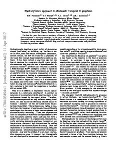
e ε (k, ω) vs. ω for the same level 1 in the column and F IGURE 3. C the parameter values given in Table I.

251

e ε (k, ω), (—–), and F IGURE 4. Comparison between theoretical, C ε experimental ςe (k, ω), (¦) results, and absolute error ∆ (- - -).

TABLE I. Material parameters for an air-water bubble column. z1 ρG ρL µL a ε0 εcp

12.5 cm 1.2046 × 10−3 gr/cm3 0.998 gr/cm3 0.998 gr/cm 0.29 cm 0.0833 0.62

which will be useful to analyze the results obtained in the previous section. e ε (k, ω) as a function of ω and for fixed In Fig. 3 we plot C k = k1 = 2π/z1 , as given by Eq. (62). Here z1 denotes the height of level 1 in the column and we used the parameter values given in Table I. Note that from Eqs. (62)–(65) one verifies that

frequency in Hertz. It should be pointed out that these power spectral densities were further normalized with respect to the value G0 ≡ Gexp (p = 0). ε

exp

A normalized periodgram for ςe (k, ω) ≡ G (p)/G0 is shown in Fig. 2, for an experiment in the homogeneous bubbling regime. It shows that for low frequencies the power spectral density function values are decreasing. The development of further peaks does not contain valuable information since the method to compute the periodgram, through windowing techniques, does not allow to get confidence on these parts of the signal.

5.

Results

To compare our results with experimental measurements of the spectral density of the volume fraction correlation function, we introduce the following dimensionless quantities

e ε (k, ω) ∼ k −4 . C

(68)

This is an interesting result since shows that in spite of the complexity of Eq. (62) as a function of k, an explicit overe ε (k, ω) is obtained which is of the all k dependence for C same type as the one obtained for correlation functions of other complex fluids, such as a liquid crystal in near equilibrium states [36]. e ε (k, ω) and ςe ε (k, ω) vs. ω In Fig. 4 we plot together C for z = z1 . It is apparent that qualitatively, the theory reproduces the decay at low frequencies observed in the experiment. Furthermore, to quantify the differences between both curves for each ω, we introduce the absolute error, ¯ ε ¯ e (z, ω) − ςe ε (z, ω)¯. ∆ ≡ ¯C (69) For the range 0–0.5 Hz, the difference between theory and experiment is larger than in the interval 0.5–1.2 Hz. For the

Rev. Mex. F´ıs. 48 S1 (2002) 243 - 253

252

A. SORIA, E. SALINAS-RODR´IGUEZ, J.M. ZAMORA, AND R.F. RODR´IGUEZ

former ∆ amounts to a percentual difference that varies between 5% for ω = 0.4 Hz and 27% for ω = 0.2 Hz, whereas for the latter interval this difference may be as low as 0.07% for ω = 0.8 Hz and grows up to 11% for ω = 0.5 Hz.

6. Discussion In this work we have introduced a fluctuating hydrodynamic approach to describe some of the properties of a two-phase bubble column. The following comments may be useful to clarify and elaborate on some of our results. It is convenient to emphasize once again, that the hydrodynamic model used in this work [18] is idealized in many aspects. For instance, compressibility and hydrodynamic interactions between bubbles and with the boundaries, have not been taken into account. However, given the complexity of these effects and of the system itself, the simple one dimensional model proposed of Biesheuvel and Gorissen seems to be a good first step in modeling the complex behavior of a bubble column. It also ilustrates how some of the methodology and concepts of kinetic theory and statistical mechanics may be used to deal with complex phenomena in engineering systems. The results obtained with this model show that the agreement between the experimental and theoretical values

∗

. Fellow of SNI.

1. J.B. Joshi, V.P. Utgikar, M.M. Sharma, and V.A. Juvekar, Reviews in Chemical Engineering 3 (1985) 281. 2. Y. Mercadier, Th`esis, Universit´e Scientifique et Medicale et Institut National Polytechnique des Grenoble, France, (1981). 3. J.C. Micaelli, Th`esis, Universit´e Scientifique et Medicale et Institut National Polytechnique des Grenoble, France, (1982). 4. A. Matuszkievicz, J.C. Flamand, and J.A. Bour´e, Int. J. Multiphase Flow 13 (1987) 199. 5. A. Soria and H. De Lasa, Int. J. Multiphase Flow 18 (1992) 943. 6. E. Salinas-Rodr´ıguez, R.F. Rodr´ıguez, A. Soria, and N. Aquino, Int. J. Multiphase Flow 24 (1998) 93.

for the void fraction correlation function is reasonably good with an absolute error which may vary between 0.07%–27%. This fact reinforces the point of view advocated above in the sense that a fluctuating hydrodynamic description of a bubble column may be a useful approach that has not been exploited in engineering systems. We should also mention that in this work we have assumed an initial monodisperse size distribution and the coalescence of bubbles has not been considered. While this assumption has proved to be reasonable, some improvement might be reached if different initial distributions are considered at the upper levels of the bubble column; however, this remains to be assessed.

Acknowledgements One of us (RFR) would like to thank the warm hospitality and support of Area de Ingenier´ıa en Recursos Energ´eticos, Departamento. I.P.H., UAM-I, where this work was done. He also acknowledges partial financial support from grants DGAPA-UNAM, IN101999 and FENOMEC, CONACyT 400316-5-G25427E. AS and ESR, acknowledge partial support from the Instituto Mexicano del Petr´oleo, Mexico, through Grant FIES 97-07-II.

14. D. Ronis, I. Procaccia, and J. Machta, Phys. Rev. A 22 (1980) 714. 15. A.M.S. Tremblay, E.D. Siggia, and M.R. Arai, Phys. Lett. A 76 (1980) 57. 16. J. Machta, I. Oppenheim, and I. Procaccia, Phys. Rev. A 22 (1980) 2809. 17. L.S. Garc´ıa-Col´ın and R.M. Velasco, Phys. Rev. A 12 (1975) 646. 18. A. Biesheuvel and W.C.M. Gorissen, Int. J. Multiphase Flow 16 (1990) 211. 19. L.D. Landau and E.M. Lifshitz, Fluid Mechanics, (Pergamon, 1959).

7. J. Drahos and J. Cermak, Chem. Eng. Process. 26 (1989) 147.

20. R.J.N. Bernier, Ph.D. Thesis, California Institute of Technology, U.S.A., (1982).

8. C.W.M. Van der Geld and C.W.J.Van Koppen, in Measuring Techniques in Gas-liquid Two-Phase Flows, edited by J.M. Delhaye and G. Cognet, (Springer-Verlag, 1984), pp. 525.

21. A. Soria, Ph.D. The University of Western Ontario, London, Canada, (1991).

9. J. March-Leuba, Repport NUREG/CR-6003, ORNL/TM12130 (1992) 10. J. Cerm´ak, F. Kast´anek, and A. Havl´ıcek, Coll. Czech.Chem. Commun. 42 (1979) 56. 11. N. Yutani, N. Ototake, and L.T. Fan, Powder Tech. 48 (1986) 31. 12. N. Yutani, N. Ototake, and L.T. Fan, Ind. Eng. Chem. Res. 26 (1987) 343. 13. N. Yutani, L.T. Fan, and J.R. Too, AIChE J. 29 (1983) 101.

22. G.K. Batchelor, An Introduction to Fluid Dynamics, (Cambridge University Press, 1967). 23. G.K. Batchelor, J. Fluid Mech. 193 (1988) 75. 24. M.J. Lighthill, An Informal Introduction to TheoMolecular Theory of Gases and Liquidsretical Fluid Mechanics, (Oxford University Press, 1986). 25. J.O. Hirschfelder, C.F. Curtiss, and R.B. Bird, (Wiley, 1954). 26. S.A. Rice and P. Gray, The Statistical Mechanics of Simple Liquids, (Wiley, 1965).

Rev. Mex. F´ıs. 48 S1 (2002) 243 - 253

A FLUCTUATING HYDRODYNAMIC APPROACH TO CORRELATION FUNCTIONS IN TWO PHASE BUBBLE COLUMNS

253

27. A. Biesheuvel and S. Spoelstra, Int. J. Multiphase Flow 15 (1989) 911.

32. H.K. Kyt¨omaa and C.E. Brennen, J. Fluid Engng. 110 (1988) 76.

28. G.B. Wallis, One-dimensional Two-phase Flow, (McGraw-Hill, 1969).

33. H.K. Kyt¨omaa and C.E. Brennen, Int. J. Multiphase Flow 17 (1991) 13.

29. L.A. Glasgow, L.E. Erickson, C.H. Lee, and S.A. Patel, Chem. Eng. Commun. 29 (1984) 311. 30. J. Drahos, J. Zahradn´ık, J. Puncoch´ar, M. Fialov´a and F. Bradka, Chem. Eng. Process 29 (1991) 107. 31. A. Tournaire, Th`esis, Universit´e Scientifique et Medicale et Institut National Polytechnique des Grenoble, France, (1987).

34. J.M. Saiz-Jabardo and J.A. Bour´e, Int. J. Multiphase Flow 15 (1989) 483 35. J.C. Maxwell, A Treatise on Electricity and Magnetism I 3rd edition, (Oxford Clarendon Press, 1904). 36. R.F. Rodr´ıguez and J.F. Camacho, Non-equilibrium Effects on the Light Scattering Spectrum of a Nematic Driven by a Pressure Gradient, in this issue.

Rev. Mex. F´ıs. 48 S1 (2002) 243 - 253