A Fluid Approximation for Service Systems Responding to ... - CiteSeerX

Submitted to Operations Research manuscript 2008-09-505.R2, Longer Online Version

06/28/10

A Fluid Approximation for Service Systems Responding to Unexpected Overloads Ohad Perry Centrum Wiskunde & Informatica (CWI), Amsterdam, the Netherlands; [email protected]

Ward Whitt I.E.O.R. Department, Columbia University, New York, NY 10027-6699; [email protected], http://www.columbia.edu/∼ww2040

In Perry and Whitt (2009) we considered two networked service systems, each having its own customers and designated service pool with many agents, where all agents are able to serve the other customers, although they may do so inefficiently. Usually the agents should serve only their own customers, but we want an automatic control that activates serving some of the other customers when an unexpected overload occurs. Assuming that the identity of the class that will experience the overload or the timing and extent of the overload are unknown, we proposed a queue-ratio control with thresholds: When a weighted difference of the queue lengths crosses a pre-specified threshold, with the weight and the threshold depending on the class to be helped, serving the other customers is activated, so that a certain queue ratio is maintained. We then developed a simple deterministic steady-state fluid approximation, based on flow balance, under which this control was shown to be optimal, and we showed how to calculate the control parameters. In this sequel, we focus on the fluid approximation itself, and describe its transient behavior, which depends on a heavy-traffic averaging principle. The new fluid model developed here is an ordinary differential equation driven by the instantaneous steady-state probabilities of a fast-time-scale stochastic process. The AP also provides the basis for an effective Gaussian approximation for the steady-state queue lengths. Effectiveness of the approximations is confirmed by simulation experiments. Key words : large-scale service systems; overload control; many-server queues; fluid approximation; averaging principle; separation of time scales; differential equation; heavy traffic.

1. Introduction History. This paper is an outgrowth of the authors’ first paper on this subject written in 2007. One part was split off and significantly expanded with new material to become Perry and Whitt (2009). This part, introducing and applying the heavy-traffic averaging principle, was revised and submitted to Operations Research in September 2008. Following reviewer reports received in May 2009, a revision was submitted in July 2009. Following a second set of reviewer reports received in May 2010, a version was created for publication in June 2010. This is the remaining longer “unabridged”version to be made available online on the authors’ web pages. After submitting the first version of this paper, the authors completed three new papers on supporting mathematical foundations: Perry and Whitt (2010a,b,c). Responding to unexpected overloads. In Perry and Whitt (2009) we considered how two service systems that normally operate independently, such as call centers, can help each other when one encounters an unexpected overload and is unable to immediately increase its own staffing. We assumed that each service system has a service pool with many agents, each of whom has the ability to serve customers from the other system as well as its own, even though the other customers may be served inefficiently. The goal was to find a way to automatically respond to overloads, without knowledge of the arrival rates, while producing only negligible sharing under normal loads. 1

2

Perry and Whitt: Queue-Ratio Overload Control Article submitted to Operations Research; manuscript no. 2008-09-505.R2, Longer Online Version

Toward that end, we proposed a queue-ratio control with thresholds (QR-T), which activates serving customers from the other system when a weighted difference of the two queue lengths (numbers of waiting customers) exceeds a threshold, allowing sharing in only one direction at any time. There is a target queue-ratio function and threshold for each direction of sharing. The general QR-T control allows the queue ratio to be a function of the two queue lengths, but it often suffices to use fixed queue ratios (FQR-T), which is advantageous because the control then has fewer parameters, namely the two ratio parameters and the two thresholds. These queue-ratio controls are modifications of ones proposed previously in Gurvich and Whitt (2009a,b, 2010). The thresholds and the application to respond to unexpected overloads are new. These QR controls tend to be effective because they simplify the problem by reducing the dimension. With the QR-T control, the two system queues tend to evolve independently when the sharing is not activated (under normal loads), but the two queues tend to evolve together in a fixed relation when the sharing is activated (under overloads). Indeed, under overloads, the two system queues tend to evolve dependently to the maximum extent. This maximum dependence can be formalized by the notion of state-space collapse (SSC), as in Bramson (1998), Dai and Tezcan (2005), Gurvich and Whitt (2009a). The Markovian X model. To analyze this QR-T overload control and determine appropriate control parameters, we considered a Markovian X call-center model, having two customer classes, each with its own queue, and two service pools, each with many agents; see Aksin et al. (2007), Gans et al. (2003), Garnett and Mandelbaum (2000) for background on the basic call-center models. To capture a common motivation for having the systems operate independently under normal loads, we assumed the strong inefficient-sharing condition µ1,1 > µ1,2

and µ2,2 > µ2,1 ,

(1)

where µi,j denotes the service rate of a class-i customer by a type-j agent; i.e., customers tend to get served faster by their own service pool than by the other service pool. However, many of the previous results hold under the weaker basic inefficient-sharing condition µ1,1 µ2,2 ≥ µ1,2 µ2,1 . A fluid model with convex costs. In order to determine appropriate queue-ratio functions and to approximate the performance of this QR-T control, in Perry and Whitt (2009) we introduced a convex-cost framework and a simple deterministic steady-state fluid approximation for the X callcenter model, based on balancing steady-state flow rates. Within that framework, we proved that properly chosen queue-ratio functions minimize the average steady-state cost during an overload incident, without requiring knowledge of the arrival rates. Moreover, we showed how to calculate the optimal queue-ratio functions. In addition, we indicated how to determine the thresholds. We then applied simulation to show that the optimal control for the fluid model is effective for the original stochastic X call-center model. Indeed, the simulations show that the proposed queue-ratio control with thresholds outperforms the optimal fixed partition of the servers given known fixed arrival rates during the overload, even though the proposed control does not use information about the arrival rates. The contributions here. The present paper develops an approximation for the stochastic processes describing the performance of the overloaded X model with the ratio control. The approximation is interesting because it involves a heavy-traffic averaging principle (AP). First, the AP directly yields an approximation for the transient behavior as well as the steady-state behavior. The new approximation for the transient behavior is a deterministic fluid approximation, i.e., an ordinary differential equation (ODE), but it is an unconventional ODE. As a consequence of the AP, the ODE is driven by a function of the ODE state involving the steady-state probability distributions of an associated family of fast-time-scale stochastic processes; see §4. the most familiar example of an AP is no doubt in the theory of nearly-completely-decomposable (NCD) Markov chains, as in Courtois (1977); see Remark 2.4.1 of Whitt (2002) for more discussion and


3

references. We validated the transient approximation based on the ODE by conducting simulation experiments; see §4. We also apply the AP to develop improved approximations for the steady-state distribution. The heuristic steady-state fluid approximation developed in Perry and Whitt (2009) provides only an approximation for the mean queue lengths. First, the AP provides improved approximations for these mean steady-state values; see §6. Effectiveness is confirmed by simulations in §7. Second, the AP provides a tractable approximation for the full steady-state joint distribution of the queue lengths during the overload incident. In particular, the AP leads to a Gaussian approximation, with explicit formulas for the variances; see §8. The full distribution provided by this Gaussian approximation is vital because, for typical system sizes, the standard deviations tend to be roughly of the same order as the mean values. In summary, Perry and Whitt (2009) introduces the overload control problem, the X model and the ratio control, and shows that the control is effective. However, Perry and Whitt (2009) provides only a crude deterministic approximation of steady-state performance, based on rate balance. Here we show how to approximate the full system performance with the control. The Many-Server Heavy-Traffic Regime. The performance of the X model during overloads, including the AP, can be understood by considering the many-server heavy-traffic (MSHT) limiting regime, briefly reviewed here in §2. The overloading puts the large service system in the efficiencydriven (ED) MSHT limiting regime. Experience indicates that in the ED regime we can accurately approximate both the transient and steady-state performance by deterministic fluid models and diffusion-process refinements; e.g., see Garnett et al. (2002), Whitt (2004, 2006). With an understanding of the MSHT ED regime, we can see that an AP is appropriate here. Thus we are able to develop the AP and the associated performance approximations heuristically. We justify these approximations empirically through extensive simulation experiments. In subsequent papers, Perry and Whitt (2010a,b,c), we put the AP and the associated performance approximations on a firm mathematical basis. We show that the ODE stemming from the AP is well defined, with good properties, and that the approximations we develop in this paper arise as MSHT stochastic-process limits involving the AP, paralleling earlier papers by Hunt and Kurtz (1994), Coffman et al. (2005). We prove no limit theorems here. We contribute here by showing that an AP is appropriate in this context and by showing how the SSC and the AP can be applied directly as engineering principles to better understand how large systems perform. In this paper we heuristically develop useful quantitative performance approximations. The rest of the Paper. In §2 we specify the model and review the ED MSHT limiting regime. In §3 we develop the deterministic fluid approximation for the steady-state performance. There are two important cases of unbalanced overloads: (1) when both classes are overloaded after sharing, and (2) when one class is overloaded and the other class remains underloaded even after the sharing. In §4 we develop the deterministic fluid approximation for the transient behavior in the fully-overloaded case; that is a system of ordinary differential equations (ODE’s) based on the AP. In §5 we justify the approximation developed in §4 for the transient behavior of the system during an overload by comparing the predicted performance to simulation results for the transient behavior of the original queueing system using the QR-T control. In §6 we develop two stochastic refinements to the deterministic approximations for the steady-state quantities. In §7 we compare our approximations for steady-state mean values with simulations. In §8 we briefly describe a diffusion approximation to generate normal approximations for the full steady-state distributions. We also compare these normal distribution approximations with simulations. Finally, in §9 we draw conclusions. Additional material appears in an appendix. First, in §EC.1 we present additional comparisons of the normal distribution approximations in §8 with simulations. Next, in §EC.2 we develop an

4


ODE based on the AP to analyze the initially normally-loaded (without an overload) X model operating under FQR without the thresholds, and show that this ODE predicts the bad performance without these modifications previously shown in §4.1 of Perry and Whitt (2009) through simulation. In order to do so, we develop the more complex six-dimensional ODE characterizing the fully overloaded system with two-way sharing and two thresholds. In §EC.3 we continue the discussion begun in §EC.3 of the algorithm developed to describe the bad behavior of ordinary FQR, without any thresholds.In §EC.4 we examine the system under FQR together with one-way sharing, but without thresholds. In §EC.5 we present more detail about the performance of FQR-T under normal loads. In §EC.6 we present additional simulation results, considering asymmetric models and more challenging boundary cases in order to better understand the limitations of the approximations.

2. Preliminaries The model. We now specify the Markovian X model under consideration; it is depicted in Figure 1 of Perry and Whitt (2009). There are two customer classes, with customers from each class arriving according to a Poisson process. There is a queue for each customer class, from which customers are served in order of arrival. We assume that waiting customers have limited patience. A class-i customer will abandon if he does not start service before a random time that is exponentially distributed with mean 1/θi . There are two service pools, with pool j having mj homogeneous servers working in parallel. The service times are mutually independent exponential random variables, but the mean may depend on both the customer class and the service pool. The mean service time for a class-i customer served by a type-j agent is 1/µi,j . As usual, the service times, abandonment times and arrival processes are mutually independent. Let Qi (t) be the number of class-i customers in queue and let Zi,j (t) be the number of type-j agents busy serving class-i customers, at time t. With the assumptions above, the stochastic process {(Qi (t), Zi,j (t); i = 1, 2; j = 1, 2) : t ≥ 0} is a six-dimensional continuous-time Markov chain (CTMC), given any routing policy that depends on the six-dimensional state. We are using this model to describe the system during the overload incident. Our approximation applies after the arrival rates have shifted to new values and after sharing has begun. We assume that customers from the two classes arrive during the overload with constant arrival rates λ1 and λ2 , which make at least one class overloaded. Our goal is to develop approximations for the stochastic process {(Qi (t), Zi,j (t); i = 1, 2; j = 1, 2) : t ≥ 0} during the overload incident. In Perry and Whitt (2009, 2010a) we make a strong case for focusing on the steady-state random quantities Qi ≡ Qi (∞) and Zi,j ≡ Zi,j (∞) in the presence of overloads. First, the abandonment always keeps the system stable, so steady state always exists. Second, steady state tends to be approached relatively quickly; see §EC.1 of Perry and Whitt (2009) for simulation and theoretical support. Thus, we are especially interested in the random vector (Q1 , Q2 ). In this paper we show that (Q1 , Q2 ) can be approximated by a bivariate normal distribution, having correlation 0 without unbalanced overloads (when there is no sharing) and having correlation 1 under unbalanced overloads (when there is sharing). We develop explicit formulas for the means and variances. The FQR-T control. The FQR-T control is based on two nonnegative thresholds k1,2 and k2,1 and two positive queue-ratio parameters r1,2 and r2,1 . We define two (weighted) queue-difference stochastic processes D1,2 (t) ≡ Q1 (t) − r1,2 Q2 (t) and D2,1 (t) ≡ r2,1 Q2 (t) − Q1 (t). As long as D1,2 (t) ≤ k1,2 and D2,1 (t) ≤ k2,1 , we do not allow any sharing, i.e., we only let agents serve customers from their designated class. (Ordinary FQR without thresholds corresponds to r2,1 = r1,2 and k1,2 = k2,1 = 0.) However, pool-2 agents are allowed to start serving class-1 customers when D1,2 (t) > k1,2 , provided that no pool-1 agents are still serving a class-2 customer. (We restrict attention to one-way sharing, i.e., sharing in only one direction at a time, but either direction is possible.) Pool 2 is allowed to begin service as soon as no pool-1 agents are serving class-2 customers and D1,2 (t) > k1,2 .


5

As soon as the first pool-2 agent is assigned to serve a class-1 customer, we drop the threshold k1,2 , but keep the other threshold k2,1 . Thus, once one-way sharing has been activated with pool 2 helping class 1, we use ordinary FQR with ratio parameter r1,2 : Upon service completion, a newly available type-2 agent serves the customer at the head of the class-1 queue (the class-1 customer who has waited the longest) if D1,2 (t) > 0; otherwise the agent serves a customer from his own class. (There also is the other threshold k2,1 , but it will usually not be crossed during the overload incident.) Only one-way sharing in this direction will be allowed until either the class-1 queue becomes empty or the other difference process crosses the other threshold, i.e., when D2,1 (t) > k2,1 . As soon as either of these events occurs, newly available pool-2 agents are only assigned to class 2 and the threshold k1,2 is reinstated. And similarly in the other direction. Even though we intend to drop the threshold k1,2 when sharing is activated with pool 2 helping class 1 (in the manner just described), we consider a centering constant κ1,2 after sharing, which can be interpreted as a threshold. Perry and Whitt (2009) show that in some cases it is actually optimal to use the shifted FQR-T control, i.e., keeping the queues at a fixed ratio centered about a constant. Such is the case, for example, when the holding cost is separable and quadratic, i.e., of the form C(Q1 , Q2 ) = C1 (Q1 ) + C2 (Q2 ), where Ci (Qi ) = ai + bi Qi + ci Q2i ; see §EC.4 in Perry and Whitt (2009). In these cases the optimal relation between the queues is Q1 + r1,2 Q2 = κ1,2 or Q1 + r2,1 Q2 = κ2,1 for some κ1,2 , κ2,1 ∈ R, depending on the direction of sharing; explicit formulas appear in EC.11 and EC.12 of Perry and Whitt (2009). If bi = 0 for i = 1, 2, then the two centering constants take the form κ1,2 = κ2,1 = 0, and we have ordinary FQR once sharing has been activated in some direction. Here we aim to more carefully describe the performance of the system in a single overload incident. The class that is more overloaded will typically change in successive overload incidents. Without loss of generality, we assume that class-1 is the more overloaded class in the overload incident we are considering, so that we focus attention on the single queue-difference stochastic process D1,2 (t) and drop the subscripts on D, r and κ. The ED MSHT limiting regime. We show that the fluid approximations developed here are asymptotically correct in the ED MSHT limiting regime in Perry and Whitt (2010a,b,c), but we do not establish any limits here. Nevertheless, formulating the ED MSHT limiting regime helps to understand how we get the approximations and when they should perform well. The MSHT regimes are specified by considering a sequence of models indexed by n; we let a superscript denote the quantity associated with model n. The main idea is that the system scale should grow. Accordingly, we assume that the arrival rates and number of servers grow proportionally to n: (n) (n) λi ¯ i and mj → m →λ ¯ j as n → ∞, (2) n n ¯ i and m where λ ¯ j are positive constants for i = 1, 2 and j = 1, 2. The individual abandonment-rates θi , and service-rates µi,j remain constant for all n. For a Markovian I model, having one service pool, one customer class and customer abandonment, i.e., the M/M/m + M model, three different MSHT limiting regimes were identified in Garnett et al. (2002): If the system is asymptotically overloaded, then it is called the efficiency-driven (ED) limiting regime; if the system is asymptotically critically loaded, then it is called the quality-andefficiency-driven (QED) limiting regime; if the system is asymptotically underloaded, then it is called the quality-driven (QD) limiting regime. These same cases without abandonment had been specified by Halfin and Whitt (1981). For one class and one pool, it is natural to let n be the total number of( servers) (m ¯ = 1 in (2)). Then the regimes are determined by √ n = n for all n, so that m the limit 1 − ρ(n) n → β as n → ∞, where ρ(n) ≡ λ(n) /nµ is the traffic intensity in model n. The regimes (i) ED, (ii) QED, and (iii) QD then occur, respectively, if the limit holds with (i) β = −∞, (ii) −∞ < β < ∞, and (iii) β = +∞.

6


We will be concentrating on overloaded systems, i.e., the ED regime, which for the I model is discussed in Whitt (2004). That provides important background for our work on the X model here. In that context we will consider the ED regime under the analog of the conventional more restrictive condition that ρ(n) = ρ > 1. With customer abandonment, the ED regime is quite practical because the queue lengths have proper steady-state distributions whenever the abandonment rates are positive. Before the overload occurs, a well-managed large service system will be normally loaded, which usually means that the system will be in either the QD or QED MSHT regime, but then the new arrival rates associated with the overload shift the system into the ED regime. Fluid limits for scaled processes. We now indicate the kind of stochastic-process limits that (n) hold as n → ∞ in the ED MSHT limiting regime specified by (2) with ρi = ρi > 1 for at least one class i (making the system overloaded for at least one class). Our descriptions will be useful when the system remains overloaded for at least one class after the sharing. First, for deterministic fluid limits, we consider the scaled processes (n)

Qi (t) ¯ (n) Q i (t) ≡ n

(n)

Zi,j (t) (n) and Z¯i,j (t) ≡ , n

t ≥ 0.

(3)

These scaled processes converge as n → ∞, with ¯ (n) ¯ (n) ¯ ¯ (Q as i (t), Zi,j (t), i = 1, 2; j = 1, 2) ⇒ (Qi (t), Zi,j (t), i = 1, 2; j = 1, 2)

n → ∞,

(4)

¯ i (t), Z¯i,j (t), i = 1, 2; j = 1, 2) evolves as where ⇒ denotes convergence in distribution and the limit (Q a deterministic dynamical system, in particular, as a six-dimensional ordinary differential equation (ODE) or system of ODE’s. We emphasize that the overloaded ED regime is essential for this limit to be meaningful. In the QD and QED regimes (with appropriate initial conditions) we expect the ¯ i (t) = 0. With FQR-T, we should have minimal sharing when the system is not fluid limit to be Q overloaded, hence we also should have Z¯i,j (t) = 0 for all i, j with i ̸= j and t ≥ 0. The limit in (4) is referred to as a functional weak law of large numbers (FWLLN). From this (n) ¯ i (t) asymptotic perspective, we think of our deterministic fluid approximation as being Qi (t) ≈ nQ (n) ¯ and Zi,j (t) ≈ nZi,j (t). Moreover, we anticipate that all processes have well-defined steady-state limits as t → ∞ and that the double limit in (4) as n → ∞ and t → ∞ (in any order) is valid and equals the limit as t → ∞ of the ODE, which is the unique stationary point for the ODE (but none of that will be proved here). From this asymptotic perspective, we think of our deterministic fluid approximation for the (n) (n) ¯ i (∞) and Zi,j ≡ Zi,j steady-state random variables Qi and Zi,j as being Qi ≡ Qi (∞) ≈ nQ (∞) ≈ ¯ nZi,j (∞) for all suitably large n, but we will not include the n in our heuristic development of the approximations. Refined stochastic limits. Perry and Whitt (2010c) show that there also are associated stochastic limits that serve as refinements of the fluid limits above. For these, we introduce the new scaled processes (n) ¯ i (t) Qi (t) − nQ ˆ (n) √ Q i (t) ≡ n

(n) Zi,j (t) − nZ¯i,j (t) (n) ˆ √ and Zi,j (t) ≡ , n

t ≥ 0.

(5)

These scaled processes also converge as n → ∞, with ˆ (n) ˆ (n) ˆ ˆ (Q as i (t), Zi,j (t), i = 1, 2; j = 1, 2) ⇒ (Qi (t), Zi,j (t), i = 1, 2; j = 1, 2)

n → ∞,

(6)

ˆ i (t), Zî,j (t), i = 1, 2; j = 1, 2) evolves as a stochastic process. The limit in (6) is where the limit (Q referred to as a functional central limit theorem (FCLT).


7

To understand the system steady-state behavior, it suffices to center in (5) by the steady-state ¯ i (∞). Corollary 4.1 of Perry and Whitt (2010c) shows that fluid values, e.g., by subtracting nQ the limit process is essentially a two-dimensional bivariate Ornstein-Uhlenbeck BOU process with ˆ i (t), Zî,j (t), i = 1, 2; j = 1, 2) is a Gaussian process, with zero means, so that the limit process (Q multivariate normal distributions for each t. From this new asymptotic perspective, we think of our stochastic refinement of the fluid approx√ (n) (n) ¯ i (t) + √nQ ˆ i (t) and Zi,j imation as being Qi (t) ≈ nQ (t) ≈ nZ¯i,j (t) + nZî,j (t). From this asymptotic perspective, we think of our refined stochastic approximation for the steady-state √ quantities (n) (n) ¯ i (∞) + √nQ ˆ i (∞) and Zi,j ≡ Zi,j as being Qi ≡ Qi (∞) ≈ nQ (∞) ≈ nZ¯i,j (∞) + nZî,j (∞) for ˆ i (∞), Zî,j (∞); i, j = 1, 2) is a zero-mean some suitably large n, where the stochastic component (Q multivariate normal distribution, which is essentially two-dimensional. Even though we do not do any proofs here, we do verify these properties empirically with simulation. We demonstrate the convergence as n → ∞ in the MSHT limit by showing the performance of the scaled processes for several values of n, in particular, for n = 25, 100 and 400. We see remarkable accuracy for n = 400 and surprisingly good rough approximations even for n = 25. We also see the rapid convergence to steady state as t → ∞. We avoid proofs partly by necessity, because the full story is too long, but also by design: We want to show that these important mathematical ideas – MSHT scaling, SSC and the AP – can be applied directly to establish important engineering results, without providing full mathematical justification. For example, the scaling itself provides very important insights. We use these insights in our fluid analysis of the system, and in choosing the thresholds for sharing. Two time scales. There are two points of view associated with the spatial scaling by n in (3). The first view is that of an inside observer - a customer or an agent. The experience of a customer or an agent is largely independent of n, because the service-time and patience distributions are independent of n. The customer waiting times tend to be independent of n as well. Since the system is overloaded, they converge to positive limits as n → ∞ (unscaled), just as in the M/M/n + M model in the ED regime; see Whitt (2004). The waiting times initially depend on t because we are initially shifting to the new steady state associated with the overload, but they converge to positive deterministic steady-state values as t → ∞. On the other hand, an outside observer has a very different perspective, which changes with n. As the system becomes larger, the time between successive arrivals becomes shorter, as does the time between successive customer abandonments and service completions. Hence, for an outside observer, a larger system means a faster system. Thus, in the same system, there exist different time scales or “clocks:” One clock measures time in units of mean service times and so is of order O(1), while another clock is of order O(1/n), i.e., as the system gets larger, this clock is running faster. When n is large, the faster processes will tend to rapidly approach a local steady-state (in time of order o(1)). We will exploit the different time scales when we construct the fluid approximation. Scaling of the thresholds. As discussed in §6 of Perry and Whitt (2009), the scaling also provides insight into the choice of the thresholds to use to initiate sharing. (We are now not discussing the new centering or shifting constants associated with shifted-FQR.) On the one hand, we want the thresholds large enough that we only rarely initiate sharing inappropriately in response to stochastic fluctuations under normal loading; i.e., we want the thresholds to be large enough to prevent sharing when sharing is not needed. On the other hand, we want the thresholds to be small enough so that we actually succeed in rapidly detecting a genuine overload. There could be a problem, because abandonment alone prevents the queues from reaching high levels. Thus, if the thresholds are too large, then they may never be crossed, even in the presence of overloads. The scaling in the stochastic-process limits provide guidance for the choice of the thresholds. The scaling indicates that we could let the thresholds become smaller, relatively, as n increases, so

8


that they do not have an effect (asymptotically) on the optimal queue ratio; i.e., these thresholds (n) could increase with n, but we should let k1,2 /n → 0 as n → ∞. At the same time, we want these thresholds to be large compared Since the random fluctuations should √ to the stochastic fluctuations. (n) √ be asymptotically of order O( n), we should have k1,2 / n → ∞ as n → ∞. we can simultaneously (n) achieve both objectives if we let the thresholds k1,2 grow like np for 1/2 < p < 1. Then, in the fluid scale, the thresholds are asymptotically negligible, but at the same time these thresholds √ will be large compared to the O( n) stochastic fluctuations. This asymptotic analysis does not tell us what the thresholds should be in any instance, but it suggests that we should be able to find effective thresholds for large systems. We use simulation to choose appropriate thresholds and verify their effectiveness. The extra constants we do consider during the overload incident correspond to shifted-FQR. Clearly, these shifting constants should be of order O(n), so that they appear in the fluid equations. Having these shifting constants be of order O(n) is also revealing in simulations, since it allows us to see the statistical regularity, i.e., the FWLLN. We will see that the scaled performance measures then tend to be independent of n when n is not too small.

3. A Simple Fluid Approximation for the Steady State of the X Model In §5 of Perry and Whitt (2009) we developed a simple deterministic fluid approximation for the steady-state (Qi , Zi,j ; i = 1, 2; j = 1, 2) ≡ (Qi (∞), Zi,j (∞); i = 1, 2; j = 1, 2) of the stochastic process {(Qi (t), Zi,j (t); i = 1, 2; j = 1, 2) : t ≥ 0} under the assumption that the thresholds are dropped after they have been exceeded. A minor modification of the same argument yields corresponding approximations when shifting constants are included after sharing has been initiated (to represent shifted-FQR). We give a brief account here. As before, we do not directly consider the MSHT limiting regime specified in (2), and we do not introduce the scale-factor n, but we are thinking of that regime with a suitably large n. In advance, we do not know which class will experience the overload and need help from the other service pool. Indeed, the direction of sharing may switch in successive overload incidents. However, without loss of generality, when we consider the behavior of the system in one particular overload incident, under an unbalanced overload, we assume that class 1 is overloaded, and more so than class 2 if class 2 is also overloaded. (The precise meaning of “unbalanced overload” and “more so than class 2” is specified in §3.1 below.) Hence, we need only consider the queue-difference process D1,2 (t), now denoted by D(t) ≡ Q1 (t) − rQ2 (t). The overloaded conditions for class 1. When we say that class 1 is overloaded, we mean that λ1 > m1 µ1,1 , which is equivalent to ρ1 ≡ λ1 /(m1 µ1,1 ) > 1, where ρ1 is the class-1 traffic intensity in isolation. In other words, we assume that class 1 with pool 1 alone would produce an M/M/m + M model in the ED regime. Since we have customer abandonment, the system is stable. From §5.1 of Perry and Whitt (2009) or Whitt (2004), we obtain the deterministic fluid approximation for the steady-state queue length of class 1 alone, namely, Qalone ≈ (λ1 − m1 µ1,1 )/θ1 . 1 There are two cases for the less-loaded class 2 after sharing: We may either have class 2 also overloaded, but less so than class 1, or class 2 underloaded. 3.1. The Fully-Overloaded Case: Class 2 Overloaded After Sharing We now describe the conditions for class 2 to be overloaded after sharing, which makes both classes overloaded. First, class 2 might be overloaded alone. Paralleling the analysis above, that occurs if λ2 > m2 µ2,2 or, equivalently, if ρ2 ≡ λ2 /m2 µ2,2 > 1. In that event, the steady-state ≈ (λ2 − m2 µ2,2 )/θ2 . In order to have sharing (class 2 queue length of class 2 alone would be Qalone 2 + κ, where κ here is the shifting constant > rQalone helping class 1) in steady-state, we need Qalone 2 1 associated with shifted FQR-T.


9

Then, for a deterministic fluid model in steady state, there should be approximately a fixed level of sharing, with Z1,2 type-2 agents serving class-1 customers. Thus the queue lengths should be Q1 =

λ1 − (m1 µ1,1 + Z1,2 µ1,2 ) θ1

and Q2 =

λ2 − (m2 − Z1,2 )µ2,2 . θ2

(7)

We now invoke SSC to conclude that we also should have Q1 = rQ2 + κ. (We obtain equality in the fluid model, but only an approximation for the stochastic system.) Then it is easy to see that the desired amount of sharing is the unique solution of the following linear equation in the single variable Z1,2 : ( ) Z1,2 µ2,2 Z1,2 µ1,2 alone alone = rQ2 + κ = r Q2 + + κ. (8) Q1 = Q1 − θ1 θ2 Clearly, there is one and only one value of Z1,2 yielding equality, with D ≡ Q1 − rQ2 = κ, because at Z1,2 = 0 the left side is greater than the right side, by assumption, and the left (right) side is decreasing (increasing) in Z1,2 , so that there must be equality for one and only one value of Z1,2 . If the solution yields Z1,2 > m2 , then the required sharing is not possible. In that event, even if all class 2 agents work on class-1 customers, the overloads can not be balanced in the desired way. However, if 0 ≤ Z1,2 ≤ m2 , then we have found our desired answer. All three variables Q1 , Q2 and Z1,2 can equivalently be found by solving the following two equations in two unknowns (Q1 and Z1,2 ): λ1 − (m1 µ1,1 + Z1,2 µ1,2 ) Q1 − κ λ2 − (m2 − Z1,2 )µ2,2 Q1 = and Q2 = = . (9) θ1 r θ2 The fluid equations in Perry and Whitt (2009) arise when we set κ = 0 in (9). Now suppose that class 2 alone is underloaded. We now consider the common case in which class 2 is initially underloaded, but becomes overloaded when it helps class 1. It is easy to see that this case is also covered by the pair of equations in (9). The equations for Qi can be interpreted as balancing the rate in with the rate out, assuming a fixed positive queue length for that class. The only requirement of the solution to (9) is that 0 ≤ Z1,2 ≤ m2 and Q2 ≥ 0. We will then necessarily have Q1 = rQ2 + κ. Example 1. (canonical example) A canonical (symmetric) example for FQR-T has λi = 90, mi = 100, θi = 0.2, µi,j = 1 for all i and j, r = 1 and thresholds k1,2 = k2,1 = 10 before the overload incident, but then a shift to λ1 = 130 under an unexpected overload for class 1. The simple fluid approximations above yield Q1 ≈ 150 and Q2 ≈ 0 if we assume that there is no sharing after the overload, and then Q1 ≈ Q2 ≈ 50 using simple FQR (no shift. κ = 0) after sharing. The associated approximate potential waiting times (expressed in mean service times) for class 1 are reduced from 1.5 to 0.5 at the expense of increasing class-2 waiting times from 0 to 0.5. (When the holding costs are convex, such a tradeoff may be beneficial.) Simulation shows that this is indeed what happens, approximately. 3.2. The Spare-Capacity Case: Class 2 Underloaded After Sharing The remaining case is the fortunate case when the class-2 load is low when the class-1 load is unexpectedly high. Then pool 2 might be able to help class 1 without penalty. Clearly, the FQR-T control is very desirable in this case. From the fluid model perspective (ignoring stochastic fluctuations), this case occurs if and only if we can simultaneously have Q1 = κ and Q2 = 0. Assuming that there always are available agents in pool 2, a type-2 agent immediately serves a class-1 customer, whenever an arriving customer finds κ customers in queue 1. Hence, we must have Q1 (t) ≤ κ. In the fluid model, we achieve that

10


value κ for Q1 if and only if Z1,2 serves to balance the rate in and rate out at queue 1. Since the rate into queue 1 is λ1 , while the rate out is m1 µ1,1 + κθ1 + Z1,2 µ1,2 , we obtain Z1,2 =

λ1 − m1 µ1,1 − κθ1 , µ1,2

(10)

while still allowing queue 2 to be empty; i.e., so that the rate into queue 2 is λ2 , which is less than or equal to the maximum rate out of queue 2, which is µ2,2 (m2 − Z1,2 ). Consequently, we still have Q2 = 0 along with Q1 = κ. We necessarily have Z1,2 < m2 .

4. The Fluid-Model System of ODE’s in the Fully Overloaded Case We will now introduce the deterministic fluid-model ODE’s to approximate the transient behavior of the CTMC {(Qi (t), Zi,j (t); i = 1, 2; j = 1, 2) : t ≥ 0} in the fully overloaded case considered in §3.1. From an asymptotic perspective, we think of this approximation as stemming from the FWLLN (4), but we develop the approximation directly, without considering a sequence of models. (See Perry and Whitt (2010a,b,c) for the associated supporting asymptotic results.) We start when the overload begins, at the instant the arrival rates change. The ODE’s should apply to all possible initial conditions, but the standard case is for the system to be initially in steady state with the two service pools operating independently at normal levels. The sudden shift in the arrival rates causes the system to go through two transient periods. In the first transient period, the two systems continue to operate independently, with each responding to its own new arrival rate. In the fully overloaded case being considered, the first transient period ends and the second transient period begins after D(t) exceeds its threshold and sharing is initiated, with all servers in both pools busy. That is when the AP begins to operate. The system evolves in this second transient period approaching the steady state associated with the overload. It is this new steady state, in overload, that we are primarily trying to describe. In this section we are focusing on the second transient period. (See §8 of Perry and Whitt (2010a) for discussion of the first transient period.) 4.1. A Heavy-Traffic Averaging Principle In §3.1 we exploited SSC to deduce the steady-state relation Q1 = rQ2 + κ in the fully-overloaded case (using shifted FQR with centering constant κ), with pool 2 serving some of the class-1 customers. However, it is evident that SSC does not actually occur in such a simple way. Instead, the queue-difference process D(t) ≡ Q1 (t) − rQ2 (t) oscillates around the centering constant κ. The key observation is that the queue-difference process D(t) moves back and forth across the boundary κ relatively quickly, because it has a strong drift pointing toward κ on both sides (under typical overload conditions). These boundary crossings occur in a faster time scale than the relative changes in the other processes under consideration. All processes move due to the same arrivals and service completions (which are happening quickly because of the scale), but the processes Qi (t) and Zi,j (t) tend to be large, of the same order as the number of servers, which we assume is itself large, e.g., 100. In a very small amount of time, the fluid processes Qi (t) and Zi,j (t) do not change much relative to their values, while D(t) moves rapidly between the two regions (−∞, κ) and [κ, ∞). Since the process D(t) moves back and forth across its boundary κ rapidly, we conclude that D(t) approximately reaches a time-dependent steady state instantaneously at each time t, where that steady-state distribution depends on the time-dependent quantities Qi (t) and Zi,j (t). Let Dt (∞) denote a random variable with that time-dependent steady-state distribution. We will then exploit the time-dependent probabilities π1,2 (X(t)) ≡ P (Dt (∞) ≥ κ). To obtain the steady-state quantity Dt (∞), we introduce a new stochastic process Dt ≡ {Dt (s) : s ≥ 0}, which is the process {D(t + s) : s ≥ 0}, initialized at D(t), but with the transition rates of the stochastic process D, under the extra condition that (Q1 , Q2 , Z1,2 ) remain fixed at their values at time t.


11

This AP allows us to regard Dt approximately as a pure-jump continuous-time Markov process (MP), with state space {k + rj : k ∈ Z, j ∈ Z}. with transition rates that depend only on the fluidmodel state at time t. There are four possible transitions in each state: ±1 and ±r. We obtain simplification without practical sacrifice by assuming that r is rational. For rational r ≡ j/k, this is a CTMC on the state space {j/k : j ∈ Z}. We multiply by k to make all the states integers. Moreover, then the CTMC can be represented as a homogeneous quasi-birth-and-death (QBD) process, as in Definition 1.3.1 and §6.4 of Latouche and Ramaswami (1999). For each t, we can apply the logarithmic reduction algorithm in §8.7 of Latouche and Ramaswami (1999) to efficiently calculate the steady-state distribution of Dt , i.e., the distribution of Dt (∞). As a consequence, we can calculate the desired probabilities π1,2 (X(t)), given any state vector X(t) ≡ (Q1 (t), Q2 (t), Z1,2 (t)). We now specify the transition rates of the CTMC Dt given the time t and the state X(t), using the (j) (k) (j) (k) integer state space. Let λ+ (m, X(t)), λ+ (m, X(t)), µ+ (m, X(t)) and µ+ (m, X(t)) be the transition rates of the FTSMC Dt for transitions of +j, +k, −j and −k, respectively, when Dt (s) = m > κ. (j) (k) (j) Similarly, we define the transitions when Dt (s) = m ≤ κ: λ− (m, X(t)), λ− (m, X(t)), µ− (m, X(t)) (k) and µ− (m, X(t)). First, for Dt (s) = m ∈ (−∞, κ], the upward rates are (k)

λ− (m, X(t)) = λ1 ,

(j)

and λ− (m, X(t)) = µ1,2 Z1,2 (t) + µ2,2 Z2,2 (t) + θ2 Q2 (t),

(11)

corresponding, first, to a class-1 arrival and, second, to a departure from the class-2 queue, caused by a type-2 agent service completion (of either customer type) or by a class-2 customer abandonment. Similarly, the downward rates are (k)

(j)

µ− (m, X(t)) = µ1,1 Z1,1 (t) + θ1 Q1 (t) and µ− (m, X(t)) = λ2 ,

(12)

corresponding, first, to a departure from the class-1 customer queue, caused by a class-1 agent service completion or by a class-1 customer abandonment, and, second, to a class-2 arrival. Next, for Dt (s) = m ∈ (κ, ∞), we have upward rates (k)

λ+ (m, X(t)) = λ1

(j)

and λ+ (m, X(t)) = θ2 Q2 (t),

(13)

corresponding, first, to a class-1 arrival and, second, to a departure from the class-2 customer queue caused by a class-2 customer abandonment. The downward rates are (k)

µ+ (m, X(t)) = µ1,1 Z1,1 (t) + µ1,2 Z1,2 (t) + µ2,2 Z2,2 (t) + θ1 Q1 (t)

(j)

and µ+ (m, X(t)) = λ2 ,

(14)

corresponding, first, to a departure from the class-1 customer queue, caused by (i) a type-1 agent service completion, (ii) a type-2 agent service completion (of either customer type), or (iii) by a class-1 customer abandonment and, second, to a class-2 arrival. We conclude the definition of the FTSP by noting that great simplification occurs in the special case r = 1, because then the CTMC reduces to a simple birth-death (BD) process instead of a QBD process. Then it is easy to calculate π1,2 (X(t)); e.g., see Theorem 5.1 of Perry and Whitt (2010c). 4.2. The ODE In the previous subsection, we observed that the rate of change of the fast-time-scale queue difference process Dt depends on (i) the state X(t) and (ii) whether or not Dt (s) > κ. In the same way, the rates of the CTMC X at time t depend on (i) X(t) itself and (ii) the state of D(t). Now, for the deterministic fluid approximation of the evolution of X(t), we let the rates (derivatives) depend on (i) X(t) itself and (ii) the steady-state probability π1,2 (X(t)) = P (Dt (∞) > κ). First, given Zi,j (t) and πi,j (X(t)), we obtain ODE’s for the two queue-length processes. Let x˙ ≡ x(t) ˙ denote the derivative of x evaluated at t. We let the derivative Q˙ 1 (t) equal the rate

12


of increase of Q1 (t) minus its rate of decrease. The rate of increase is simply the arrival rate to customer queue 1, λ1 . The rate of decrease is more complicated. First, there is the rate of abandonment from queue 1, which is Q1 (t)θ1 . Second, there is the rate of decrease from queue 1 due to service completions by servers who will next take customers from queue 1, which depends on the state of the queue-difference stochastic process. Exploiting the AP, we will not focus on the actual state of the queue-difference process, but instead focus on the average state, assuming that the queue-difference process oscillates relatively rapidly compared to the other processes. We thus assume that a proportion π1,2 (X(t)) of the time that the queue-difference exceeds the shifting constant κ. That portion of the decrease rate is π1,2 (X(t)) (Z1,2 (t)µ1,2 + Z2,2 (t)µ2,2 ). There will be corresponding, but different, rates of decrease for the proportion of time 1 − π1,2 (X(t)) that the queue-difference is less than or equal to κ. That reasoning leads to the system of three ODE’s Q˙ 1 (t) ≡ λ1 − m1 µ1,1 − π1,2 (X(t)) [Z1,2 (t)µ1,2 + Z2,2 (t)µ2,2 ] − θ1 Q1 (t) Q˙ 2 (t) ≡ λ2 − (1 − π1,2 (X(t))) [Z2,2 (t)µ2,2 + Z1,2 (t)µ1,2 ] − θ2 Q2 (t)

(15)

Z˙ 1,2 (t) ≡ π1,2 (X(t))Z2,2 (t)µ2,2 − (1 − π1,2 (X(t)))Z1,2 (t)µ1,2 , ˙ More compactly, we have a single three-dimensional ODE with the general form X(t) = Ψ(X(t), t) for a function Ψ. In addition, our ODE is autonomous (or time invariant) because Ψ(X(t), t) ≡ Ψ(X(t)). An autonomous ODE does not depend explicitly on the time-argument t, and its behavior is invariant to shifts in the time origin. Thus we propose the autonomous ODE ˙ X(t) ≡ (Q˙ 1 (t), Q˙ 2 (t), Z˙ 1,2 (t)) = Ψ(X(t)) ≡ Ψ(Q1 (t), Q2 (t), Z1,2 (t)),

t ≥ 0,

(16)

where Ψ : [0, ∞)2 × [0, m2 ] → R3 is displayed via (15) above. The derivatives in (15) are evident given the transition rates of the CTMC, given that we replace the CTMC by an ODE and invoke the AP. In summary, we can apply standard iterative algorithms for solving ODE’s to solve the ODE (16), where we calculate π1,2 (X(t)) at each step. We used the classical forward Euler algorithm for the ODE together with the logarithmic reduction algorithm for QBD’s from Latouche and Ramaswami (1999); additional details are provided in §5 and §9 of Perry and Whitt (2010a). Steady state. We now characterize the steady state of the fluid model in the fully overloaded case with one-way sharing. We can directly apply the ODE for Z1,2 (t) to find π1,2 by noting again that in steady state Z˙ 1,2 (t) = 0. Thus, π1,2 =

Z1,2 µ1,2 . Z1,2 µ1,2 + (m2 − Z1,2 )µ2,2

(17)

This yields (9). In §6.1 we show how to use the AP to refine the fluid equations (9).

5. Validating the Transient Approximation through Simulation Experiments We now want to provide evidence that our proposed approximation is effective for the transient behavior. Accordingly, in this section we compare numerical results for the transient behavior of the fluid model, based on our algorithm from Perry and Whitt (2010a), to simulation estimates of the actual performance measures in the original queueing model. This will show that the transient approximations are computable and sufficiently accurate for engineering applications. We will show that the deterministic fluid model does not capture important stochastic fluctuations unless the scale is very large, but the fluid model provides remarkably accurate approximations for the mean values of the key queueing processes, Q1 (t), Q2 (t) and Z1,2 (t), provided that the scale is not too small.


13

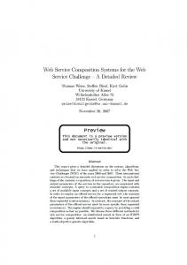
In order to demonstrate the MSHT limits in the ED regime described in §2, we report results for scaled processes, as in (3), for several values of n. We will then be confirming the FWLLN in (4) via the simulation. Our simulation examples throughout the paper will have parameters related to a base case that we consider here as well. It has several parameters depending on (n) (n) (n) n: mi ≡ mi = n, λ1 ≡ λ1 = 1.3n, λ2 ≡ λ2 = 0.9n and κ ≡ κ(n) . Here we take κn = 0, but we will later also consider a positive κ, specifically κ ≡ κn = 0.1n. The other model parameters are independent of n: θ1 = θ2 = 0.2, µ1,1 = µ2,2 = 1.0 and µ1,2 = µ2,1 = 0.8. The arrival rates are chosen to put class 1 in a focused overload, while class 2 is initially normally loaded or slightly underloaded, but becomes overloaded too after the sharing. The rest of the parameters are chosen to make a symmetric model, where serving the other class is less efficient. We use the FQR-T control with ratio parameter r = 0.8; this makes the QBD matrices be as in (23) and (24) of Perry and Whitt (2010a), following the general structure in Section 4.2 there; the algorithm is given in §9.3 there. We have in mind large-scale applications, e.g., with n ≥ 50, but to test the limits of the approximations, we also consider smaller systems. Specifically, we consider the three cases: n = 10, n = 25 and n = 100, initialized empty. Since the processes are scaled, they all have the same fluid approximation. For each n, we ran 1000 independent replications, sampling each of the 1000 simulated sample paths every h ≡ 0.01 time units over the time interval [0, T ] = [0, 50]. This gives 5001 sample points for each replication. Figures 1-3 show the fluid approximation together with simulation estimates of the timedependent mean values for each n, specifically, the averages of the 1000 observed values of three (n) (n) −1 (n) ¯ (n) scaled processes Q Qi (t), i = 1, 2, and Z¯1,2 (t) ≡ n−1 Z1,2 (t) at each of the 5001 sample i (t) ≡ n ¯ (n) points. Figure 4 shows one sample path of {Q 1 (t) : 0 ≤ t ≤ 50}, when n = 100, together with the fluid approximation, to show the typical stochastic fluctuations. These stochastic fluctuations are the reason for using a large number of replications in order to accurately estimate the mean values at each point along the sample path. The statistical precision of the estimators is directly visible in the plots, because the processes are effectively in steady state in the second half of the time interval √ [0, 50]. As n grows larger, the impact of these fluctuations decreases; they are of order 1/ n by (6). The stochastic fluctuations show the importance of the diffusion refinements in §8. Consistent with the FWLLN in (4), the larger the system, the better the fluid approximates the means. The figures clearly show that n ≥ 100 is “large enough,” in the sense that the simulated means are extremely close to the fluid approximation. Even a relatively small system, with only 25 agents in each pool, is approximated quite well by the fluid. However, the fluid approximation is quite rough when n = 10. There is approximately 25% difference between the fluid and the means ¯ (n) of Q 2 (t) when n = 10. Nevertheless, the fluid approximation is useful even for small systems, because the shape of the curves of the simulation means for n = 10 is the same as the shape of the fluid curve; in particular, the rate of convergence to steady state is about the same in all systems. Since the fluid approximation was shown to converge exponentially fast to steady state in §7.3 of Perry and Whitt (2010a), we see that the same must be true, approximately, for the queueing system even for quite small numbers of servers.

6. Stochastic Refinements to the Steady-State Fluid Approximation In this section we present two stochastic refinements to the deterministic fluid-model approximations for the steady-state quantities Qi and Z1,2 describing performance during the overload, assuming shifted FQR is used then. The first exploits the AP to determine the average queue difference for the fully-overloaded case in §3.1. The second develops a birth-and-death-process (BD) approximation for the steady-state queue length Q1 in the spare-capacity case of §3.2.


14

Means and Fluid of Scaled Q1

Means and Fluid of Scaled Q2

0.7

0.9 0.8 Scaled Time−Dependent Values

Scaled Time−Dependent Values

0.6

0.5

0.4

0.3

0.2 n=10 n=100 n=25 fluid

0.1

0 0

10

20

30

40

0.7 0.6 0.5 0.4 0.3 n=10 n=25 n=100 fluid

0.2 0.1 0 0

50

10

20

Time

Figure 1

30

40

50

Time

A comparison of simulation estimates ¯ (n) (t)] for n = 10, 25, 100 to the of E[Q 1 fluid approximation in the base case.

Figure 2

A comparison of simulation estimates ¯ (n) (t)] for n = 10, 25, 100 to the of E[Q 2 fluid approximation in the base case.

One Sample Path and the Fluid of Scaled Q1

Means and Fluid of Scaled Z12 0.35

0.9 0.8 0.7

0.25

Scaled Queue Length

Scaled Time−Dependent Values

0.3

0.2

0.15

0.1 n=10 n=25 n=100 fluid

0.05

0 0

10

20

30

40

0.6 0.5 0.4 0.3 0.2 simulation fluid

0.1 0 0

50

10

Time

Figure 3

20

30

40

50

Time

A comparison of simulation estimates (n) of E[Z¯1,2 (t)] for n = 10, 25, 100 to the fluid approximation in the base case.

Figure 4

A comparison of one sample path of ¯ (n) (t) when n = 100 to the fluid Q 1 approximation in the base case.

6.1. The Average Difference E[D] in the Fully-Overloaded Case We have observed that SSC does not happen exactly; we do not get precisely Q1 (t) = rQ2 (t) + κ. Instead, under the overloading we are considering, the queue-difference process D(t) oscillates around the centering constant κ. As discussed in §4.1 above, we can apply the AP to find an approximating steady-state distribution of D(t) by treating it as a fast-time-scale Markov process (MP). Let D denote a random variable with the limit of these steady-state distributions as t → ∞. We propose refining our fluid approximation for the steady-state distribution by replacing the target difference κ by the mean E[D]. To find E[D] we solve the balance equations of the FTSP above, and then take the mean ∞ ∑ E[D] = jP (D = j). (18) j=−∞

Since the drifts tend to point strongly toward the centering constant κ, it usually suffices to perform the sum for κ − 20 ≤ j ≤ κ + 20. We now obtain our refined approximation, assuming that the queue difference is E[D] instead of κ. The calculation of E[D] can be easily done if Q1 , Q2 and Z1,2 are known. Since they depend


15

on the value E[D], we need to solve for them simultaneously. To do that, we propose an iterative algorithm which solves the three equations λ1 − (m1 µ1,1 + Z1,2 µ1,2 ) , θ1 ∞ ∑ E[D] = jP (D = j). Q1 =

Q2 =

Q1 − E[D] λ2 − (m2 − Z1,2 )µ2,2 = , r θ2 (19)

j=−k2,1

For the iterative procedure, it is natural to start with the values of Q1 , Q2 and Z1,2 obtained from (9), and then calculate the distribution of D and E[D]. We can then obtain new values of Q1 , Q2 and Z1,2 by solving (9) again with E[D] replacing κ. We then can keep iterating. Experience indicates that this iteration consistently converges in a few iterations (typically only two), yielding the solution to (19). 6.2. A BD-Process Refinement for the Spare-Capacity Case For the case in which queue 2 has spare capacity, considered in §3.2, we now develop another refinement, obtaining a non-degenerate approximation for the distribution of Q1 . In this case, because of the available agents in pool 2, as soon as Q1 exceeds the centering constant κ, an idle pool-2 agent serves a customer from class 1. Thus, it is evident that we must have Q1 ≤ κ. Because of the averaging principle, it is not hard to estimate the approximate distribution of Q1 . To do so, we observe that we can regard the class-1 queue as evolving below the level κ1,2 by itself as a BD process. When the queue length is j, the birth rate is a constant λ1 , while the death rate is approximately m1 µ1,1 + θ1 j. (Queue 2 plays no role.) For the reason given, the birth rate is 0 when the queue is at κ. The death rate should be small when the queue length is small. For the approximation to be good, we do not want Q1 to spend much time at very low levels, like 1 or 0. That can be verified approximately by looking at the approximate BD steady-state distribution. In any case, we let the death rate be 0 when the queue length is 0. Our refined approximation for the distribution of Q1 is the steady-state distribution of this finite-state BD process. Since Qalone = (λ1 − m1 µ1,1 )/θ1 > κ, the birth rate always exceeds the death rate here. Indeed, 1 the BD process here for κ − Q1 (t) is stochastically bounded above by the queue-length process in an M/M/1/κ queue, where κ serves as the size of a finite waiting room. If we take the asymptotic perspective in §2, this stochastic bound shows that the difference κ − Q1 should be of order O(1) as √ n → ∞. Hence this adjustment should be asymptotically negligible in both the diffusion scale ( n) and the fluid scale (n). However, the refinement can help in actual examples, even large ones with 1000 servers in each pool. As a refined deterministic fluid approximation, we use the mean value of the steady-state distribution of the BD process here. However, by this method, we also obtain an estimate for the variance and the entire distribution of Q1 . The observed M/M/1 structure indicates that the distribution of κ − Q1 (t) should be approximately a truncated geometric distribution. That is quite different from the approximate normal distribution we derive for the fully-overloaded case in §8.

7. Simulation Experiments to Evaluate the Steady-State Mean Values The overloaded case. We have developed deterministic fluid approximations for the steady-state mean values in the fully overloaded case via the solutions to the two equations in (9) and the three equations in (19). We now compare these approximations to simulation estimates. In order to use the simulation to substantiate the conjectured stochastic-process limits in §2, we choose parameters corresponding to scaled systems, indexed by n, letting n take the values 25, 100 and 400. We have considered much larger n, such as n = 1000, but from the results for n = 400, we see that accurate results will be obtained for all n larger than 400.


16

We consider the base case, introduced in §5, with r = 1. This makes the model symmetric and reduces the fast-scale MP to a BD process. In the Appendix we present corresponding results for asymmetric models. In all our simulation experiments, we used 5 independent runs, each with 300, 000 arrivals. We report averages together with the half widths of the 95% confidence intervals, based on a t statistic with four degrees of freedom. Simulation results for the base case above are presented in Table 1 below. Table 1 shows both the steady-state mean values and the associated scaled values (i.e.,

perf. meas. E[Q1 ]

n=25 2 equ. 3 equ. 16.6 14.4

n=100 2 equ. 3 equ. 65.6 63.1

E[Q1 /n]

0.656

0.656

E[Q2 ]

13.6

E[Q2 /n]

0.556

E[D]

−

κ − E[D]

−

E[Z1,2 ]

5.3

E[Z1,2 /n]

0.211

sim. 15.7 ±0.3 0.575 0.629 ±0.013 16.4 15.9 ±0.4 0.656 0.636 ±0.016 −2.0 −0.2 ±0.3 5.0 3.2 ±0.3 5.8 5.6 ±0.1 0.231 0.224 ±0.003

55.6 0.556 − −

21.1 0.211

sim. 63.6 ±1.9 0.631 0.636 ±0.019 58.6 58.6 ±1.8 0.586 0.586 ±0.018 4.6 5.0 ±0.1 5.4 5.0 ±0.1 21.7 21.9 ±0.04 0.217 0.219 ±0.004

n=400 2 equ. 3 equ. sim 262.2 259.7 258.3 ±5.0 0.656 0.649 0.646 ±0.013 222.2 225.3 223.9 ±5.0 0.556 0.563 0.560 ±0.013 − 34.4 34.4 ±0.04 − 5.6 5.6 ±0.04 84.4 85.1 84.2 ±1.2 0.211 0.213 0.210 ±0.003

Table 1 A comparison of the basic fluid approximations based on two equations in (9) and its refinement based on the three equations in (19) with simulation results in the base case, having m1 = m2 = 1.0n, λ1 = 1.3n, λ2 = 0.9n, µ1,1 = µ2,2 = 1.0, µ1,2 = µ2,1 = 0.8, θ1 = θ2 = 0.2 and κ = 0.1n (rounding up to the nearest integer if necessary).

divided by n). The unscaled values helps us evaluate the performance of the actual system, while the scaled values show the convergence of the stochastic-process limits in (4). Table 1 clearly shows that the level of accuracy grows as n gets larger, but even for relatively small systems, the fluid approximation gives reasonable results. Table 1 also gives the approximation for the steady-state mean of the unscaled weighteddifference process D(t), as developed in §6.1, and compares it to simulation results. The sixth row in the table is especially insightful. It shows that E[D] is about the same distance from κ1,2 for each n, thus strengthening our claim that D(t) should have fluctuations of order O(1) as n → ∞. In closing, we remark that we rounded up the centering constant κ to the nearest integer when n = 25; i.e., we used κ = 3 when n = 25. In the table we show the fluid solution using κ = 2.5 so as to make the scaled fluid solutions uniform. However, the solution using κ = 3 is similar. Independent Cases. One of our objectives is to avoid sharing without unbalanced overloads. That occurs in two scenarios: (i) under normal loads, and (ii) under balanced overloads. In both of these cases our FQR-T control makes the X model operate approximately as two independent M/M/n + M systems, each operating in the QD or QED regime in the first scenario (depending on the actual load of each queue), or the ED regime in the second scenario. We present supporting simulation results in the Appendix.


17

The spare-capacity case. For the spare capacity case, we modify the base case above to make queue-1 overloaded, while pool-2 has enough spare capacity to potentially serve all the extra class-1 customers. As before, we just change the arrival rates, in this case to λ1 = 1.1n and λ2 = 0.8n. It is easy to see that pool 2 has spare capacity (in the fluid scale). We can analyze the available capacity from this deterministic-fluid-approximation perspective as follows: First, we observe that class 1 has an extra arrival rate of 0.1n, whereas pool 2 has 0.2n “extra” service rate, assuming that 0.8n servers are enough to take care of all the class-2 arrivals. Since pool-2 agents serve class-1 customers at rate µ1,2 = 0.8, we initially estimate that we need to have at least 0.125n pool-2 agents working with class-1 customers. However, upon further analysis, we see that the number of pool-1 agents needed is actually less than that, because queue 1 will stabilize at the centering constant κ = 0.1n, and thus θ1 Q1 = 0.02n class-1 customers will abandon. Hence, only about 0.105n pool-2 agents should be needed to serve class 1. In any case, pool 2 has spare capacity. We compare the approximation from §3.2 with simulation results in Table 2. The approximations are given in §3.2. Our initial approximation for Q1 from §3.2 is κ, but that is not shown in Table 2. Instead, we only show the BD refinement from §6.2. (The cruder approximation would yield values of 2.5, 10.0 and 40.0 in the first row.) We see that the refined approximation is much better for large n. For the approximation of Z1,2 , we use (10).

perf. meas. E[Q1 ] E[Q1 /n] E[Q2 ] E[Q2 /n] E[Z1,2 ] E[Z1,2 /n] Table 2

n=25 approx. sim. 1.1 3.3 ±0.1 0.04 0.13 ±0.00 0 3.4 ±0.05 0 0.14 ±0.00 2.5 3.9 ±0.1 0.100 0.156 ±0.007

n=100 approx. sim. 5.2 6.4 ±0.6 0.05 0.06 ±0.01 0 2.7 ±0.5 0 0.027 ±0.005 10.0 12.2 ±0.5 0.100 0.122 ±0.007

n=400 approx. sim. 29.0 30.1 ±0.5 0.07 0.07 ±0.00 0 1.0 ±0.2 0 0.003 ±0.000 40.0 43.4 ±1.2 0.100 0.108 ±0.003

A comparison of the approximation for the steady-state performance measures in the spare-capacity case with simulation results. The arrival rates are now λ1 = 1.1n and λ2 = 0.8n.

8. A Diffusion-Process Refinement In the fully-overloaded case, we now go beyond the deterministic fluid approximation to obtain a diffusion-process refinement, which yields a non-degenerate approximation for the steady-state distribution of the two queue lengths. The approximating distribution is bivariate normal, where the means are the previous fluid approximations. In addition, the approximating correlation is 1 and the variances are V ar(Q1 ) ≈

r2 (λ1 + λ2 ) (1 + r)(rθ1 + θ2 )

and V ar(Q2 ) ≈

(λ1 + λ2 ) . (1 + r)(rθ1 + θ2 )

(20)

A special case. We base our approximation on a special case for which we can easily do the asymptotic analysis exactly, and then we extend the approximation heuristically to other cases. The

18


special case has θ1 = θ2 and µ1,2 = µ2,2 (with class 1 overloaded as usual). Under those additional assumptions, the total queue length Qs (t) ≡ Q1 (t) + Q2 (t) behaves the same as the queue length in the M/M/m + M model in the ED regime, as analyzed in Whitt (2004). In this special case, we can directly obtain a FCLT like (6) for the total queue-length stochastic process, centered about the steady-state fluid limit. From Whitt (2004), we see that the limit is an Ornstein-Uhlenbeck diffusion process with infinitesimal mean m(x) = −θ1 x and infinitesimal variance σ 2 ≡ σ 2 (x) = 2(λ1 + λ2 ). That diffusion process has a normal steady-state distribution. We invoke SSC to treat the individual queue lengths; that yields the correlation 1. Here are additional details: Since the system is fully overloaded, as an approximation we assume that all the agents are busy all the time. (That is asymptotically correct in the MSHT limit.) Thus, the departure rate by service completion has the constant value m1 µ1,1 + m2 µ2,2 . The assumption that µ1,2 = µ2,2 implies that it does not matter which class the type-2 agents are serving. Since the total arrival process is a superposition of two independent Poisson processes, the total arrival process is directly a Poisson process with rate λ1 + λ2 . Finally, since θ1 = θ2 , there is a common abandonment rate for both classes. A heuristic refinement. Now we heuristically extend this same tractable OU approximation with a normal steady-state distribution to more general cases. First, when µ1,2 ̸= µ2,2 , we again act as if all agents are busy all the time. The total service rate at time t is then m1 µ1,1 + Z1,2 (t)µ1,2 + (m2 − Z1,2 (t))µ2,2 . To obtain the desired constant rate, we act as if Z1,2 (t) is constant, assuming its determined deterministic steady-state fluid approximation. This is a heuristic approximation, because we are ignoring the stochastic fluctuations in Z1,2 . Experiments show that this simple approximation works pretty well, but as n → ∞ in the ED regime the infinitesimal mean of the scaled queue-length process does in fact depend on the stochastic behavior of the scaled version of the stochastic process Z1,2 (as we would expect); i.e., simulations show that this heuristic extension is not asymptotically correct as n → ∞, but it is a useful approximation, because it is easier to calculate and the error tends to be small. We also treat the abandonments in a similar way when θ1 ̸= θ2 . We will approximate by a constant abandonment rate applying to all customers. For this step we also will invoke SSC (ignoring the difference), and assume that Q1 (t) ≈ rQs (t)/(1 + r) (and similarly for Q2 ). Thus our approximating constant abandonment rate to apply to the total queue length is θ ≈ (rθ1 /(1 + r)) + (θ2 /(1 + r)). With the new approximating total service rate and average abandonment rate, we again are in the domain of an OU approximation, with normal steady-state distribution. Paralleling our previous analysis, we obtain a new approximate variance for the total queue length, V ar(Qs ) ≈

(1 + r)(λ1 + λ2 ) . (rθ1 + θ2 )

(21)

Then SSC again gives a joint normal distribution for (Q1 , Q2 ) with correlation 1. The individual variances are thus approximated by (20). Comparison with simulation. We now compare the approximating normal steady-state distributions to simulation results. We again consider the base case in Table 1 with λ1 = 1.3n and λ2 = 0.9n. The results are given in Table 3. We give the standard-deviations of the total queue length Qs = Q1 + Q2 as well as the two queues. As before, we treat both the actual values and the scaled values, but now we are scaling in √ diffusion scale (dividing by n after subtracting the order-O(n) mean), as in (5), so that we will be substantiating the stochastic-process limit in (6). To further substantiate both the stochasticprocess limit and the normal approximations, we also give the quantiles of the scaled queue lengths ˆ 1 and Q ˆ 2 . To save space, we omit the confidence intervals for the scaled standard deviations; Q √ these can be computed from those of the actual queues by dividing the half widths by n.


perf. meas. std(Qs ) ˆ s) std(Q std(Q1 ) ˆ 1) std(Q std(Q2 ) ˆ 2) std(Q 0.05 0.25 ˆ1 Q quantiles

0.75 0.95 0.05 0.25

ˆ2 Q quantiles

0.75 0.95 0.05 0.25

centered D quantiles

0.75 0.95

n=25 Approx. Sim. 16.6 16.0 ±0.3 3.32 3.21 8.3 8.8 ±0.1 1.66 1.75 8.3 8.6 ±0.1 1.66 1.73 −2.72 −2.75 ±0.06 −1.12 −1.27 ±0.08 1.12 1.13 ±0.08 2.72 2.97 ±0.11 −2.72 −2.94 ±0.14 −1.12 −1.18 ±0.08 1.12 1.18 ±0.07 2.72 2.90 ±0.10 −17.4 −13.4 ±0.7 −7.4 −6.0 ±0.0 −1.4 −0.8 ±0.6 0.5 5.0 ±1.8

n=100 Approx. Sim. 33.2 33.7 ±1.4 3.32 3.37 16.6 17.2 ±0.7 1.66 1.72 16.6 17.1 ±0.7 1.66 1.71 −2.72 −2.84 ±0.11 −1.12 −1.14 ±0.03 1.12 1.14 ±0.08 2.72 2.82 ±0.20 −2.72 −2.82 ±0.15 −1.12 −1.14 ±0.04 1.12 1.14 ±0.09 2.72 2.80 ±0.20 −18.4 −16.6 ±0.6 −8.4 −7.6 ±0.6 −1.4 −1.0 ±0.1 0.5 1.0 ±0.1

19

n=400 Approx. Sim. 66.3 67.6 ±2.9 3.32 3.38 33.2 33.9 ±1.4 1.66 1.7 33.2 33.9 ±1.5 1.66 1.69 −2.72 −2.72 ±0.19 −1.12 −1.18 ±0.08 1.12 1.11 ±0.08 2.72 2.92 ±0.16 −2.72 −2.68 ±0.21 −1.12 −1.17 ±0.06 1.12 1.11 ±0.08 2.72 2.91 ±0.15 −19.5 −18.2 ±0.6 −8.5 −8.0 ±0.0 −1.4 −1.0 ±0.0 0.5 1.0 ±0.0

Table 3 A comparison of the approximating distributions of steady-state performance measures in the unbalanced-overload case with simulation results for the base case with λ1 = 1.3n and λ2 = 0.9n.

˜ ≡ D − E[D]. (Table We also give the quantiles for the centered steady-state queue difference D 1 already showed that the approximation for the mean E[D] is accurate for n ≥ 100.) The approx˜ imate distribution of D is obtained from the QBD FTSP. The quantiles of the distribution of D pose a problem, since D is integer-valued. We thus calculate a linear interpolation of two values. ˜ ≤ d0 ) < 0.05 and For example, for the 0.05 quantile, we took the largest value d0 such that P (D ˜ ≤ d1 ) > 0.05. The linear linearly interpolate this value with the smallest value d1 such that P (D ˜ is interpolation becomes just the weighted average of the two values d0 and d1 . As in Table 1, D not scaled by any division.

20


The exact asymptotic distribution. In fact, we have established a FCLT in Perry and Whitt (2010c) that provides the exact limiting distribution. Consistent with above, it is multivariate normal, but the variances and covariances are different in general; see Corollary 4.1 of Perry and Whitt (2010c). The exact asymptotic results show that there is another term, but it tends to be small. Interestingly, this second term has a contribution from the asymptotic variance of the FTSP Dt . Overall, the FCLT provides strong support for the elementary approximations in (20).

9. Conclusions In this paper we further investigated the FQR-T routing policy for the X model, proposed in Perry and Whitt (2009) as a way for two service systems to help each other during unexpected overloads. We showed how the performance of the FQR-T control can be analyzed, exploiting the fact that the overload puts the system in the ED MSHT limiting regime, reviewed in §2. Even though the approximations have a complicated basis, supported by stochastic-process limits (explained in §2, but not established here), the steady-state approximations developed in §3, §6, and §8 are relatively simple and easy to apply. However, those approximations were not so easy to develop. From the theoretical point of view, the main contribution of this paper is the reduction of a complicated queueing model to more elementary and elegant approximate models, using the heavy-traffic averaging principle (AP) in the development of the deterministic fluid approximation (the system of ODE’s in §4.1) and state-space collapse (SSC) in the diffusion approximations (and resulting approximate normal distribution in §8). The relatively simple initial fluid approximation in §3 was refined in useful ways in §6 and §8. Simulation experiments in §5, §7, and the Appendix confirm that the approximations for both the transient mean values and the steady-state distributions are quite accurate. Many open problems remain. First, it remains to develop corresponding performance approximations for the X model with non-exponential distributions, paralleling the previous results in Whitt (2006) for the single-class single-pool I model. Second, the whole discussion was limited to the overloaded two-class-two-pool X-model setting, but the control and the results should be extended to other MSHT regimes and more complex systems, as in Gurvich and Whitt (2009a,b, 2010). For applications to modern call centers, we would want the two service systems to be more general than the I models considered here. Also, we would like to consider sharing among more than two service systems. The QR-T and FQR-T controls extend quite naturally to more complex systems, but our mathematical analysis, both here and in our other papers, evidently does not extend so easily. Such extensions remain a topic for future research. Acknowledgments. This research began while the first author was completing his Ph.D. in the Department of Industrial Engineering and Operations Research at Columbia University and was completed while he held a postdoctoral fellowship at C.W.I. in Amsterdam. This research was partly supported by NSF grants DMI-0457095 and CMMI 0948190.

References Aksin, Z., M. Armony, V. Mehrotra. 2007. The modern call center: a multi-disciplinary perspective on operations management research. Production and Operations Mgmt. 16 665–688. Bramson, M. 1998. State space collapse with applications to heavy-traffic limits for multiclass queueing ntworks. Queueing Systems 30 (1-2) 89–148. Coffman, E. G., A. A. Puhalskii, M. I. Reiman. 1995. Polling systems with zero switchover times: a heavytraffic averaging principle. Annals of Applied Probability 5 681–719. Courtois, P. 1977. Decomposibility, Academic Press, New York. Dai, J. G., T. Tezcan. 2005. State space collapse in many server diffusion limits of parallel server systems. Georgia Institute of Technology, Atlanta, GA.


21

Gans, N., G. Koole, A. Mandelbaum. 2003. Telephone call centers: tutorial, review and research prospects. Manufacturing Service Oper. Management 5 79–141. Garnett, O., A. Mandelbaum. 2000. An introduction to skill-based routing and its operational complexities. Unpublished manuscript, Technion, Haifa, Israel. http://iew3.technion.ac.il/serveng Garnett, O., A. Mandelbaum, M. I. Reiman. 2002. Designing a call center with impatient customers. Manufacturing and Service Opns. Mgmt. 4 208–227. Gurvich, I., W. Whitt. 2009a. Queue-and-idleness-ratio controls in many-server service systems. Math. Oper. Res. 34 363–396. Gurvich, I., W. Whitt. 2009b. Scheduling Flexible Servers with Convex Delay Costs in Many-Server Service Systems. Manufacturing and Service Operations Management 11 237–253. Gurvich, I., W. Whitt. 2010. Service-level differentiation in many-server service systems via queue-ratio routing. Oper. Res. 58 (2) 316–328. Halfin, S., W. Whitt. 1981. Heavy-traffic limits for queues with many exponential servers. Operations Research 29 (3), 567-588. Hunt, P.J., T.G. Kurtz. 1994. Large loss networks. Stochastic Processes and their Applications 53 363–378. Latouche, G., V. Ramsaswami. 1999. Introduction to Matrix Analytic Methods in Stochastic Modelling, SIAM and ASA, Philadelphia. Perry, O., W. Whitt. 2009. Responding to unexpected overloads in large-scale service systems. Management Sci. 58 (8) 1353–1367. Perry, O., W. Whitt. 2010a. An ODE for an overloaded X model involving a stochastic averaging principle. Working paper, Columbia University. (Revision of “Transient and stability analysis of the many-server heavy-traffic fluid limit for the overloaded X call-enter model,” 2009. Available at: http://www.columbia.edu/∼ww2040/allpapers.html Perry, O., W. Whitt. 2010b. A fluid limit for an overloaded X model via an averaging principle. Working paper, Columbia University. Available at: http://www.columbia.edu/∼ww2040/allpapers.html Perry, O., W. Whitt. 2010c. Gaussian approximations for via an averaging principle. Working paper, Columbia http://www.columbia.edu/∼ww2040/allpapers.html

an overloaded X model University. Available at:

Whitt, W. 2002. Stochastic-Process Limits, Springer, New York. Whitt, W. 2004. Efficiency-driven heavy-traffic approximations for many-server queues with abandonments. Management Science 50 (10), 1449–1461. Whitt, W. 2006. Fluid models for multiserver queues with abandonments. Operations Research 54 (1) 37–54.

e-companion to Perry and Whitt: Queue-Ratio Overload Control

This page is intentionally blank. Proper e-companion title page, with INFORMS branding and exact metadata of the main paper, will be produced by the INFORMS office when the issue is being assembled.

ec1

ec2


e-Companion

This appendix contains supplementary material. First, in §EC.1 we continue to compare our normal-distribution approximations with simulations, going beyond §8. We next show how variations of the same AP method can be used to analyze a different model. In particular, in §EC.2 we develop an ODE based on the AP to analyze the initially normally-loaded (without an overload) X model operating under FQR without the thresholds, and show that this ODE predicts the bad performance without these modifications previously shown in §4.1 of Perry and Whitt (2009) through simulation. In §EC.3 we continue the discussion begun in §EC.3 of the algorithm developed to describe the bad behavior of ordinary FQR, without any thresholds.In §EC.4 we examine the system under FQR together with one-way sharing, but without thresholds. We next present more about the main model of this paper. In §EC.5 we present more detail about the performance of FQR-T under normal loads. In §EC.6 we present additional simulation results, considering asymmetric models and more challenging boundary cases in order to better understand the limitations of the approximations.

EC.1. Simulation Experiments to Evaluate the Normal Approximations EC.1.1. The Unbalanced-Overload Case We now elaborate further on the example given in §8. To illustrate how the approximations perform, we show two figures based on a simulation run with n = 100 (the second case in Table 3). To show that SSC actually occurs with FQR-T, we show a plot of a segment of the queue-length sample paths in Figure EC.1. We have centered about the means, so that the average difference should be zero. To visually justify the normal approximation, we show a histogram of the class-1 queue-length distribution in Figure EC.2. 4

Number in both queues, centered around fluid 5

30 queue 1 queue 2

x 10

4.5

20 4

Number in queue

10

3.5 3

0

2.5 −10

2 1.5

−20

1 −30 0.5 −40 1340

1345

Figure EC.1

1350

1355 Time

1360

1365

1370

State-space collapse for n = 100.

0

0

20

Figure EC.2

40

60

80

100

120

Histogram of Q1 for n = 100.

EC.1.2. The Balanced-Overload Case In the balanced-overload case, we compare the simulation results to approximations based on the assumption that the two queues operate independently. The approximations are calculated using Whitt (2004). We simulated the same systems as before, again changing only the arrival rates to λ1 = λ2 = 1.2n. The results are shown in Table EC.1. Of course, the two queues are not actually completely independent, because agents are sometimes serving customers from the other class. Thus there is some dependency between the queues. This causes the queues to be somewhat larger than if the two service pools were operating independently,

ec3


because serving the other class is done somewhat inefficiently. However, the sharing is not altogether bad: although there is some increase in the queues sizes (as shown in Table 3 of the supplement), we also gain by decreasing the variance of the queues. From the efficiency point of view, we see a tradeoff between the economies of scale provided by the sharing and the inefficiency caused by the slower service rates when sharing. For this reason, the simulations do not match the approximations precisely, but the differences are not large. Indeed, to show the differences more clearly, for the case n = 100 we added another column of simulation results for an M/M/100 + M system having a Poisson arrival process with rate λ = 120. Table EC.1 shows that the simulation results for this case are much closer to the approximations, showing that the errors, though not large, are not due to stochastic fluctuations. To further illustrate the difference (and the resemblance), we show histograms of the distribution of Q1 in the two cases in Figures EC.3 and EC.4. It is easy to see that the queues in both systems have a distribution that is very close to a normal distribution, and that the variance of the queue in the X model is smaller than the variance of the queue in the M/M/100 + M system. n=25 Approx. Sim.

perf. meas. std(QΣ )

17.3

ˆ Σ) std(Q std(Q1 )

3.46 12.2

ˆ 1) std(Q 0.05

2.45 −4.03

0.25

−1.65

ˆ1 Q quantiles

0.75 0.95

1.65 4.03

17.3 ±0.5 3.46 10.37 ±0.2 2.07 −3.38 ±0.07 −1.38 ±0.07 1.30 ±0.07 3.50 ±0.07

n=100 Approx. Sim. X model 34.6 33.2 ±2.6 3.46 3.32 24.5 20.4 ±1.3 2.45 2.04 −4.03 −3.35 ±0.26 −1.65 −1.37 ±0.11 1.65 1.35 ±0.07 4.03 3.45 ±0.20

Sim. Ind. 34.7 ±0.7 3.47 24.7 ±0.64 2.47 −4.07 ±0.13 −1.73 ±0.09 1.69 ±0.10 4.14 0.09

n=400 Approx. Sim. 69.3 3.46 49.0 2.45 −4.03 −1.65

1.65 4.03

63.9 ±3.9 3.20 38.1 ±1.7 1.91 −3.17 ±0.26 −1.24 ±0.09 1.30 ±0.12 3.07 ±0.05

Table EC.1 A comparison of approximations for the standard deviations and quantiles of the steady-state queue lengths with simulation estimates in the balanced-overload case with λ1 = λ2 = 1.2n.

EC.2. Analytically Showing the Bad Behavior Without Thresholds In §4.1 and Perry and Whitt (2009) and §EC.2, we applied simulation to demonstrate the need for the thresholds and one-way sharing (allowing sharing in only one direction at a time) in FQR-T. We showed that basic FQR can perform poorly under normal loads, because it can activate sharing simultaneously in both directions that makes the system overloaded under the common assumption of inefficient sharing, as in (1). When customers do not abandon, the system becomes unstable and explodes because of the inefficient sharing. Indeed, the queue lengths tend to grow directly proportional to t. When customers do abandon, in both service pools a significant proportion of agents are serving customers of the other class. As a consequence, the queue lengths stabilize at undesirably high levels.

ec4


4

4.5

4

x 10

4.5

4

4

3.5

3.5

3

3

2.5

2.5

2

2

1.5

1.5

1

1

0.5

0.5

0

0

Figure EC.3

50

100

150

200

A histogram for Q1 in the balanced-overload case with n = 100, λi = 1.2n and κ1,2 = 10.

0

x 10

0

Figure EC.4

50

100

150

200

A histogram for the queue length in an M/M/100 + M model.

We now show that we can predict this performance analytically, employing a variant of the fluid model just developed. This requires that we allow two-way sharing, with both pools simultaneously serving customers of the other class. To treat FQR, we would have no thresholds at all, but the same bad behavior can occur if there are two thresholds, both of which are too small. We will thus first develop a more general six-dimensional ODE. Afterwards, we will specialize to the specific example considered in Perry and Whitt (2009) in order to obtain closed-form expressions for key performance measures. EC.2.1. The Fluid-Model with Two Thresholds and Two-Way Sharing We will now introduce the system of six deterministic fluid-model ODE’s to approximate the evolution (transient behavior) of the CTMC X(t) ≡ (Qi (t), Zi,j (t); i = 1, 2; j = 1, 2) in the fully overloaded case considered in §3.1 when there is two-way sharing with two thresholds. As before, we focus on D(t) ≡ D1,2 (t), considering the fully overloaded cases, with class 1 more overloaded than class 2. As before, the queue-difference process D(t) oscillates around the threshold κ1,2 . As before, we rely on the AP. The Fast-Time-Scale Process. As before, let Dt (∞) denote a random variable with the time-dependent steady-state distribution of the fast-time-scale process. We now exploit the timedependent probabilities π1,2 (X(t)) ≡ P (Dt (∞) > κ1,2 ) and π2,1 (X(t)) ≡ P (Dt (∞) < −κ2,1 ) t ≥ 0,

(EC.1)

which will depend on the state of the approximating ODE X(t) at time t. Again, the AP allows us to regard Dt approximately as a pure-jump continuous-time Markov process (MP), with state space {k + rj : k ∈ Z, j ∈ Z}, with transition rates that depend only on the fluid-model state at time t. There are four possible transitions in each state: ±1 and ±r. As before, we obtain simplification without practical sacrifice by assuming that r is rational. For rational r ≡ j/k, this is a continuous-time Markov chain (CTMC) on the state space {j/k : j ∈ Z}. We then multiply by k to obtain an integer state space. Moreover, then the CTMC can be represented as a homogeneous quasi-birth-and-death (QBD) process, as in Definition 1.3.1 and §6.4 of Latouche and Ramaswami (1999). (Now the middle region [−κ2,1 , κ1,2 ] is treated as part of the boundary.) For each t, we can apply the logarithmic reduction algorithm in §8.7 of Latouche and Ramaswami (1999) to efficiently calculate the steady-state distribution of Dt , i.e., the distribution of Dt (∞). As a consequence, we can calculate the the desired probabilities πi,j (X(t) in (EC.1) for any fluid state X(t).

ec5


We now specify the transition rates of the CTMC Dt given the time t and the state X(t), (j) (k) (j) (k) using the integer state space. Let λ+ (m, X(t)), λ+ (m, X(t)), µ+ (m, X(t)) and µ+ (m, X(t)) be the transition rates of the FTSMC Dt for transitions of +j, +k, −j and −k, respectively, (j) when Dt (s) = m > κ1,2 . Similarly, we define the transitions when Dt (s) = m < −κ2,1 : λ− (m, X(t)), (k) (j) (k) λ− (m, X(t)), µ− (m, X(t)) and µ− (m, X(t)), and the transitions when Dt (s) = m, −κ2,1 ≤ m ≤ (j) (k) (j) (k) κ1,2 : λ0 (m, X(t)), λ0 (m, X(t)), µ0 (m, X(t)) and µ0 (m, X(t)). There are different formulas for these constant rates in the three regions. First, for Dt (s) = m ∈ [−κ2,1 , κ1,2 ], the upward rates are (k)

λ0 (m, X(t)) = λ1

(j)

and λ0 (m, X(t)) = µ1,2 Z1,2 (t) + µ2,2 Z2,2 (t) + θ2 Q2 (t),

(EC.2)

corresponding, first, to a class-1 arrival and, second, to a departure from the class-2 customer queue, caused by a type-2 agent service completion or by a class-2 customer abandonment. Similarly, the downward rates are (k)

µ0 (m, X(t)) = µ1,1 Z1,1 (t) + µ2,1 Z2,1 (t) + θ1 Q1 (t)

(j)

and µ0 (m, X(t)) = λ2 ,

(EC.3)

corresponding, first, to a departure from the class-1 customer queue, caused by a class-1 agent service completion or by a class-1 customer abandonment, and, second, to a class-2 arrival. Next, for Dt (s) = m ∈ (κ1,2 , ∞), we have upward rates (k)

λ+ (m, X(t)) = λ1

(j)

and λ+ (m, X(t)) = θ2 Q2 (t),

(EC.4)

corresponding, first, to a class-1 arrival and, second, to a departure from the class-2 customer queue caused by a class-2 customer abandonment. The downward rates in this region are (k)

µ+ (m, X(t)) = µ1,1 Z1,1 (t) + µ2,1 Z2,1 (t) + µ2,2 Z2,2 (t) + θ1 Q1 (t)

(j)

and µ+ (m, X(t)) = λ2 , (EC.5)

corresponding, first, to a departure from the class-1 customer queue, caused by (i) a type-1 agent service completion, (ii) a type-2 agent service completion, or (iii) by a class-1 customer abandonment and, second, to a class-2 arrival. (k) Finally, for Dt (s) = m ∈ (−∞, −κ2,1 ), the upward rates are λ− (m, X(t)) ≡ λ1 and λ− (m, X(t)) ≡ µ2,2 Z2,2 (t) + µ1,2 Z1,2 (t) + µ2,1 Z2,1 (t) + µ1,1 Z1,1 (t) + θ2 Q2 (t), (j)

(EC.6)

corresponding, first, to a class-1 arrival and, second, to a departure from the class-2 customer queue, caused by (i) a type-1 agent service completion, (ii) a type-2 agent service completion, or (iii) by a class-2 customer abandonment. The downward rates in this region are µ− (m, X(t)) ≡ θ1 Q1 (t) (k)

and µ− (m, X(t)) ≡ λ2 , (j)

(EC.7)

corresponding, first, to a departure from the class-1 customer queue, caused by a class-1 customer abandonment, and, second, a class-2 arrival. For each time t and state X(t), we can apply the QBD algorithm with the rates above to find the distribution of Dt (∞) and then the important quantities π1,2 (X(t)) and π2,1 (X(t)) in (EC.1). The ODE’s. As in §4, we are considering the fully-overloaded case in §3.1, so that the arrival rates are sufficiently high that both approximate queue lengths are positive in steady state. We again consider the transient behavior of the fluid model under the assumption that all agents are busy. We are thus describing the transient behavior in the second transient period, leading to steady state. First, given Zi,j (t) and πi,j (X(t)), we obtain ODE’s for the two queue-length processes. As before, we let the derivative Q˙ 1 (t) equal the rate of increase of Q1 (t) minus its rate of decrease. The rate of

ec6


increase is simply the arrival rate to customer queue 1, λ1 . The rate of decrease is more complicated. First, there is the rate of abandonment from queue 1, which is Q1 (t)θ1 . Second, there is the rate of decrease from queue 1 due to service completions by servers who will next take customers from queue 1, which depends on the state of the queue-difference stochastic process. Exploiting the AP, we will not focus on the actual state of the queue-difference process, but instead focus on the average state, assuming that the queue-difference process oscillates relatively rapidly compared to the other processes. We thus assume that a proportion π1,2 (X(t)) of the time κ1,2 is exceeded. That portion of the decrease rate is π1,2 (X(t)) (Z1,1 (t)µ1,1 + Z1,2 (t)µ1,2 + Z2,1 (t)µ2,1 Z2,2 (t)µ2,2 ). There will be corresponding, but different, rates of decrease for the proportion of time π2,1 (X(t)) that the queue-difference is below the −κ1,2 , and the proportion of time 1 − π1,2 (X(t)) − π2,1 (X(t)) that the queue-difference is between the two thresholds. Note that Q1 is decreased due to service completions only when Dt > −κ2,1 , i.e., a proportion of 1 − π2,1 (X(t)) of the time. Similarly, Q2 is decreased due to service completions only when Dt < κ1,2 , or a proportion 1 − π1,2 (X(t)) of the time. That reasoning leads to the two ODE’s for the queue-length processes: Q˙ 1 (t) = λ1 − Q1 (t)θ1 − π1,2 (X(t)) (Z1,1 (t)µ1,1 + Z2,1 (t)µ2,1 + Z1,2 (t)µ1,2 + Z2,2 (t)µ2,2 ) −(1 − π1,2 (X(t)) − π2,1 (X(t)) (Z1,1 (t)µ1,1 + Z2,1 (t)µ2,1 ) ˙ Q2 (t) = λ2 − Q2 (t)θ2 − π2,1 (X(t)) (Z2,2 (t)µ2,2 + Z1,2 (t)µ1,2 + Z2,1 (t)µ2,1 + Z1,1 (t)µ1,1 ) −(1 − π2,1 (X(t)) − π1,2 (X(t)) (Z2,2 (t)µ2,2 + Z1,2 (t)µ1,2 ) . (EC.8) Assuming that the system is indeed fully overloaded, all the servers will be working, so that Z1,1 (t) + Z2,1 (t) = m1

and Z1,2 (t) + Z2,2 (t) = m2 .

(EC.9)

Now we propose approximating ODE’s for Zi,j (t), exploiting the proportions πi,j (X(t)): Z˙ 1,1 (t) = (1 − π2,1 (X(t))Z2,1 (t)µ2,1 − π2,1 (X(t))Z1,1 (t)µ1,1 Z˙ 1,2 (t) = π1,2 (X(t))Z2,2 (t)µ2,2 − (1 − π1,2 (X(t))Z1,2 (t)µ1,2

(EC.10)

Combining §4.1, equations (EC.8)–(EC.10) and appropriate initial conditions, we have a specification of the transient dynamics of the fluid model, assuming that the system remains fully overloaded: a system of six ODE’s or one six-dimensional ODE. Steady state. We now characterize the steady state of this six-dimensional fluid model in the fully overloaded case as the solution to eight equations. For that purpose, let Qi ≡ Qi (∞), Zi,j ≡ Zi,j (∞) and let D ≡ D∞ be the queue-difference process when the system is in steady state (for simplicity, we use the same notation). Hence, D(∞) stands for the steady-state distribution of D∞ , i.e., the steady-state of the weighted-difference process when the system itself is in steady state. As before, we define π1,2 ≡ P (D(∞) > κ1,2 ) and π2,1 ≡ P (D(∞) < −κ2,1 ).

(EC.11)

We can find the steady-state values Qi and Zi,j , i, j = 1, 2, by simply setting the derivatives on the left sides of the ODE’s in (EC.8) and (EC.10) equal to 0. We then have to solve the 8 equations (EC.8) – (EC.11) with the 8 unknowns: the two Qi , four Zi,j and the two πi,j . Solving these eight equations is not easy since two of them, (EC.11), involve solving the MP balance equations or applying a variant of the QBD algorithm in Perry and Whitt (2010a). To solve these eight equations, we propose an iterative algorithm: We start by setting Z1,1 = m1 , Z2,2 = m2 and Q1 = Q2 = 0. We then solve numerically the balance equations to find π1,2 and π2,1 . We can then use these two πi,j in the other Qi and Zi,j equations to get their new values. We then use these values of Qi and Zi,j in the balance equations to solve for the πi,j again, and keep iterating until convergence. Extensive numerical experience indicates that this algorithm converges rapidly to values that are extremely close to simulation results. (It typically takes only a few iterations.)


ec7

EC.2.2. A Symmetric Special Case Having developed the more general approximate fluid model for the overloaded X model with the FQR-T control, allowing two-way sharing and having two thresholds, we now want to consider the specific case of pure FQR as in Gurvich and Whitt (2009a,b, 2010) and §4.1 of Perry and Whitt (2009). As pointed out in Perry and Whitt (2009), the bad behavior should not be unexpected, because the X model with service rates depending on both the customer class and the service pool violates the conditions in the theorems in Gurvich and Whitt (2009a,b, 2010). In what follows, we simplify the equations by considering a symmetric system. That will allow us to obtain explicit expressions for the performance measures. In the symmetric model we have r = 1. Then the MP {Dt (s) : s ≥ 0} becomes a birth-and-death (BD) process. Then FQR reduces to the policy of serving the longer queue (SLQ). It also reduces to our FQR-T control with thresholds set at κ1,2 = κ2,1 = 0 for all n, without imposing the constraint of one-way sharing. (That still leave three regions: (−∞, 0), {0} and (0, ∞). Throughout this section we will refer to this policy as the SLQ policy. For the SLQ policy, it is important to specify how ties are broken, because the control tends to make ties occur quite frequently. Here we are assuming that a server will always serve a customer from his own class if the queue lengths are equal. The symmetry implies that π1,2 = π2,1 , Z1,2 = Z2,1 and Q1 = Q2 . We first consider the case of no customer abandonment, and then afterwards the case of customer abandonment. For both, we will give numerical results for a symmetric X model with parameters: mi = n, λi = 0.99n, µ ≡ µi,i = 1 and ν ≡ µ1,2 = µ2,1 = 0.8, where inefficiency occurs because ν < µ (serving the other class is less efficient). With these parameters, if each service pool served only its own class, then the system would be stable, even without abandonments. Without abandonment. We now show how to analyze such a symmetric X model with the SLQ routing policy. To do so, we will work in the fluid scaling, dividing by n. For that purpose, let z(t) ≡ Zi,i (t)/n, be the proportion of agents serving their own class in each of the pools, and let q(t) ≡ Qi (t)/n. Since we consider the systems normalized by n, we take λ ≡ λi /n, so that in our example above λ = 0.99. Because of the symmetry, we omit the class subscripts. To preserve the symmetry, we assume that the initial conditions are symmetric as well. We now develop ODE’s describing the evolution of z(t) and q(t). The reasoning is very similar to before, but we will obtain significant simplification by exploiting the symmetry. We first find the time-dependent proportion of time that the two queues are equal. Let π(t) be that proportion, i.e., π(t) = P (Dt (∞) = 0), t ≥ 0. (See §4.1 for more details.) By symmetry, the amount of time queue 1 is bigger than queue 2 is equal to the amount of time queue 1 is smaller than queue 2. Hence, (1 − π(t))/2 is the amount of time queue 1 is bigger than queue 2. We first write down the ODE for z. It is easy to see that z(t) ˙ = π(t)(1 − z(t))ν +

1 − π(t) [ν − z(t)(µ + ν)] . 2

(EC.12)

In equilibrium, z( ˙ ∞) = 0, so that we get z ≡ z(∞) =

ν(1 + π) , 2νπ + (1 − π)(µ + ν)

(EC.13)

where π ≡ π(∞). In our numerical example with µ = 1 and ν = 0.8, equation (EC.13) becomes z = (4 + 4π)/(9 − π). To find the value of z above, we need to solve for π. We will find an expression for π by approximating the absolute difference process between the queues: {|D(t)| : t ≥ 0} by a BD process. ˆ j = λ, corresponding to an arrival at the larger queue, while For all states j ≥ 1, the birth rate is λ

ec8


the death rate is µ ˆj = λ + 2[zµ + (1 − z)ν], corresponding to an arrival to the shorter queue, or any service completion (since the newly available agent will take a customer from the larger queue). There is a different birth rate when the two queues are equal. The birth rate (to make either of ˆ 0 = 2λ + 2[zµ + (1 − z)ν], where 2λ corresponds the queues longer) when the difference is zero is λ to an arrival to either of the queues, while 2[zµ + (1 − z)ν] corresponds to any service completion. ˆ 0 /ˆ Solving for the steady-state of this BD process, we get π = (1 − ρ)/(1 − ρ + (λ µ)), where ρ≡

ˆj λ λ = , µ ˆj λ + 2[zµ + (1 − z)ν]

Hence we get π=

j ̸= 0.

zµ + (1 − z)ν . λ + 2zµ + 2(1 − z)ν

(EC.14)

(EC.15)

Solving the two equations (EC.13) and (EC.15) for π and z with the rates of our numerical example, we get z = 0.61 (Zi,i = 61) and π = 0.32. Using the values of z just determined, we can now find the deterministic fluid approximation for the evolution of the queues, after z achieves its steady-state, and is fixed. In the fluid approximation work flows to and out of the system in constant rate, hence the rate of change in the queue length is the arrival rate minus the departure rate, yielding: q(t) ˙ = λ − zµ − (1 − z)ν, so that q(t) = q(0) + [λ − ν − (µ − ν)z]t,

t ≥ 0.

Applying the rates from our numerical example, we get q(t) = q(0) + 0.068t or Q(t) = Q(0) + 6.8t, t ≥ 0. To evaluate the accuracy of the approximations above, we performed simulation experiments. As before, we used 5 independent runs, each with 300, 000 arrivals. We report averages together with the half widths of the 95% confidence intervals, based on a t statistic with four degrees of freedom. Here the simulation results are: slope of E[Q1 (t)] = 6.8 ± 0.4, E[Z1,1 ] = 61.2 ± 0.6, π = 0.33 ± 0.00, while the respective approximations are 6.8, 61.0 and 0.32. Figures in §4.1 of ? compare the sample paths of Q1 (t) and Z2,1 (t), starting empty, in one simulation run. The queue-length sample path and the straight line are almost indistinguishable. With Abandonment. When we consider the symmetric model with abandonments, we have a new ODE for the queue length: q(t) ˙ = λ − z(t)µ − (1 − z(t))ν − q(t)θ, where θ ≡ θi , i = 1, 2 is the abandonment rate for both classes, which we take to be 0.2 in our example. In steady-state, we have q(t) ˙ = 0, and thus, for q ≡ q(∞), q=

λ − zµ − (1 − z)ν . θ

(EC.16)

An initial approximation for q can use the same value of z we obtained before without abandonments. If we use z = 0.61 from before (without abandonment), then we get q = 0.34, which turns out to be quite accurate. However, proceeding more carefully, we can incorporate the abandonment and investigate how it changes the value of z. We see that it does so through the way it changes the value of π. To do the analysis, we need to consider once again the birth and death rates of the ˆ j be the birth rate, and µ process |D(∞)|: Let λ ˆj be the death rate when the difference between ˆ 0 = 2λ + 2[zµ + (1 − z)ν] + 2qθ; for j > 0, the birth rates are the two queues is j. We then have λ ˆ j = λ + qθ, while the death rates are µ λ ˆj = λ + 2[zµ + (1 − z)ν] + qθ.


ec9

Solving the BD balance equations, we get an expression for π in terms of z and q. Once again we ˆ 0 /ˆ get π = (1 − ρ)/(1 − ρ + (λ µ)), but where ρ is redefined as ρ ≡ (λ + qθ)/(λ + 2[zµ + (1 − z)ν] + qθ). Hence zµ + (1 − z)ν . π= λ + 2zµ + 2(1 − z)ν + qθ From equation (EC.16), we get qθ = λ − zµ − (1 − z)ν, thus π=

zµ + (1 − z)ν . 2λ + zµ + (1 − z)ν

(EC.17)

Solving the two equations (EC.13) and (EC.17) in the two unknowns π and z, we get z = 0.607 and π = 0.318 in our numerical example. Inserting that value of z in equation (EC.16), we get q = 0.343, or Qi = 34.3 and Zi,i = 60.7. On average, 39.3 agents are serving customers from the other class, hence the total service rate of each class reduces from 100µ = 100 to 60.7µ + 39.3ν = 92.14, which is less than the arrival rate λi = 99. That explains why the system becomes congested. The corresponding simulation estimates are: E[Q1 ] = 34.3 ± 0.8, E[Z1,1 ] = 61.0 ± 0.0 and π = 0.34 ± 0.01. Figures showing typical sample paths are given in §3 of the online supplement.

EC.3. Extra Details About the Bad Behavior of FQR In this section we elaborate on the case with customer abandonment in §EC.3. First in Table EC.2 we compare the new approximations to simulations. As in the main paper, we ran five independent simulations, each with 300, 000 arrivals, and use the t distribution with 4 degrees of freedom to construct the confidence intervals. E[Q1 ] E[Z1,1 ] π Approx. 34.3 60.7 0.32 Sim. 34.3 61.0 0.34 results ±0.8 ±0.0 ±0.01 Table EC.2

A comparison of approximations for the system performance with SLQ routing to simulation results when there are customer abandonments.

Figures EC.5 and EC.6 show the sample paths of Q1 (t) and Z2,1 (t) taken from one simulation run. For contrast, in Figures EC.7 and EC.8 we also show the sample paths of Q1 (t) and Z2,1 (t) in the same system, but with the FQR-T control using κi,j = 10. With FQR-T, we get E[Z1,2 ] = 2.0 and E[Q1 ] = 9.4, so that the average service rate for class i is now 98µ + 2ν = 99.6, which is larger than the arrival rate λ1 . Hence, with FQR-T the system remains normally loaded, even though there is some sharing, and even in this extreme example with both arrival rates so close to the maximum offered service rates.

EC.4. SLQ with One-Way Sharing We have seen that performance degrades seriously if we drastically reduce the thresholds and eliminate the one-way sharing. It is natural to wonder what happens if we only reduce the thresholds, keeping one-way sharing. We find that the performance is not nearly as bad when we impose one-way sharing, but it still degrades significantly. We now illustrate that. For the example in §EC.3, we see that the total arrival rate is λ = λ1 + λ2 = 198, while the total rate out is 200 without sharing, but with sharing the total rate out is 200 − 0.02(Z1,2 (t) + Z2,1 (t)). We thus see that the total rate in actually exceeds the total rate out whenever Z1,2 (t) + Z2,1 (t) > 10.

ec10


Proportion of type 1 servers serving class 2 customers

Number of customers in class 1 queue

0.8

100 90

0.7

80 0.6 Number in queue

Proportion

70 0.5 0.4 0.3

60 50 40 30

0.2 20 0.1

10

0 0

200

Figure EC.5

400

600 Time

800

0 0

1000

Sample path of Z2,1 (t) with SLQ, with abandonments.

200

Figure EC.6


400

600 Time

800

1000

Sample path of Q1 (t) with SLQ, with abandonments.


0.8

100 90

0.7

80 0.6 Number in queue

Proportion

70 0.5 0.4 0.3

60 50 40 30

0.2 20 0.1 0 0

10

200

400

600

800

1000

0 0

200

Time

Figure EC.7

Sample path of Z2,1 (t) with FQRT, with abandonments.

400

600

800

1000

Time

Figure EC.8

Sample path of Q1 (t) with FQR-T, with abandonments.

The traffic intensity varies from 0.99 with no sharing at all to 198/180 = 1.10 with full sharing. We have yet to mathematically analyze the performance in this case, so we rely on simulation. Figure EC.9 shows the class-1 queue-length process without abandonments over a long time interval, in particular, for t = 25, 000, which corresponds to 5 × 106 arrivals to both queues. Without abandonments, it is unclear whether the system is stable or not, but there is clearly significant congestion. We estimate that Z1,2 = Z2,1 ≈ 3.6, indicating that the system is close to the critical boundary case. In Figure EC.10 we show both Zi,j processes, during a short time interval, to make it easy to observe the way the two processes oscillate. We are also interested in the way the system behaves if we incorporate abandonments. For this purpose we add an exponential patience distribution with rate θi = 0.2, for every customer from both classes. Figure EC.11 shows a sample path of Q1 (t), and figure EC.12 shows a sample path of Z2,1 (t). The figures suggest that one-way sharing is not much worse than FQR-T, at least when n = 100. Yet, for larger systems, as the thresholds κi,j become larger, there will be less sharing in the balanced loading, and the advantages of the FQR-T control will become more apparent. Simulation results for this case are shown in Table EC.3. The amount of sharing and the mean queue length are only slightly larger than the estimates for FQR-T given above.

ec11


Prop. Serving Other 1200

1 Z 0.9

1000

1,2

Z2,1

0.8 0.7 Proportion

800

600

400

0.6 0.5 0.4 0.3 0.2

200 0.1 0

0

0.5

1

1.5

2

0 1020

2.5

1040

4

x 10

Figure EC.9

The queue-length process at queue 1 with SLQ modified by oneway sharing when there are no abandonments.

Figure EC.10

0.8

70

0.7

60

0.6

50

0.5

40 30

10

0.1

400

600

800

1000

0 0

200

Time

Figure EC.11

1140

1160

A plot of the Zi,j (t) processes in a short time scale with SLQ modified by one-way sharing when there are no abandonments.

0.3 0.2

200

1120

0.4

20

0 0

1080 1100 Time


80

Proportion

Number in queue


1060

400

600

800

1000

Time

The queue-length process at queue 1 with SLQ modified by one-way sharing when there are abandonments.

Figure EC.12

The Z2,1 (t) process with SLQ modified by one-way sharing when there are abandonments.

E[Q1 ] E[Z2,1 ] Average 11.0 2.8 conf. int. ±0.8 ±0.2 Table EC.3

Simulation results for the SLQ using one way sharing, when there are customers abandonments with rate θ = 0.2.

EC.5. The Performance of FQR-T When Sharing Is Not Desired One of our objectives is to avoid sharing without unbalanced overloads. That occurs in two scenarios: (i) under normal loads, and (ii) under balanced overloads. In both of these cases our control makes the X model operate approximately as two independent M/M/n + M systems, each operating in the QD or QED regime in the first scenario (depending on the actual load of each queue), or the ED regime in the second scenario. If we use FQR without thresholds or one-way sharing, then the underloaded system may become overloaded due to the slower service rates for the other class, leading to serious performance degradation.

ec12


Table EC.4 shows results for a normally loaded case. We modify the base case used above only by changing the arrival rates. Now the arrival rates are λ1 = λ2 = 0.98n. With this change, we have a fully symmetric model, so we only show results for class 1. Since the arrival rates are close to the maximum possible service rates mi µi,i = 1.0n, the system should actually be regarded as critically loaded, but since there is significant abandonment, the system is not too heavily loaded. In Table EC.4 we only show the trivial null fluid approximations for the performance measures. In this case, we could obtain more accurate performance approximations by exploiting the I-model approximations developed by Garnett et al. (2002). Since E[Z1,2 ] is quite small in each case, we conclude that our control is effective in preventing sharing here.

perf. meas. E[Q1 ] E[Q1 /n] E[D] E[Z1,2 ] E[Z1,2 /n]

n=25 approx. sim. 0 4.8 ±0.3 0 0.19 ±0.01 0 0.00 ±0.27 0 1.3 ±0.1 0 0.052 ±0.005

n=100 approx. sim. 0 7.3 ±1.0 0 0.07 ±0.01 0 −0.15 ±0.24 0 1.9 ±0.2 0 0.019 ±0.002

n=400 approx. sim. 0 10.5 ±2.6 0 0.03 ±0.01 0 0.10 ±0.49 0 1.3 ±0.4 0 0.003 0.001

Table EC.4 A comparison of the trivial I-model fluid approximation with simulation results for the steady-state performance measures in the case of balanced normal loading. The arrival rates are now λ1 = λ2 = 0.98n.

Table EC.5 shows results for a balanced overloaded case. Again, we modify the base case used above only by changing the arrival rates. Now the arrival rates are λ1 = λ2 = 1.2n. We again have a fully symmetric model, so we only show results for class 1. The fluid approximation for class 1 is Qalone = i

λi − mi µi,i 1.2n − n = = n. θi 0.2

Since E[Z1,2 ] is quite small in each case, we conclude that our control is again effective in preventing sharing.

EC.6. More Comparisons with Simulations In this section we present additional simulation results in order to give a better picture of the way that the FQR-T routing policy performs. EC.6.1. Different Primary Service Rates In the main paper we assumed that the primary service rates for the two classes are identical, i.e., that µ1,1 = µ2,2 . Here we perform simulations to show what happens when they are not equal. In particular, here we assume that µ1,1 = 1 < 2 = µ2,2 . (EC.18) There are different cases, depending on what we assume for the service rates for serving the other class. Indeed, there are two main cases: we can assume that service-pool 2 is uniformly faster or we can assume that class-1 tasks are uniformly harder (take longer). That is, the differences can be

ec13


perf. meas. E[Q1 ] E[Q1 /n] E[D] E[Z1,2 ] E[Z1,2 /n]

n=25 approx. sim. 25 26.7 ±0.5 1 1.07 ±0.02 0 0.0 ±0.4 0 1.7 ±0.0 0 0.07 ±0.00

n=100 approx. sim. 100 103.9 ±1.9 1 1.04 ±0.02 0 0.8 ±0.7 0 3.0 ±0.2 0 0.03 ±0.00

n=400 approx. sim. 400 407.7 ±7.1 1 1.02 ±0.02 0 0.4 ±3.2 0 4.2 ±1.7 0 0.01 ±0.00

Table EC.5 A comparison of the I-model fluid approximation with simulation results for the steady-state performance measures in the case of balanced overloads. The arrival rates are now λ1 = λ2 = 1.2n.

determined primarily by the agents or primarily by the customers. We consider those two cases in turn. In all cases, we consider variants of the same base case with n = 100. In particular, we have m1 = m2 = 100,

θ1 = θ2 = 0.2

and κ1,2 = κ2,1 = 10.

(EC.19)

We choose the service rates µi,j to represent different cases, and we choose the arrival rates λi to make one class overloaded and the other class underloaded, just as in the main case with unbalanced overloads. EC.6.1.1. One Service Pool Is Uniformly Faster In some cases, one service pool might be faster than the other since it may consist of better trained agents. To represent this first case, we let µ1,2 = 1.6 and µ2,1 = 0.8 (EC.20) There are now two further subcases, depending on which class is overloaded. In the first subcase, class 1 is overloaded, while pool-2 is normally loaded. In particular, we let λ1 = 130 and λ2 = 190. Note that since µ2,2 = 2, service pool 2 is indeed underloaded with this arrival rate. In the second subcase we let class 2 be the overloaded one. To achieve that, we let λ1 = 90 and λ2 = 230. The results are shown in Table EC.6. EC.6.1.2. Service of One Class Takes Uniformly Longer We now consider a system in which class-1 customers are harder to handle; they require more service time on average. In this case we let µ1,2 = 0.8 and µ2,1 = 1.6 (EC.21) Again there are two further subcases, depending on which class is overloaded. In the first subcase, class 1 is overloaded, while pool-2 is normally loaded: λ1 = 130 and λ2 = 190. In the second subcase, class 2 is overloaded, while class 1 and pool-1 are normally loaded: λ1 = 90 and λ2 = 230. The results are shown in table EC.7 below. An important observation is that sharing in the first case, when Q1 is overloaded, is actually worse than not sharing at all from the perspective of total queue length. Without sharing, Q1 ≈ 150 and Q2 ≈ 0, thus the proportion of customers lost due to abandonments is approximately θ1 Q1 = 0.2 · 150 = 30. In contrast, with sharing, both queues are bigger than 90, thus the proportion of customers lost is larger than 0.2 · 180 = 36. Moreover, the total queue length is larger. Another observation is that the variances when Q1 is overloaded are higher than the approximation, whereas the variances in the other case are smaller. These two features tend to make sharing in the first case undesirable. In cases like this we might want to have different thresholds, to make sure we share quickly when Q2 is overloaded, and possibly not share at all when Q1 is overloaded.

ec14


fluid perf. meas. E[Q1 ] E[Q2 ] E[Z1,2 ] distribution perf. meas. std(QΣ ) std(Q1 ) std(Q2 )

Q1 overloaded 2 equ. 3 equ. sim. 65.6 61.7 64.2 ±2.3 55.6 60.4 59.9 ±2.7 10.6 11.0 11.1 ±0.2 Q1 overloaded approx. sim. 40.0 38.8 ±2.8 20.0 20.5 ±1.7 20.0 20.8 ±1.5


Table EC.6 A comparison of the fluid approximations for the steady-state performance with simulation when pool-2 agents are uniformly faster. In both cases µ1,1 = 1, µ2,2 = 2, µ1,2 = 1.6, µ2,1 = 0.8, θi = 0.2 and κi,j = 10. On the LHS Q1 is overloaded: λ1 = 130, λ2 = 190. On the RHS Q2 is overloaded: λ1 = 90, λ2 = 230.

fluid perf. meas. E[Q1 ] E[Q2 ] E[Z1,2 ] distribution perf. meas. std(QΣ ) std(Q1 ) std(Q2 )



Table EC.7 A comparison of the fluid approximations for the steady-state performance with simulation when class-1 customers take longer to serve. In both cases µ1,1 = 1, µ2,2 = 2, µ1,2 = 0.8, µ2,1 = 1.6, θi = 0.2 and κi,j = 10. On the LHS Q1 is overloaded: λ1 = 130, λ2 = 190. On the RHS Q2 is overloaded: λ1 = 90, λ2 = 230.

EC.6.2. Extreme Differences Between The Two Classes The remaining simulation experiments are designed to test the limits of the FQR-T control. First, we see how well our approximations perform when the classes are very different. To illustrate, here we let the abandonment rates for the two classes be very different. In particular, now we assume that θ1 ≫ θ2 . (Recall that our diffusion approximations in §§8 and EC.1 exploited equal abandonment rates in order to justify an exact analysis.) In the numerical example in §EC.2 we

ec15


saw that in the overloaded case, when µi,j ̸= µi,i , our normal approximations for the steady-state distributions were quite a good approximation for the true distributions of the queues. To see what happens with very different abandonment rates, we modify the base case by letting θ1 = 1.0 and θ2 = 0.1. The numerical example we consider has the following rates: λ1 = 1.3n,

λ2 = 0.9n,

µi,i = 1,

µi,j = 0.8,

θ1 = 1,

θ2 = 0.1 and κi,j = 0.1n.

(EC.22)

In Figures EC.13 and EC.14 we show histograms of the distributions of Q1 and Q2 , respectively. Two features appear in the histograms, which did not appear in the previous examples. First, both queues have a mass at zero. Second, the distribution of Q1 changes at a neighborhood of Q1 = 10, i.e., when Q1 ≈ κ1,2 . This jump in the distribution of Q1 occurs because Q2 has a large mass at zero. At such times, Q1 tends to be in the neighborhood of κ1,2 . That is when customers from Q1 are sent to service pool 2. These two features are not accounted for in our approximations, and thus our approximations in this case are not as accurate as for previous cases. Nevertheless, as can be seen from the simulation results in Tables EC.8 and EC.9, the approximations work remarkably well. The standard-deviation approximations are very similar to the simulation results. It is just when we take a closer look at the distributions, and consider the quantiles, that we see our approximations are not nearly exact, especially for Q2 , which has a large mass at zero, hence has a “less normal” distribution. We should point out that the degradation in the performance of the approximation here is largely due to class 1 becoming much less overloaded. Reasoning as before, we see that without any sharing the class-1 queue length would be Q1 ≈ 150 when θ1 = 1.0, but only Q1 ≈ 30 when θ1 = 0.1. The approximation would perform much better if we had taken the “easier case” with the abandonment rates in (EC.22) switched to θ1 = 0.1 and θ2 = 1.0, because then the system would have been even more overloaded. Since D receives only integer values, we take the linear interpolation to approximate its distribution. See §EC.2 for more details. 4

14

4

x 10

14

12

12

10

10

8

8

6

6

4

4

2

2

0

0

10

Figure EC.13

20

30

40

50

60

70

Histogram for Q1 when θ1 ≫ θ2

0

x 10

0

10

Figure EC.14

20

30

40

50

60

70

Histogram for Q2 when θ1 ≫ θ2

ec16


perf. meas. E[Q1 ]

n=25 2 equ. 3 equ. 5.3 4.7

E[Q1 /n]

0.211

0.19

2.3

10.5

0.111

0.42

E[D]

−

−5.9

κ1,2 − E[D]

−

15.9

E[Z1,2 ]

2.7

3.5

0.111

0.14

E[Q2 ] E[Q2 /n]

E[Z1,2 /n]

sim. 6.0 ±0.0 0.24 ±0.0 6.9 ±0.1 0.27 ±0.01 −0.9 ±0.1 3.9 ±0.1 3.1 ±0.0 0.12 ±0.00

n=100 2 equ. 3 equ. 21.1 20.3

n=400 2 equ. 3 equ. 84.4 83.6

0.211

0.211

11.1 0.111 − −

11.1 0.111

sim. 20.9 ±0.4 0.203 0.209 ±0.004 20.9 19.2 ±0.4 0.201 0.192 ±0.004 −0.6 1.7 ±0.3 10.6 8.3 ±0.3 12.1 12.0 ±0.4 0.121 0.120 ±0.004

44.4 0.111 − −

44.4 0.111

sim 83.9 ±1.9 0.209 0.209 ±0.004 55.0 54.6 ±2.0 0.137 0.136 ±0.005 28.7 29.3 ±0.3 11.3 10.7 ±0.3 45.5 44.9 ±1.0 0.114 0.112 ±0.003

Table EC.8 A comparison of the fluid approximations for the steady-state performance measures with simulation results with very different abandonment rates. Here, λ1 = 1.3n, λ2 = 0.9n, µ1,1 = µ2,2 = 1, µ1,2 = 0.8, θ1 = 0.1, θ2 = 1 and κ1,2 = 0.1n.

EC.6.3. Challenging Intermediate Cases More challenging cases occur when the parameter values put the system on the boundary between when sharing is desired and not desired. In this section we consider such a boundary case. To do so, we suppose that Qalone ≈ κ1,2 while Q2 is critically (normally, but heavily) loaded. This scenario 1 can be regarded as an intermediate case, because we should have sharing if Qalone > κ1,2 , while 1 we should not have sharing if Qalone < κ . We thus should anticipate that neither SSC nor the 1,2 1 independent-queue approximation will be especially accurate. The specific model we consider has n = 400 with mi = n = 400 servers in each service pool, and the following parameters: λ1 = 441,

λ2 = 398,

µi,i = 1,

µi,j = 0.8,

θi = 1

and κi,j = 40.

(EC.23)

Note that a simplified fluid approach would consider this system as one with spare capacity, just as in §3.2, since service-pool 2 has two extra servers that can potentially serve 1.6 class-1 customers per unit time, whereas Q1 has just one “extra arrival” per unit time (when we consider the fact that Q1 must be at least 40 before the sharing is activated). However, here Q2 is critically loaded, and thus becomes overloaded when class-1 customers are served in service-pool 2. Figures EC.15 and EC.16 show histograms of the distributions of the two steady-state queue lengths. We see that both distributions have a mass at zero, and are far from normal. In Figure EC.18 we reduce the vertical axes to make it easier to observe the shape of the distribution of Q2 . Figure EC.17 is a plot of the sample paths of the two queue-length processes over a short time interval, both centered about their steady-state means. We observe that even in this case there is a strong dependency between the two queues, and that the SSC assumption is not far from reality. In fact, it seems that when both queues are positive, they move together. It is only only when Q2 (t) = 0 and Q1 (t) > 0 that Q1 (t) moves separately. With these parameters in (EC.23), we see that the two-equation fluid approximation in (9) in the main paper fails badly. First, we cannot find the desired fluid approximations for the Qi and

ec17


perf. meas. std(QΣ ) ˆ Σ) std(Q std(Q1 ) ˆ 1) std(Q std(Q2 ) ˆ 2) std(Q 0.05 0.25 ˆ1 Q quantiles

0.75 0.95 0.05 0.25

ˆ2 Q quantiles

0.75 0.95 0.05 0.25

centered D quantiles

0.75 0.95

n=25 Approx. Sim. 10 9.1 ±0.1 2 1.8 5 4.9 ±0.1 1 1.0 5 6.2 ±0.1 1 1.2 −1.65 −1.21 ±0.01 −0.68 −0.81 ±0.01 0.68 0.60 ±0.01 1.65 1.8 ±0.01 −1.65 −1.38 ±0.02 −0.68 −1.10 ±0.11 0.68 0.82 ±0.02 1.65 2.30 ±0.13 −28.5 −15.6 ±0.7 −13.5 −7.0 ±0.0 −2.5 −1.0 ±0.0 0.5 6.6 ±0.7

n=100 Approx. Sim. 20 19.7 ±0.7 2 1.97 10 9.9 ±0.2 1 0.099 10 11.6 ±0.3 1 0.116 −1.65 −1.55 ±0.04 −0.68 −0.45 ±0.79 0.68 0.64 ±0.04 1.65 1.68 ±0.09 −1.65 −1.90 ±0.06 −0.68 −0.86 ±0.04 0.68 0.75 ±0.07 1.65 2.07 ±0.07 −33.5 −25.2 ±0.6 −15.5 −12.4 ±0.7 −3.5 −2.0 ±0.0 −0.5 1.0 ±0.0

n=400 Approx. Sim. 40 39.9 ±2.2 2 2.0 20 19.8 ±1.0 1 1.0 20 21.5 ±1.1 1 1.1 −1.65 −1.62 ±0.06 −0.68 −0.43 ±0.07 0.68 0.66 ±0.03 1.65 1.66 ±0.12 −1.65 −1.41 ±0.86 −0.68 −0.75 ±0.06 0.68 0.70 ±0.06 1.65 1.80 ±0.12 −36.5 −32.6 ±1.1 −16.5 −15.4 ±0.7 −3.5 −3.0 ±0.0 −0.5 0.0 ±0.0

Table EC.9 A comparison of the fluid approximations for the steady-state performance measures with simulation results with very different abandonment rates. Here, λ1 = 1.3n, λ2 = 0.9n, µ1,1 = µ2,2 = 1, µ1,2 = 0.8, θ1 = 1, θ2 = 0.1 and κ1,2 = 0.1n.

Z1,2 using the two equations in (9), since the system is operating in the spare-capacity regime. Indeed, if we use (9) in the main paper, then we get Q1 = 39.7 and Q2 = −0.3. It is also easy to see that the spare-capacity approximations do not apply here. If we use equation (10) in the main paper, then we get that Z1,2 = 2.5 which makes class-2 overloaded, and so there is no spare capacity in service pool 2. We can modify (10) in the main paper, and assume Q1 = 40 (and not 39) since pool-2 is heavily loaded. This will give us Z1,2 = 1.25 and Q2 = 0. However, that result is far from the simulation results, as can be seen in Table EC.10.

ec18


On the other hand, we see that the three-equation approximation in (19) of the main paper, actually yields something reasonable. It is in cases like this that we really see the value of the more complex three-equation approximation in (19) of the main paper. Here this refined approximation is needed in order to obtain a reasonable approximation. 4

10

5

x 10

7

x 10

9 6 8 5

7 6

4

5 3

4 3

2

2 1 1 0

0

10

20

Figure EC.15

30

40

50

60

70

80

90

A histogram of Q1 in the intermediate case.

0

0

10

20

Figure EC.16

30

40

50

60

70

80

90

A histogram of Q2 in the intermediate case.

4

Number in both queues, centered around fluid 10

40 queue 1 queue 2 30

x 10

9 8

20 Number in queue

7 10

6 5

0

4

−10

3 −20 2 −30 −40 3550

1 3555

Figure EC.17

3560

3565 Time

3570

3575

3580

A plot of the queues centered about their fluid.

0

0

10

20

Figure EC.18

30

40

50

60

70

80

90

A closer look at Q2 in the intermediate case.

Lower arrival rates. The effectiveness of the three-equation approximation in the boundary case with λ1 = 441 shows that it should also be not too bad for even lower arrival rates. We look at that now. Table EC.11 below gives results for three cases with lower arrival rates for class 1. In all three cases, we have kept the same parameter values as in (EC.23), except that we change λ1 . Now we consider λ1 = 430, 420 and 415. As the load on Q1 becomes smaller, the three-equation approximation, and the SSC assumption, become less accurate. Overall, we see that the three-equation fluid approximation for E[Q1 ] and the SSC standard-deviation approximations work pretty well at the boundary (λ1 = 441) and even slightly below the boundary (λ1 = 430), but then they deteriorate. However, the independent-queue approximation is then good for E[Q1 ]. For λ1 = 415, it seems that the independent assumption gives better approximations for the distributions. In the table we also include the value of E[Z2,1 ] since as the loads get smaller, we start


fluid parameters E[Q1 ] E[Q2 ] E[Z1,2 ] distribution std(QΣ ) std(Q1 ) std(Q2 )

ec19

spare 3 equ. sim 40 27.1 31.5 ±0.7 0 15.4 14.2 ±1.0 1.6 17.4 12.6 ±0.4 spare SSC sim. 20.5 29.0 24.4 ±0.6 20.5 14.5 15.6 ±0.5 − 14.5 13.7 ±0.3

Table EC.10 A comparison of the fluid approximations with simulation results for the steady-state performance measures in the intermediate case. In the “spare” column we solve equation (10) in the main paper with a slight modification, taking Q1 = 40 as described above. This makes Q2 = 0, and QΣ = Q1 , hence both have the same standard-deviations.

seeing more sharing in the “wrong” direction. This makes our approximations even less accurate, since we assume that Z2,1 = 0 in our approximations. For the standard deviations, the SSC approximations remain pretty good for the individual queues, while the independent approximation is pretty good for the total queue length. Although Q2 operates in the OED regime when both queues are independent, we approximate its fluid at zero, hence we approximate its standard deviation as being zero. We could do better in the independent case, using the QED approximations for Q2 from Garnett et al. (2002). That would evidently make the independent approximations perform well for λ1 = 415.

ec20


fluid perf. meas. E[Q1 ]

ind. 30

E[Q2 ]

0

E[Z1,2 ]

0

E[Z2,1 ]

0

distribution perf. meas. std(QΣ )

ind. 20.1

std(Q1 )

20.1

std(Q2 )

0

λ1 = 430 3 equ. sim. 18.8 24.9 ±1.0 12.0 10.8 ±0.5 14.0 8.1 ±0.8 0 0.07 ±0.05 λ1 = 430 SSC sim. 28.8 22.6 ±0.7 14.4 15.4 ±0.3 14.4 12.8 0.6

ind. 20 0 0 0

ind. 20.5 20.5 0

λ1 = 420 3 equ. sim. 9.8 18.2 ±1.1 2.1 8.7 ±0.6 4.1 4.4 ±0.6 0 0.19 ±0.12 λ1 = 420 SSC sim. 28.6 19.8 ±0.9 14.3 14.4 ±0.5 14.3 11.4 ±0.5

ind. 15 0 0 0

ind. 20.4 20.4 0

λ1 = 415 3 equ. sim. 7.7 15.9 ±1.1 3.8 8.6 ±0.8 5.8 3.1 ±0.3 0 0.34 0.14 λ1 = 415 SSC sim. 28.5 20.2 ±1.0 14.3 14.4 ±0.3 14.3 11.9 ±0.7

Table EC.11 A comparison of the fluid approximations for the steady-state performance measures based on the three equations in (19) of the main paper with simulation results with reduced arrival rates for class 1.

A Fluid Approximation for Service Systems Responding to ... - CiteSeerX

A Fluid Approximation for Service Systems Responding to ... - CiteSeerX

Suggest Documents

A Fluid Approximation for Service Systems Responding to Unexpected ...

A Fluid Approximation for Large-Scale Service ... - Columbia University

Neuro{Fuzzy Systems for Function Approximation - CiteSeerX

Neuro{Fuzzy Systems for Function Approximation - CiteSeerX

A Service Discovery Framework for Service Centric Systems - CiteSeerX

BEHAVIOURAL RESPONDING TO CONCEALED ... - CiteSeerX

UNDERSTANDING AND RESPONDING TO ... - CiteSeerX

Responding to Financial Crisis - CiteSeerX

A Guide to Sample-Average Approximation - CiteSeerX

Coifman Wavelet Systems: Approximation, Smoothness ... - CiteSeerX

Network Approximation of Dynamical Systems - CiteSeerX

The Ehrenfest approximation for electrons coupled to a ... - CiteSeerX

Requirements Monitoring for Service-Based Systems - CiteSeerX

Context-Aware Recommender Systems: A Service ... - CiteSeerX

A SAMPLE APPROXIMATION APPROACH FOR ... - CiteSeerX

Web Service Composition Systems for the Web Service ... - CiteSeerX

Responding to Unexpected Student Utterances in ... - CiteSeerX

AIDS Impact Mitigation: Responding to ... - CiteSeerX

responding to answerable and unan - CiteSeerX

Obesity: Responding to the Global Epidemic - CiteSeerX

Responding to our abused patients - CiteSeerX

A robust trust model for service-oriented systems - CiteSeerX

A Model for Service-Oriented Communication Systems - CiteSeerX

Development of a Curriculum for Service Systems ... - CiteSeerX