A Formal Comparison of Model Variants for Performance Prediction Tiffany S. Jastrzembski (
[email protected]) Warfighter Readiness Research Division, Air Force Research Laboratory 6030 S. Kent St., Mesa, AZ 85212 USA
Kevin A. Gluck (
[email protected]) Warfighter Readiness Research Division, Air Force Research Laboratory 6030 S. Kent St., Mesa, AZ 85212 USA
Abstract In the field of cognitive science, the primary means of judging a model’s viability is made on the basis of goodness-of-fit between model and human empirical data. Recent developments in model comparison reveal, however, that other criteria should be considered in evaluating the quality of a model. These criteria include model complexity, generalizability, predictive capability, and of course descriptive adequacy. The current investigation seeks to formally compare three variants of a mathematical model for performance prediction. The results raise the issue of how to go about selecting a model when formal comparison methods reveal equivalent values. A possibility briefly proposed at the end of the paper is that cognitive/neural plausibility is an appropriate tiebreaker among otherwise equivalent functional forms. Keywords: Mathematical Model, Performance Prediction, Model Selection, Model Comparison, Cognitive Plausibility
Introduction As common practice in the field of cognitive modeling, most modelers judge the explanatory power and descriptive adequacy of their models on the basis of goodness-of-fit measures comparing model predictions to human empirical data in each highly specialized task environment for which those models had been developed. It is far less typical to assess the generalizability or predictive power of a single model across multiple sets of data, tasks, or domains. It is also atypical for modelers to investigate substantive variations in the implementation of a single model, where multiple mechanisms could potentially achieve equivalent values in goodness-of-fit. Thus, the common practice of basing model performance on the goodness-of-fit criterion alone may lead a modeler to erroneously conclude that true underlying process regularities have been captured (Roberts & Pashler, 2000), which could in turn lead to faulty theoretical claims. To minimize this probability and to effectively evolve cognitive theory, the modeling community must conduct more thorough investigations of model instantiations, whereby selection should be based on formal comparison criteria. The most widely used means of model comparison is quantitative in nature, and is referred to as goodness-offit, or descriptive adequacy. Assessment in this criterion includes optimizing model parameters to first find the best fit, and then choosing the model that accounts for the most variance in the data (typically calculated as root mean square deviation (RMSD) or sample correlation (R2). This practice is a critical component of model selection, but simply selecting a model that achieves the best fit to a particular set of data is critically insufficient for determining
which model truly captures underlying processes in the human system. In fact, basing model selection on this criterion alone will always result in the most complex model being chosen, whereby overfitting the data and generalizing poorly could be very real problems, and interpreting how implementation ties to underlying processes may be all but impossible (Myung, 2000). The inclusion of additional qualitative model selection criteria (i.e., weighing the necessity of added parameters) helps overcome these pitfalls and improves our chances of selecting models that offer more insight into how human memory functions. Because complex models are more likely to have the ability to capture a particular set of data well, including the possibility of capturing noise, it is necessary to embody the principle of Occam’s Razor (William of Occam, ca. 1290-1349) in model selection tools by balancing parsimony with goodness-of-fit. This translates into accounting for both the number of parameters included in a model, and the model’s functional form, defined as the interplay between model factors and their effect on model fit. Take for example the following models, which include the same number of parameters, but differ drastically in their functional form: Model 1: y = ax + b Model 2: y = axb Model 3: y = sin(cos ax)a e(-bx)/xb In this scenario, Model 3 should incur a greater penalty than Models 1 or 2 because of its functional complexity. Further, in order to justify the addition of parameters or the additional complexity in functional form, it must be shown that the inclusion of added parameters is necessary to explain the data and add substance to the underlying theoretical rationale. Additional helpful criteria for model selection are generalizability and predictive capability. These concepts refer to the ability for a model to make valid and accurate predictions outside the task or domain for which it was originally developed, thereby tapping into some meaningful account of true underlying processes (e.g., Cutting, 2000). These criteria have been shown to have an inverse relationship to model complexity, where more complex models tend to generalize to new data sets poorly because parameters were optimized to fit one set of data, resulting in an overfit to the data and absorption of random error (Myung, 2000). Thus, simpler, more parsimonious models often perform better in generalization and predictive capability evaluations.
In the current investigation, we examine and evaluate three variations of a mathematical account of a Performance Prediction Model (Jastrzembski, Gluck, & Gunzelmann, 2006). The model is an extension of the General Performance Equation (Anderson & Schunn, 2000), and accounts for learning stability by balancing true time passed with training opportunities amassed. Given that no one model comparison technique incorporates all of the quantitative and qualitative inclusion criteria previously mentioned, we compare our model instantiations using the (1) Bayesian Information Criterion, which is sensitive to the number of parameters but insensitive to functional form, (2) Minimum Description Length, which is sensitive to both the number of parameters and their functional form, and (3) Cross-Validation, which provides a good measure of a model’s ability to generalize but has no sensitivity to the number of parameters or functional form. We have previously compared one instantiation of this mathematical model of the spacing effect with a computational model of the spacing effect (Pavlik & Anderson, 2005) using these comparison techniques, and found that the more parsimonious mathematical account should be selected on the basis of all of these evaluation techniques (Jastrzembski, 2008). This current work extends previous research to investigate manipulations to the mathematical model itself, to evaluate the necessity of parameters with different functional forms as they relate to goodness-of-fit measures, model complexity, and predictive power. We elucidate the issue of which model to choose when goodness-of-fit, model complexity, generalizability, and predictive capability of competing models are equivalent, and additionally bring to bear the issue of cognitive and neurological plausibility – a more abstract, currently unquantifiable construct in the model selection literature, but no less important than any of the criteria used in formal model comparisons. In sum, this work discusses the quantitative and qualitative differences across model instantiations, and argues that such thorough examinations are useful for evolving cognitive theory.
Performance Prediction Model The model builds upon the strengths of the General Performance Equation (Anderson & Schunn, 2000), which handles effects of recency and frequency very well. However, we sought to extend the equation to capture effects of spacing, while also providing flexibility and the additional capability for predicting performance at later extrapolated points in time. This equation is expressed as:
effects of spacing by calculating experience amassed as a function of temporal training distribution and true time passed.
St = 𝑙𝑎𝑔 𝑃
∙
𝑃𝑖 𝑇𝑖
∙
𝑗 𝑖
𝑙𝑎𝑔 𝑚𝑎𝑥 𝑖,𝑗 −𝑙𝑎𝑔 𝑚𝑖𝑛 𝑖,𝑗 𝑁𝑖
;
(Equation 1b) where lag is defined as the amount of true time passed between training events and P is defined as the true amount of time amassed in practice. In the equation’s current form, experience and training distribution attenuate performance by affecting knowledge and skill stability at the macro-level of analysis. In the upcoming model comparison it is the St term that will be moved to different places in the equations to change their functional forms, and perhaps their theoretical implications. Before we move to the comparison, however, it is first necessary to illustrate the model’s viability as it appears in Equation 1a.
Descriptive Adequacy across Test Harness of Data We have validated the descriptive adequacy and predictive validity of this mathematical model across multiple types of previously published datasets from the cognitive/experimental psychology literature. This includes studies of knowledge acquisition, knowledge retention, skill acquisition, and skill retention. We also have validated the Performance Prediction Model with more recent applied data coming out of a team coordination Unmanned Air Systems (UAS) Predator reconnaissance task from the Cognitive Engineering Research Institute, and finally, with F-16 simulator air-to-air combat data coming from the highly complex Distributed Missions Operations testbed at the Air Force Research Laboratory’s Mesa Research Site. Figures 1-4 provide a subset of our test harness data sets with model goodness-of-fit measures.
Knowledge Retention
Performance = 𝑆
∙ 𝑆𝑡 ∙ 𝑁 𝑐 ∙ 𝑇 −𝑑 ; (Equation 1a)
where free parameters include S, a scalar to accommodate any variable of interest, c, the learning rate, and d, the decay rate. Fixed parameters include T, defined as the true time passed since training began, and N, defined as the discrete number of training events that have occurred over the training period. The term St, defined in Equation 1b below, is short for Stability Term and is responsible for capturing
Percent Recalled
Bahrick et al., 1993
120 100 80 60 40 20 0
Humans Model
63
203
343
365
730
1095 1825
Days Since Learning
Figure 1. Task deals with the study of foreign language vocabulary and long-term retention. The model achieved an RMSD of 1.2% and R2 = 0.98.
Skill Retention Bean, 1912 Percent Retained
100 Human
80
and return three months later for an additional two days of training. Objective measurements of the number of times they violated enemy airspace were taken. The model achieved an RMSD of 0.004 and R2 = 0.96.
Model
60 40 20 0 1
4
7 14 21 28 Days Since Learning
35
Figure 2. Task deals with retention of typing skills over periods of non-practice. The model achieved an RMSD of 1.34% and R2 = 0.99.
In sum, the current instantiation of the mathematical model achieved excellent goodness-of-fit across tasks. Given the placement of the stability term in this model’s functional form, experience and training distribution may arguably attenuate learning and decay at the macro-level of performance analysis. We will next turn our attention to the relative descriptive adequacy of competing model instantiations, by shifting the stability term to other, theoretically-motivated locations.
Percent Recalled
Paired Associate Learning Task Glenberg, 1976 65 60 55 50 45 40 35 30 25 20
Humans 2 Humans 8 Humans 32 Humans 64 Model 2 Model 8 Model 32
1
4
8
20
Model 64
40
Trial
Figure 3. Task deals with monotonic and nonmonotonic effects across four retention intervals (2, 8, 32, or 64 days), and five levels of spacing (repetition every1, 4, 5, 20, or 40 trials). The model achieved an RMSD of 1.55% and R2 = 0.96.
Performance Scores
Team Performance in UAS Predator Simulation CERI, 2005
500 450 400 350 300 250 200 150 100 50 0
Humans
Model
10-14 week delay
1
2
3
4 5 Mission
6
7
8
Proportion of #MAR to #Threats
Figure 4. Task deals with a team of three individuals coordinating to complete five missions on the first day of training, then return 10-14 weeks later to perform an additional three missions, with the goal of flying a UAS and attaining pictures of targets. The model achieved an RMSD of 12.7 and R2 = 0.94. Team Performance in F-16 Simulator Missions DMO Testbed, Mesa
0.2 0.18 0.16 0.14 0.12 0.1 0.08 0.06 0.04 0.02 0
Pilots Model
3 month delay
1
3
4
5
1
3
3
4
6
7
8
9
10
4 5 Session/Day
95
95
96
Figure 5. Task deals with a team of four pilots flying F-16 simulators who fly missions for a week of baseline training
Goodness-of-Fit Comparisons Across Model Variations Pavlik and Anderson (2005) developed a computational model of the spacing effect in the ACT-R architecture, wherein they argued for an activation-based decay mechanism to variably adjust decay rates as a function of the activation value at the time of the presentation. This limits long-term benefits from further practice at higher levels of activation, and produces effects of spacing in tasks that are declarative memory dependent. The second instantiation of the Performance Prediction Model is inspired by Pavlik and Anderson’s model, and inserts the stability term directly into the decay parameter to approximate the activation-based decay mechanism (see Equation 2).
Performance =
𝑆 ∙ 𝑁 𝑐 ∙ 𝑇 −𝑑∙𝑆𝑡 ; (Equation 2)
The third instantiation of the Performance Prediction Model receives its inspiration from the neurobiological literature, in which the timing and frequency of learning input determine whether long-term potentiation (LTP) or long-term depression (LTD) of neurons will occur (Dudek & Bear, 1992), which translates into stable or unstable knowledge, respectively. To approximate this theoretical perspective in our model, we distribute the stability term into both the learning and decay rate, as shown in Equation 3.
Performance =
𝑆 ∙ 𝑁 𝑐∙𝑆𝑡 ∙ 𝑇 −𝑑∙𝑆𝑡 ; (Equation 3)
Interestingly, goodness-of-fit measures across all three models and data are equivalent across the empirical datasets shown in Figures 1-3 (average R2 for Equation 1a = 0.977, Equation 2 = 0.971, Equation 3 = 0.975). Differences arose, however, when examining the cases of the UAS Predator task and the F-16 DMO mission simulation. In those contexts, model descriptive adequacy was considerably
worse for Equation 2 (activation-based decay instantiation), revealing a loss in explanatory power of 12% (see Figures 6 and 7). The nature of the discrepancy is that the model produces more forgetting during the lag periods than was observed in the human subjects and the model produces a greater degree of subsequent re-learning than was observed in the human subjects. Goodness-of-fit measures in these contexts were statistically equivalent for Equations 1 and 3 however (R2 for Equation 1a = 0.928, and Equation 3 = 0.925).
Performance Scores
Team Performance in UAS Predator Simulation CERI, 2005 500 450 400 350 300 250 200 150 100 50 0
Humans Model
1
2
3
4
5
6
7
8
Mission
Proportion of #MAR to #Threats
Figure 6. Activation-based decay model instantiation fit to UAS Predator Simulation task. The model achieved an RMSD of 30.6 and R2 = 0.75. Team Performance in F-16 Simulator Missions DMO Testbd, Mesa
0.12 0.1
Pilots
0.08
Model
0.06
0.04
Bayesian Information Criterion (BIC) The goal of this comparison technique is to estimate a model’s ability to predict all future data samples from the same underlying process by penalizing added parameters weighed against goodness-of-fit across all datasets of interest. The algorithm for evaluation with this criterion is provided in Equation 4:
𝐵𝐼𝐶 = −2 ln 𝑓 𝑦 𝜃 + 𝑘ln(𝑛); (Equation 4) where the first term of the equation refers to the maximum likelihood function of the model given its optimized parameters, and the latter term of the equation refers to the number of free parameters included in the model (see Table 1 for breakdown of model parameters). The model that results in the lower BIC value is deemed the more parsimonious model to be selected. Parameter Scalar Stability Term Composition Practice Amassed Learning Rate Time Decay Rate Total
Symbol S lag P N c T d 7
Free Parameter? Yes No No Yes No Yes 3
Table 1. Breakdown of parameter information fed into formal comparison techniques.
0.02
Figure 7. Activation-based decay model instantiation fit to F-16 team training in the DMO testbed. The model achieved an RMSD of 0.018 and R2 = 0.91.
With this comparison technique, both Equation 1a and Equation 3 reveal statistically equivalent values (BICEquation1 = 26.72, BICEquation3 = 26.15), due to statistically equivalent goodness-of-fit values and an equal composition of free parameters. Therefore BIC adds nothing to our ability to make an informed decision concerning model selection in this particular case.
This exercise reveals a very interesting finding. Had the model instantiations only been compared across the first three sets of data, all model instantiations would have been deemed equivalent as far as descriptive adequacy goes. Only when the models were fit to the more applied data, entailing longer periods of delay, were weaknesses in Equation 2 revealed. In the next section, we will take our model comparisons to the next level, and compare them using three formal methods commonly used in the mathematical psychology community. Given the unacceptable level of descriptive adequacy in applied and relevant domains for Equation 2, we will omit this model from evaluation with the following comparison techniques.
Cross-Validation (CV) The motivation behind this technique is to select a model on its ability to capture behavior of unseen or future observations from the same underlying process (Browne, 2000). The method for evaluating the predictive accuracy of the model is to divide the available data into two subsets. The first subset is used for parameter calibration and the second subset of data is used for predictive evaluation. To conduct this analysis, half of the data points in each data set of our test harness were eliminated, and the models were calibrated with the remaining points. The algorithm for evaluation with this criterion is given in Equation 5, and the summary of the CV comparison is shown in Table 2:
Additional Qualitative Comparisons Across Model Variations
𝐶𝑉 = − ln 𝑓 𝑦𝑣𝑎𝑙𝑖𝑑𝑎𝑡𝑖𝑜𝑛 𝜃 (𝑦𝑐𝑎𝑙𝑖 𝑏𝑟𝑎𝑡𝑖𝑜𝑛 ;
0 1
3
4
5
1
3
3
4
6
7
4 5 Session/Day
8
9
10
95
95
96
(Equation 5)
Experiment
Number of Data Points (Calibration/Validation)
Bahrick (1993) Bean (1917) Glenberg (1976) CERI (2005) DMO Testbed Totals/Averages
4/3 4/3 10/10 8/8 5/4 31/28
Equation 1 Equation34 RMSD R2 RMSD R2 2.83 0.92 2.53 0.93 3.16 0.94 3.09 0.94 4.05 0.89 3.98 0.90 18.7 0.91 17.46 0.92 0.011 0.92 0.011 0.93 5.75 0.916 5.414 0.924
Table 2. Cross-validation RMSD and R2 values across model variants, data sets, and summary measures. As revealed in Table 2, both Equation 1a and Equation 3 generalized quite well, predicting the unseen or future data to a high degree of precision and achieving statistically equivalent correlations to human data of 0.916 and 0.924, respectively. Based on this criterion, the decision to select one model over the other is again unresolved. We now turn to the final formal model comparison technique to evaluate our competing models. Minimum Description Length (MDL) This measure of complexity evaluates a given model on the basis of the encoding length necessary to fit or predict observed data (Grünwald, 2000), and identifies the model that provides reasonable fits to data most parsimoniously. The algorithm for calculating this criterion is shown in Equation 6: 𝑘 2
𝑀𝐷𝐿 = − ln 𝑓 𝑦 𝜃 + ln
𝑛 2𝜋
+ ln 𝑑𝜃 𝑑𝑒𝑡 𝐼 𝜃 ; (Equation 6)
where both number of free parameters and the model’s functional form are penalized. Using this evaluation technique, Equation 1a results in a value of 8.07 and Equation 3 results in a value of 9.52. This is because Equation 3 distributes the stability term through both the learning and decay rate, whereas Equation 1a only incorporates the stability term in one location. Though Equation 3 resulted in a slightly worse value due to the added length of the equation, there were no added free parameters penalizing the model, so the MDL equation results in only a slightly higher score than Equation 1a. Thus, once again, the question of which model is the best selection remains unresolved.
Discussion We investigated model viability on the basis of goodnessof-fit, model complexity, generalizability, and predictive capability. We argue that all of these criteria are essential in helping guide the decision-making process for selecting among competing models and objectively determining which model most succinctly captures true underlying cognitive processes.
We also argued that comparing different instantiations of a single model against itself can elucidate whether proposed mechanisms are necessary or viable. In this exercise, we shifted one parameter (the stability term) to theoreticallymotivated locations in our mathematical model, and discussed the potential ramifications on cognitive plausibility that could be made as a function of that single change. We found that one model variation (activation-based decay instantiation) was deemed to be descriptively inadequate when tested in applied domains over long lag periods, and we additionally found that the remaining two model variations, though different in functional form, were equivalent using criteria of descriptive adequacy, predictive power, and generalizability across tasks and domains. The issues that are raised by these findings include how to select a model when formal comparison methods reveal equivalent values, and additionally, how to bring the unquantifiable construct of cognitive plausibility into the decision-making process when all else is equal. The ultimate goal of a cognitive modeler is to push the science and advance cognitive theory, but if two models are objectively equivalent, provide theoretically plausible explanations of underlying processes, and provide good approximations of human learning, then where should a modeler turn? This is precisely our conundrum with Equations 1 and 3. We believe strong theoretical claims can be made for each model variation, so our future work will include identifying one or more critical experiments, perhaps incorporating longer lags between training events or even multiple blocks of training across repeated, extended lags, to systematically discern whether one equation will prove to win out and provide greater descriptive adequacy for explaining a broaer range of empirical data. Finally, we mentioned earlier that a motivation for the implementation of Equation 3 is the neurobiological literature on long-term potentiation and long-term depression at the neural level. As cognitive science continues its inexorable march toward clearer elucidation of the mind/brain relationship, it may very well be that cognitive/neural plausibility will prove to be an appropriate tiebreaker among otherwise equivalent functional forms.
Acknowledgments The views expressed in this paper are those of the authors and do not reflect the official policy or position of the Department of Defense or the U.S. Government. This research was sponsored by the Air Force Research Laboratory’s Warfighter Readiness Research Division. The authors would like to thank the Cognitive Engineering Research Institute (CERI) and researchers from Mesa’s Distributed Missions Operations testbed, particularly Dr. Nancy J. Cooke and Dr. Wink Bennett, respectively, for providing data for model evaluation.
References Anderson, J. R. & Schunn, C. D. (2000). Implications of the ACT-R learning theory: No magic bullets. In R. Glaser (Ed.), Advances in instructional psychology: Educational design and cognitive science, Vol. 5. Mahwah, NJ: Erlbaum. Bahrick, H. P., Bahrick, L. E., Bahrick, A. S., & Bahrick, P. O. (1993). Maintenance of foreign language vocabulary and the spacing effect. Psychological Science, 4, 316-321. Bean, C. H. (1912). The curve of forgetting. Archives of Psychology, 2, 1-47. Browne, M. W. (2000). Cross-validation methods. Journal of Mathematical Psychology, 44, 108-132. Cutting, J. E. (2000). Accuracy, scope, and flexibility of models. Journal of Mathematical Psychology, 44, 3-19. Dudek, S. M., & Bear, M. F. (1992). Homosynaptic longterm depression in area CA1 of hippocampus and effects of N-methyl-D-aspartate receptor blockade. Proceedings of the National Academies of Sciences, 89, 4363-4367. Glenberg, A. M. (1976). Monotonic and nonmonotonic lag effects in paired-associate and recognition memory paradigms. Journal of Verbal Learning & Verbal Behavior, 15, 1-16. Grünwald, P. (2000). Model selection based on minimum description length. Journal of Mathematical Psychology, 44, 133-152. Jastrzembski, T. S. (2008). Cognitive model comparisons of the spacing effect: Criteria that account for complexity, generalization, and prediction capabilities. Society for Mathematical Psychology annual meeting, Washington, D. C. Jastrzembski, T. S., Gluck, K. A., & Gunzelmann, G. (2006). Knowledge tracing and prediction of future trainee performance. I/ITSEC annual meetings, Orlando, December 4-7. Myung, J. (2000). The importance of complexity in model selection. Journal of Mathematical Psychology, 44, 190204. Pavlik, P. I., & Anderson, J. R. (2005). Practice and forgetting effects on vocabulary memory: An activationbased model of the spacing effect. Cognitive Science, 29, 559-586. Roberts, S., & Pashler, H. (2000). How persuasive is a good fit? A comment on theory testing. Psychological Review, 107, 358-367.