Apr 20, 2009 - for ObjectâAction Complexes (in the following called 'OACs') within the ... of examples at different levels of the processing hierarchy are ...
A Formal Definition of Object-Action Complexes and Examples at Different Levels of the Processing Hierarchy Norbert Kr¨ uger, Justus Piater, Florentin W¨org¨otter, Christopher Geib, Ron Petrick, Mark Steedman, Aleˇs Ude, Tamim Asfour, Dirk Kraft, Damir Omrˇcen, Bernhard Hommel, Alejandro Agostini, Danica Kragic, Jan-Olof Eklundh, Volker Kr¨ uger, Carme Torras, and R¨ udiger Dillmann April 20, 2009
1
Introduction
The purpose of this paper is to give a coherent definition and notation for Object–Action Complexes (in the following called ’OACs’) within the PACO-PLUS consortium. To further clarify the OAC concept we provide — besides the formal definition — a number of examples of OACs at different levels of the processing hierarchy and also some examples of the use of OACs for the formalization of behaviours of different degrees of complexity. The work here is to be seen as a summary of a converging discussion process about OACs within the PACO-PLUS consortium. Of course, a difficult topic such as the OAC concept is still open for modifications. This deliverable is meant to provide a formal definition to be used as a basis for the implementation of OACs to further guide the discussion process. This work is based on some prior publications on OACs (see [7, 21]). In section 2 we give a motivation for object-action complexes. Section 3 continues with the formal definition of OACs, while in Section 4 a number of examples at different levels of the processing hierarchy are described. In section 5 we discuss some outstanding issues related to OACs, which need to be considered in our future work.
1
2
Motivation for the Representation of ObjectAction Complexes
Object-Action Complexes (OACs) are proposed as a universal representation enabling efficient planning and execution of purposeful action at all levels of the cognitive architecture. OACs combine the representational and computational efficiency for purposes of search (the frame problem) of STRIPS rules [6] and the object- and situation-oriented concept of affordance [8, 19] with the logical clarity of the event calculus [9, 20]. Affordance is the relation between a situation, usually including an object of a defined type, and the actions that it allows. While affordances have mostly been analyzed in their purely perceptual aspect, the OAC concept defines them more generally as state-transition functions suited to prediction. Such functions can be used for efficient forward-chaining planning, learning, and execution of actions represented simultaneously at multiple levels in an embodied agent architecture. An embodied agent interacting with the real world to achieve its goals must develop predictive models that capture the dynamics of the world and describe how the agent’s actions affect the world. Building such models, by interacting with the world, requires overcoming certain representational challenges imposed by • the continuous nature of the world, • the limitations of the agent’s sensors, and • the stochastic nature of real world environments. OACs are proposed as a framework for representing actions, objects, and the learning process that constructs such representations at all levels, from the high-level planning and reasoning processes that make use of them to the low-level sensors and effectors that execute them and observe their outcome. Six design principles underlie the formalization of OACs. The following brief introduction of these principles is intended to provide intuitive motivation for our later, more formal, definition. P1 Attributes: Any formalization of actions, observations, and interactions, with the world requires the specification of a space of attributes and associated values that our definitions will operate over. Any complete assignment of values to attributes defines a point within this attribute space and represents a state of the world and the agents and 2
objects within it. An agent’s expectations and predictions about how the world will change will be defined over subspaces of this attribute space. While the attribute space may differ for different levels of action representation, all levels of representation must be downwardly congruent, that is higher level (more abstract) attribute spaces must be related to lower (less abstract) levels by a (possibly partial) functional relation that establishes corresponding states. This allows low level state information to inform OACs at higher levels, and guarantees that higher level OACs’ predictions reflect actual changes at lower levels. P2 Prediction: Any agent performing an action to achieve some effect must have expectations about how the world changes through their action, i.e., which attributes must hold for the action to be possible (which will typically include the presence of an object), which attributes will change, and how they will change as a result of the action. Such representations will be partial (only defined over a subspace of the attribute space). Again, predictions at all levels must be congruent, so that high level predictions about actions can be interpreted at lower levels, and that high level changes in the world are captured by low level features. P3 Execution: In order to achieve its goals and assess the accuracy of its predictions, an agent must have the means to actually perform actions in the world. This requires an agent be embodied within a physical system interacting with the physical world. P4 Evaluation: In order to act effectively in a nondeterministic physical world, consistent with internal goals, an agent must have a way of evaluating the differences between the predicted state and the actual observed state arising from the execution of an action. For this to be effective, the downward congruency property of all levels must guarantee that the results of each OAC are interpretable at their own level based on sensor reports from the lower levels of the system. Further relevant possible mismatches must be captured at lower levels and propagated to higher levels of the system. P5 Learning: State and action representations are dynamic entities that can be extended by learning in a number of ways: continuous parameters can be optimized, the attribute space can be refined or increased, new actions can be added, and prediction functions can be 3
improved. Embodied physical experiences with actions, predictions, and outcomes deliver the input to this process at all levels. P6 Reliability: It is not sufficient for an agent merely to have a model of the changing world, it must also learn how reliable its model is. Thus our OACs will maintain metrics that enable computations over results of past executions, estimating the accuracy with which predicted states are actually realized. These six properties motivate the more formal definition of OACs that follows.
3
Object-Action Complexes
In this section we provide a formalization of object-action complexes and related entities. A formal definition of OACs and of the functions associated with them is given in Section 3.1 and 3.2, respectively. The actual execution of OACs is done in a hierarchical system with different levels coding actions at different levels of abstraction. This is discussed in Section 3.3. In Section 3.4 we describe the learning processes within OACs.
3.1
Definition
Definition 3.1 We define an Object-Action Complex (OAC) as a triplet (id; T ; M )
(1)
containing • a unique OAC identifier id, • a prediction function T : S → S (where S is a global attribute space) that codes the system’s belief of how the world (and the robot) will change through the OAC [P2], and • a statistical measure M representing the success of the OAC within a window over the past [P6]. In the rest of this document we will adopt a C++ style notation as we continue our definitions. We will use a normal font “OAC” to refer to the concept of OACs in general, and we will use a typographic font “OAC” to refer to the class of all OACs. We will define methods on the class OAC 4
using the standard OAC::functionName notation. We will use “oac” to refer to a particular OAC. Finally, we will refer to a particular application of a function by oac.functionName. As a slight abuse of notation, we will occasionally use oacid to refer to the OAC with identifier id. If an OAC can only be applied to a specific class of objects o or set of objects o1 , . . . , on about which prior knowledge is required in some kind of memory (e.g., since it depends on the concrete shape of the object as in the example given in section 4.2), we indicate this by the notation oaco or oaco1 ,...,on . However, one needs to be aware that this is not always required, for example in case a certain cue (that can be present in many objects) triggers an action. Examples for both cases are given in section 4.
3.2 3.2.1
Functions associated to an OAC Overview over functions associated to an OAC
In addition to id, T and M , the following class functions need to be defined for each OAC. • OAC::A() ˆ • OAC::A() • OAC::updateM(. . . ) • OAC::updateT(. . . ) • OAC::updateActionParams(. . . ) • OAC::level() Furthermore, we will later define a system level and the following set of functions for each OAC: • LEVEL::execute(. . . ) • LEVEL::eval(. . . ) The exact parameters of each of these functions will be defined below.
5
3.2.2
Attribute Spaces
Note that in general much of S will be irrelevant for a particular OAC since it is not required for the performance of the action and the action will not affect it. On the other hand, since observations are costly, the system should avoid observing these non–relevant parts of S. Hence it needs an indication as to which parts of S to look for prior to the execution of the OAC. For this purpose, it is often convenient to understand T as a function on only the relevant attributes that are involved in the specific OAC [P1], i.e., a subspace of S: ˆ T : A → A, with A, Aˆ ⊂ S. Definition 3.2 We define the initial attribute space A for a particular OAC, oac, as a subset of the attribute space under which this OAC is applicable. A associated with oac is denoted by oac.A(). Definition 3.3 We define the predicted attribute space Aˆ for a particular OAC, oac, as the space to which oac.T maps. Aˆ associated with a ˆ particular oac is denoted by oac.A(). ˆ S in calligraphic notation to Note that we write the attribute spaces A, A, ˆ distinguish them from concrete states A, A, A0 , S. 3.2.3
Statistical Evaluation
Definition 3.4 We define M as a statistics that captures the accuracy of the particular oac’s prediction function. OACs at different levels of the embodied system might define M in very different ways. Consider the following three examples: 1. Imagine a simple domain where an oac is used until it fails once and then it is never used again. In this case we might define M as a Boolean flag that indicates if the oac has failed. 2. Next imagine a more complex domain where M tracks the probability that the oac’s prediction function evaluates to success. Further we want to know how many samples this statistic is based on. In this case, we could define M as a pair that contains these two values.
6
3. Finally, we can imagine very complex domains where M = (M hi , N, . . . ) gives an estimate of the success distribution of oac over a given time window [P4]. M hi indicates the expectation of the oac’s performance and N specifies the reliability of these estimates in terms of the number of past experiences. Beyond these two values, it might be of convenience to store statistical data over differences in attributes, in particular for lower level oacs (see section A). This is expressed by 0 . . .0 indicating additional oac dependent statistical entities. We can even imagine more complex situations. To provide flexibility to address all of these cases, we allow each OAC to define M as a level appropriate statistical measure for the likelihood of its success and the relevant update function, OAC::updateM() (see below). Since M gives information about the reliability of the oac, it can be used in three contexts. First, in the context of planning it is possible to associate success likelihoods to computed plans and hence make decision on optimal plans. Second, by looking at the distributions of M across all OACs that are accessible to the system at a certain time, the system can make a statement about its ability to predict the outcomes of its actions. Third, it might store additional oac dependent statistical information useful for learning. 3.2.4
Instantiation and Experiment
Essential for the following are the two entities connected to OACs: Definition 3.5 We define an instantiated OAC (iOAC) as a tuple hA; oac.T (A)i where A is an observed state, and oac.T (A) is the state oac predicts will result when it is executed in state A. We note that an instantiated OAC is precisely the information needed by projective planners. A planner needs to be able to predict the state that will result from the execution of an action in order to build plans. Definition 3.6 We define an experiment denoted expr as a triple hA; oac.T(A); A0 i where A0 is a state in S that is observed as a result of executing oac in state A (see function LEVEL::execute(. . . ) below).
7
We note that since the domain of the prediction function of the OAC with identifier id may be in error and not include attributes that are in fact relevant to the OAC instance that we want to learn, we can’t assume that ˆ A0 will always be within A.
3.3
System Levels
OACs are typically organized in a hierarchical system with different levels.1 OACs exist at and only operate on one level given by the function OAC::level(). Definition 3.7 We define a System Level as a state space S and a collection of OACs defined on it. We let level represent a particular level. Definition 3.8 We define a Goal denoted by g as a collection of distinguished states within the state space S that an agent is attempting to achieve. In general any particular goal could be defined as a unique state, a set of attribute assignments from S that provide a partial state specification, or even a possibly partial function from states to states. While we note its possible complexity, for brevity of notation we denote goals with just a single term g. For each oac that operates on the system level oac.level(), we require definitions for the following functions. First, the actual execution of the action needs to be performed [P3]: Definition 3.9 We define the function LEVEL::execute(id, A) as a procedure that executes the OAC with identifier id in the current world state, A. It returns the experiment consisting of: A, oac’s prediction of the resulting state oac.T (A), and the actual observed state resulting from the OAC’s execution: LEVEL::execute() : (id × A) → expr The evaluation function eval determines how the OAC’s success is measured by comparing the predicted change oac.T (A) with the empirically measured resulting state A0 . As such, an experiment is an evaluated empirical event that can be used for learning in cycles of execution and updating (see below) and thus grounds the OAC in sensory experience. 1
We note that to use OACs at least one system level must be defined, however this does not mandate a multi-level hierarchy to use OACs.
8
Definition 3.10 We define the function LEVEL::eval(id, expr, g) as a Boolean function that takes the OAC with identifier id, an experiment expr on that OAC, and a particular goal g, and determines if the OAC was successful relative to the goal. LEVEL::eval(): (id × expr × G) → {success, failure} We note that some OACs may also define further evaluation functions that return more complex measures of success. Such a function might be used to provide additional information useful in the context of action execution and learning. The function level.evalComp() used in later examples is an example of such an extension to the OAC definition. As with any abstract conceptual structures it is critical to understand how such structures come into being. As new situated actions are learned at each level of an OAC system some method will have to be called in order to create new OACs to store their unique prediction functions and long term statistics. While this is a complex process that may involve a number of interacting learning processes, for the time being we define a place holder function that creates a new OAC instance and adds it to a given system level. Definition 3.11 We define the function LEVEL::newOAC(A, A0 ) as a function that takes two actual states: an initial state, A, and a final state, A0 , and produces a new OAC that is added to the level. LEVEL::newOAC() : (S × S) →(id, T, M )
3.4
Learning
Experiments are the material on which learning is based [P5]. Note that different things can be learned: • The prediction function T can be learned using different paradigms depending on the characteristics of the OAC. It may be represented using a fixed structure with a set of parameters B T subject to change, like the Neural Network form section 4.3, or it may depend on a dynamic structure where the representation is generated incrementally, like the Rule-Based representations of section 4.4. The former representation is more suitable for prediction functions which involve continuous attribute/action spaces, where a particular value of an attribute is used
9
to adjust the general schema of the cause-effect associated with the action, and in general it does not have any particular symbolic meaning but describes a forward model of the motor action. It is used mainly for low level OAC representations. The later strategy is more appropriated for high level OAC representations where cause-effects are described at a symbolic level, and particular values of attributes/actions are abstract discrete symbols that require to be combined incrementally until a successful cause-effect prediction is obtained. The learning of the prediction function is performed in the method OAC::updateT(). • The action execution function depends on a set of parameters B P which through learning become improved such that the action is performed according to the prediction. At lower levels B P can for example specify an inverse model of the motor action. The change of B P is performed in the function OAC::updateActionParams(). • Finally, M needs to be updated to reflect the long term success with OAC::updateM(). All three updates can only be done on the basis of a difference between a predicted state and an actually achieved state captured in an experiment, their arguments are: an experiment, expr, and the evaluation of that experiment, e. Definition 3.12 oac.updateT(expr,e) is a procedure that updates the OAC’s prediction function, T . Definition 3.13 oac.updateM(expr,e) is a procedure that updates the long term statistics, M for the given OAC’s prediction function. Definition 3.14 oac.updateActionParams(expr,e) is a procedure that updates the action execution parameters. 3.4.1
The early sensory-motor learning cycle
An OAC is an abstract description of how an action can be applied and of the system’s expectation of the consequences this action would cause to the system itself or/and the world. An experiment expr is the result of the execution of an OAC in a concrete situation. The experiments become accumulated in episodic memory, where performance statistics can be extracted from them for purposes of planning and learning. It is through these actiongenerated experiences (which are then in general followed by a learning step) that an OAC is grounded in the real world. 10
For example, at the early sensory motor level we can imagine a straightforward execution-update cycle2 : S:= initial-state while true do oac:= choose-an-oac(S); level= oac.level(); expr:= level.execute(oac.id(), s); oac.updateT(expr, level.eval(expr, g)); oac.updateM(expr, level.eval(expr, g)); S:= expr.A0 ; end Within the early sensory-motor learning cycle the OACs can be continually refined and expanded. We would like to remark that the cycle of execution and update does not only occur when learning is the aim of the agent but that learning as a default occurs every time an OAC is executed. Hence learning (or memorizing as prerequisite for learning) always takes place, whatever the agent is doing and whatever purpose it is pursuing. Note however, that in some circumstances (e.g., when a sufficient performance of the OAC has been achieved) learning might not take place in order to spare resources.
4
Examples of OACs
In this section, we give a number of concrete examples of OACs. These OACs are situated within a three-level architecture [10]. The bottom, sensorimotor level provides multisensory percepts and motor and sensing actions; the mid level stores the robot’s sensorimotor experiences, makes them available to various learning processes, and serves as a link between raw sensorimotor and abstract symbolic processing, which is done at the high level. There are also memory systems for storing OACs (MOAC ), object descriptions (MO ) and rules (MR ) as used by the applicable OACs. The OACs discussed in the following sections include low-level actions such as object-agnostic grasping (Sec. 4.1) and pushing (Sec. 4.3), midlevel actions such as grasping an object based on previously-learned object models (Sec. 4.2), and high-level, rule-based OACs for goal-directed pushing 2 In this example, we could replace oac.updateT() by oac.updateActionParams() indicating the learning of action parameters instead of learning the prediction.
11
(Sec. 4.4) and planning (Sec. 4.5). In each subsection, we describe each OAC first by a verbal description, then we give a formal definition and finally we give an example how the OAC is embedded within a more complex behavioral pattern.
4.1 4.1.1
Grasping without Object Knowledge: oacgGen Description
oacgGen (’gGen’ standing for ’grasp generic’) associates grasping hypotheses to co-planar contour pairs. It can be applied to any structure which contains (1) 3D contours and (2) a co-planarity relation. Hence within the Early Cognitive Vision system [12], it can be applied to scenes as well as learned visual object representations (for details see [11, 17]). Hence, oacgGen constitutes a visual feature/grasp association that can trigger a grasping action on an unknown ’something’ (see figure 1). It can be generated from any 3D structure in the scene (e.g., being generated from one object, two objects or some fixated structures as for example a, for the robot, non movable table) or also from an object that has been memorised. It associates to any pair of co-planar contours (Ci , Cj ) ∈ C × C (where C is the space of 3D contours) certain grasping hypotheses GH (Ci , Cj ). The evaluation level.eval() is based on haptic information checking the gripper state after performing GH (Ci , Cj ) and closing the gripper. More precisely level.eval() is set to true if the distance of the two fingers is not at the minimal or maximal range after picking up an object. However, for learning (as well as eventually for decision processes on higher stages) it is advantageous to have a more detailed description of eventual failures, hence level.evalComp() distinguishes between the categories ’successful’, ’collision’, ’non-grasped’ and ’unstable’. Please also note that grasping without object knowledge is considered to be a very hard problem and hence the avarage success is likely to be low even after fine-tuning. 4.1.2
Definition
oacgGen is defined by oacgGen = (gGen; status(grasp) ==0 stable0 ; M) 12
(d)
(e)
Figure 1: (a) The image of the scene captured by the left camera. (b) A possible grasping action type defined by using two coplanar primitives that are shown in red (c) A successful grasping hypotheses. The 3D primitives from which the grasp was calculated are shown with small red spheres. Note that the primitives in the top left corner come from the robot and the background. (d) Features used in learning process (e.g., distance from the camera, distance between fingers, etc). (e) Change of performance as a result of the learning process.
13
Initial attribute space oacgGen .A: The initial attribute space contains two preconditions. It requires that (1) there are co-planar contours Ci , Cj in the scene or object representation (i.e., the set of co-planar contours is not empty) and (2) that the gripper is empty as well as a (3) concretely chosen pair of contours Ci , Cj : A = {{(Ci , Cj ) ∈ C×C|cop(Ci , Cj ) > s} = 6 ∅, status(gripper) == empty, C×C} with cop(Ci , Cj ) being a coplanarity relation defined on two 3D contours Ci , Cj and C is the space of contours (for details, see []). ˆ As a consequqnce of the prediction Predicted attribute space oacgGen .A: function the predicted attribute space is status(grasp)t+1 which can take the four values ’stable’, ’collision’, ’non-successful’ and ’unstable’ which can be evaluated haptically (see below). Prediction function oacgGen .T : The only prediction is that the grasp has been stable, i.e., status(grasp) ==0 stable0 . Evaluation level.eval() and level.evalComp(): For level.evalComp(), we have four discrete cases coded as possible values status(grasp) can take: ’stable’, ’collision’, ’non-successful’ and ’unstable’ since for the generalisation process it is advantageous to distinguish between these: 1) In case of a collision (detected by the force torque sensor in the wrist of the robot arm) no learning should take place since the problem arose before the actual gripping took place. 2) In case of non-successful grasp (detected by maximal or minimal position after the gripping operation before lifting) we have a failure that can be a useful indication for learning. 3) In case of a stable grasp (detected by non-maximal or minimal position after a picking up operation) we have a useful positive example for learning. 4) The case of a non-stable grasp (detected by maximal or minimal position after a picking up operation but non-maximal or minimal position after initial closing of the gripper before the lifting operation) can be seen as ’some kind of success’ for learning and can also trigger higher level mechanisms to try a similar grasp again or do increase closure force. The binary evaluation level.eval() is defined as 14
success iff status(grasp) ==0 stable0 . That means, it checks the gripper status after grasp execution and lifting of the object. If the gripper is not in a minimal or maximal position, we assume that the grasp was successful. This gives an indication that there is a good control over the object to perform further actions with it. Statistical Evaluation oacgGen .M : The first two terms are defined as in item 2 discussed below definition 3.4 as the mean success–rate and the number of experiments oacgGen .M is based on. It just depends on the outcome of level.eval(). Separate statistics for the four cases ’successfull’, ’collision’, ’non-successful’ and ’unstable’ could be stored in addition. Execution level.execute: In the execution, grasping hypotheses from co-planar contour pairs become computed.3 Let Ω = {(Ci , Cj ) ∈ C × C|cop(Ci , Cj ) > s} be the set of contours being computed in a scene. Then the arguments of execute are (#Ω 6= 0, status(gripper) == empty, (C1 , C2 ))) with #Ω being the number of elements in the set Ω and a concrete pair of extracted contours (C1 , C2 ) that has become picked beforehand. The computed grasping hypothesis becomes performed and the grasp status status(grasp)t+1 after picking up the object is sensed and evaluated according to eval:
expr := (#Ω 6= 0, status(gripper)t == empty, (C1 , C2 ); status(grasp)t+1 ==0 stable0 ; status(grasp)t+1 ) Generalisation oacgGen .updateM() and oacgGen .updateActionParams(): The generalisation is done on M (by oacgGen .updateM) as well as on the action parameters (by oacgGen .updateActionParams()) but not on the prediction function that stays always constant. Learning is based on an RBF network (for details see [17]). The optimal parameters for grasping (contour distance, object position is working space, etc) are learned in a cycle of instantiation and generalisation. We showed an increase of the success rate from 29% percent to 42% percent by such learning. Note that since oacgGen does make use of only little prior knowledge a very high performance can not be expected and would very likely only indicate a rather trivial scenario. 3
Actually multiple hypotheses become computed from each co-planar pair of contours and then one is chosen according to a ranking criterion (for further details see [17, 1]).
15
4.1.3
Simple exploration behaviour
oacgGen can be applied multiple times to different contour pairs. We can easily produce an explorative behaviour by the following loop which basically realises the learning cycle of instantiation and generalisation. The goal g is just status(grasp) ==0 stable0 : while true do level=oacgGen .level(); choose pair of contours expr:= level.execute(gGen, A); oacgGen .updateActionParams(expr, level.eval(expr, g)); oacgGen .updateM(expr, level.eval(expr, g)); drop object end
4.2 4.2.1
Grasping Based on Object Knowledge: oacgObj o Description
oacgObj (‘gObj’ standing for ‘grasp Object’) codes the system’s prior knowlo edge and its ability to make use of it to grasp a specific object ‘o’. In general there are multiple ways to grasp the object and the ‘optimal grasp’ depends on the context (however, we neglect this issue and focus on stable grasps irrespective of any other purpose than having tight control over the object). For this, it is of importance to represent in a compact and general form all possible grasps preferably with information about how good the quality of the grasp would be. Its formalisation relies to a large degree on the concept + of grasp densities [4] (Fig. 2). A grasp density is a function dG o : SE(3) → R associated to an object o.4 Depending on the way a grasp density is constructed, it can represent e.g. the success likelihood of a grasp performed with object-relative gripper pose p ∈ SE(3). Thus, the best grasp under the specific constraints of a concrete scenario can be chosen as the maximum of the grasp density function in the sub-area of performable grasps. In contrast to oacgGen , the OAC oacgObj requires an episodic memory for o its construction. It has also a direct link to planning (see section 4.5). In the AI planner [] it codes the command ‘grasp(object)’. Moreover, it requires a 3D representation of the object in an object memory (MO ) as well as a pose estimation procedure (as described in [5]) that computes the pose of known 4
Task-dependent grasp affordances can modeled e.g. by distinct, task-specific grasp densities.
16
Figure 2: Grasp density. Each gripper represents a particle of its nonparametric representation; their density reflects the local grasp success likelihood. objects present in a scene. One possible method of learning and refining an oacgObj involves the integration of new grasping experiences into an existing o grasp density in a cycle of executions and updates (see section 4.2.3). 4.2.2
Definition
oacgObj is defined by o oacgObj o
:= (gObj; T : A → Aˆ M)
where A := {status(gripper) == empty, targetObj == o, o ∈ scene, o ∈ MO }, Aˆ := {status(grasp) == stable}. The initial attribute space oacgObj .A of T contains four preconditions It requires that (1) the gripper is empty, that (2) the specified object o exists in the scene and (3) that the object o be already present in the object memory ˆ the workings of T itself, as MO .5 The predicted attribute space oacgObj .A, 5
For the aspect of generating such object knowledge we refer to [11].
17
Figure 3: Multiple instances of an object within a scene, requiring selection by a higher-level process. well as the means of evaluation given by level.eval(), level.evalComp() and oacgObj .M are identical to their counterparts of oacgGen . Execution level.execute: The execution method level.execute computes the pose of the end effector that corresponds to the grasp with the highest likelihood of success under the given constraints such as workspace, collisions, etc. (discussed below when we describe the execution procedure). It then computes a collision-free trajectory of the robot arm such that the end effector reaches the desired pose. Hence, the execution of oacgObj requires a decision about how to grasp the object as well as whether such a grasp is possible at all in a specific context (e.g., the object might be unreachable for the robot). Given a scene W and an object memory MO containing objects o1 , . . . , on as available after a number of trials, the syswith associated OACs oacgObj oi tem needs to receive an impulse to execute oacgObj on a concrete instance oi o˜i of an object oi in the scene for which a representation in MO is present (Fig. 3).6 The particular object o˜i of interest is implicitly communicated to the OAC via the targetObj state attribute. For execution, the system needs to make decisions which grasp to choose from the set of possible grasps. In addition, the chosen grasp needs to be transformed from the object co-ordinate system to the co-ordinate system of the object found in the scene based on the pose estimation. Let the function F gr (dG oi )) ∈ SE(3) constrain a grasp density oi , W, pose(˜ G doi to those grasps that are in the current context performable on the in6
Where this impulse comes from is not a subject of this paper but of higher level mechanisms, see, e.g., [15]
18
stance of object o˜i in the scene due to reachability constraints. Among the physically possible grasps G ⊂ SE(3), the system may choose the grasp g ∈ G that maximizes the likelihood of success by locating the maximum grasp density in the subspace of performable grasps defined by F gr (dG oi )). oi , W, pose(˜ Alternatively, for active learning it might choose the grasp that maximizes the information gained about the grasp density dG oi . Assume now that a concrete grasp G ∈ SE(3) has been chosen and a valid trajectory to G has been computed. Then the system is able to perform the command grasp(˜ oi ) by moving the gripper to G along the computed path, and to evaluate the success of the grasping action. The execution of an oacgObj results in an experiment expr := (status(gripper)t == empty, targetObj == o, o ∈ scene, o ∈ MO ; status(grasp)t+1 == stable; status(grasp)t+1 ) .updateM can be defined in a canonical way as the mean Update: oacgObj o success rate over a time window and the number of experiments that have been used for learning.. The predition function T remains unchanged, oacgObj .updateT is thus a o no-op. .updateActionParams might use a conIn one typical scenario, oacgObj o crete experience for the concrete instance o˜i of the object oi to refine the . Right now this is only done when the evaluation is posiOAC oacgObj oi tive. The underlying process is the updating of the grasp density dG by the successful grasp (for details, see [4]). 4.2.3
Learning of ’grasping object o’ and its use for planning
We can now define two behaviours in which the OAC oacgObj is used: Learning: We assume there is a single object of interest o˜i present in the scene. This object is repeatedly grasped to learn about its grasp affordances:
19
level := oacgObj .level(); while true do o˜i := chooseObjectInScene(); expr:= level.execute(gObj, { targetObj = o˜i }); e := level.eval(gObj, expr, ’status(grasp)==stable’) if e == success then oacgObj .updateActionParams(expr, e) oi gObj oacoi .updateM() openGripper(); end end Planning: A plan for clearing a table might look like the following (see also Sec. 4.5): level := oacgObj .level(); while known object in scene do o˜i := chooseObjectInScene(); expr:= level.execute(gObj, { targetObj = o˜i }); .updateActionParams(expr, e) oacgObj oi .updateM() oacgObj oi e := level.eval(gObj, expr, ∅); if e == success then putObjectAway(˜ oi )a openGripper(); end end a
This is another plan expressed in terms of OACs.
4.3 4.3.1
Acquiring Pushing Behaviours Based on Simpler Motor Primitives: oacpush Description
oacpush is an OAC that codes how to push an object in a given direction on a planar surface without grasping. It does not encode all actions that need to be taken to reach the goal in one step. Instead, it has to be applied iteratively in a feedback loop until the target location is eventually reached. It is situated at lower levels of the cognitive architecture. Because of its iterative and nonprehensile nature, it is less accurate than the standard 20
pick and place operation. To be applicable, the relevant object needs to be localisable within the workspace of the robot. Therefore a model of the object needs to be in the memory.7 Some initial motor knowledge needs to be available before this OAC can be acquired. In particular, it is assumed that the robot knows how to move the pusher, e. g. the robot hand or a tool held in its hand, along a straight line in Cartesian space. Unlike the two grasping OACs described in section 4.1 and 4.2, where the focus is to associate perceptual events with the pre– existing motor plans, the central point of the pushing OAC is to acquire a prediction function and the associated control policy that enables the robot to move the object in a desired direction. The control policy represented by the OAC is neither object nor target dependent. A detailed description of technical aspects of an earlier implementation of the pushing OAC oacpush can be found in [14]. 4.3.2
Definition oacpush := (push; loc(ˆ o) = pushB (bin(o), a)∆T + loc(o); M ).
Here loc(o) and loc(ˆ o) respectively denote the location of object o before and after the application of the pushing action, bin(o) is the binary image of an object before it is pushed, a are the parameters of the pushing action, ∆T is the duration of the push, and pushB is the function predicting the outcome of the push. The prediction function is parameterized by B. Initial attribute space oacpush .A: The initial attribute space requires that 1) we can extract the binary image of an object placed on a 2-D planar surface within the robot workspace, 2) we can estimate its position and orientation before being pushed, and 3) we know the intended pusher movement a in Cartesian space. We write A := {bin(o), loc(o), a}
(2)
Since this OAC encodes a planar pushing behavior for objects that do not roll on planar surfaces, only a 2-D binary image of an object to be pushed (and not its full 3D shape) needs to be determined. 7
While the in practice used object model for this OAC differs from the one mentioned in section 4.2, the same model could be used if desired.
21
ˆ The meassured outcome is the poPredicted attribute space oacpush .A: sition and orientation of the object after being pushed with constant velocity for a given amount of time ∆T Aˆ = {loc(ˆ o)}
(3)
Note that pushing as a nonprehensile action cannot be learned with sufficient accuracy to move the object to a desired goal position in one step. Thus if the planner specifies that the object o should be pushed to a certain target, oacpush needs to be applied iteratively in a feedback loop to enable the robot to move the object close to the specified target position and orientation. Prediction function oacpush .T B : The prediction function T B predicts the translational and rotational object movement when it is pushed at a given point and angle on the boundary with constant velocity. The angle of push is defined with respect to the boundary tangent. These two parameters are fully determined by the object binary image and the pusher’s Cartesian motion, which are all included in the initial attribute space A. Parameters B of the prediction function oacpush .T B are included in the transformation pushB , which predicts the linear and angular velocity of the object’s movement while being pushed. At the end of this section we describe how these parameters can be learned by exploration. Execution level.execute: The impulse to push an object in a certain direction and the appropriate action parameters a need to be provided by a higher level cognitive process. Two possibilities will be discussed in Section 4.3.3. The execution process works in the following steps: 1) extract the binary image of object o and acquire the pushing movement parameters a, 2) predict the outcome of the pushing action by calculating oacpush .T B (bin(o), a), 3) execute the pushing movement by calling the pushing movement primitive initialized by a, and 4) localise the object after the push. We can write expr := (loc(o), bin(o), a; oacpush .T B (bin(o), a); loc(ˆ o)) When the task is to push an object to a given target location, the robot can solve it by successively applying level.execute(push, loc(o), bin(o), a) in a feedback loop until the goal is reached. Note that motor primitives that realize straight-line motion of the pusher in Cartesian space are constant and do not change while learning oacpush . 22
Figure 4: Pushing behavior realized by oacpush after learning transformation function oacpush .T B Evaluation level.eval(): We can collect useful data for learning only if the pushing movement succeeded in moving the object. Defining the goal g as ”the obect has moved”, we define level.eval() as a function that checks if the object has moved. This can be done using the measured position and orientation before and after the push level.eval(push, g, expr) := TRUE iff w10 kˆ u − uk + w20 θˆ − θ > �, w10 , w20 > 0. ˆ and loc(o0 ) = Here and in what follows we use loc(o) = (u, θ), loc(ˆ o) = (ˆ u, θ), (u0 , θ0 ) = oacpush (o).T B (loc(o), a) to respectively denote the current object position and orientation, the position and orientation after the push, and the predicted object position and orientation. Statistical Evaluation oacpush .M : The statistical evaluation measures how close was the predicted object movement to the real object movement. For planar movements we can define the following metrics
ˆ + w200 θ0 − θˆ , (4) d(loc(o0 ), loc(ˆ o)) := w100 u0 − u where w100 , w200 > 0. The statistical evaluation is defined like in Appendix A in Eq. (10) and (11) and uses the above metrics, which combines all parameters relevant for the evaluation of the pushing OAC. Generalisation oacpush .updateM and oacpush .updateT: Learning has been implemented for the prediction function T B . It is realized using a feedforward neural network with backpropagation. As described above, the network represents a forward model of object movements that have been recorded with each pushing action. Movements observed during execution can be used for updating T B if the object has moved. The weights B of 23
0.5 Incremental mean error
Mean error across all measurements
0.6 0.5 0.4 0.3 0.2 0.1 0
200
400 600 800 Num. of experiments
1000
0.45 0.4 0.35 0.3 0.25 0.2 0
200
400 600 800 Num. of experiments
1000
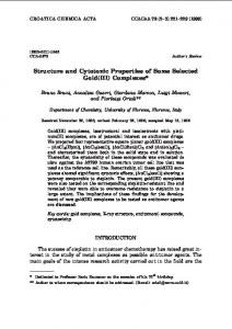
Figure 5: Mean error of robot pushing. Figure left shows the mean error calculated using Eq. (4) and all measurements. Figure right shows the incremental statistical evaluation as realized by oacpush .updateM. Four different objects were used in the experiment. the network can be refined incrementally. Statistical evaluation is also done incrementally as experiments are performed. Note however, that since the prediction function oacpush .updateTB changes during learning, the statistical evaluation oacpush .updateM only converges to the true accuracy of the behavior once oacpush .T B becomes stable. The motion of the pushed object depends on the object shape. Shape of the object is expressed as a low resolution binary image, which is used as an input to a neural network. In this way the system is able to learn a transformation function that does not need to be acquired separately for each object. 4.3.3
Incremental learning by exploration
There are two modes of operation in which we consider oacpush : A. initial learning of the prediction function oacpush .T B and the associated control policy, where the pushing directions encoded by a are randomly selected, and B. pushing the object towards a given target trg, where the current pusher movement a is determined based on the previously learned prediction function and the given target location. The prediction function oacpush .T B is essentially encoded by a neural network with the low resolution, binary image of an object as input values and the predicted movement of the pushed object as output. Note, that the 24
contact point on the object boundary and the angle of push are encoded in the object image and are therefore indirectly used as input values. Thus in mode B we calculate the optimal pusher movement a by first determining the desired Cartesian movement of o from its current location towards the target location and then inverting the neural network using nonlinear optimisation. The resulting behaviour is presented in Fig. 4. The learning process has been implemented using the following exploration behaviour: D = ∅; while true do repeat level = oacpush .level(); a = SelectRandomMotion; expr = level.execute(push, loc(o), bin(o), a); if level.eval(push, expr, ”the object has moved”) then D = D ∪ {expr}; oacpush .updateM(expr); end until enough data collected ; oacpush .updateT(D); end The inner repeat loop was implemented to allow for both batch and incremental learning. In this context generalisation means calculating parameters B of the transformation function oacpush .T B . Note that oacpush .updateM is always applied to data that was not used for learning.
4.4 4.4.1
Rule-Based Action Sequences: oacrule (o) Description
oacrule (o) is a symbolic description of cause-effects of the world in the highest level of abstraction. This OAC has been implmente on the humanoid robot ARMAR at UniKarl. In contrast to lower level OACs, like the grasping and pushing OACs, in this case the perceptions and actions are described with abstract references to lower level entities suitable to be used in the highest layer of the architecture as action rules for high level tasks completion. Actions in the oacrule (o) are commands that reference particular skills, like grasp(object) or push(object), but the execution of these commands are in charge of lower level mechanisms. Likewise, perceptions are described as boolean attributes. The oacrule (o) is in close relation to the planning OAC
25
of the next section as its instantiations have a STRIPS-like structure and can be used as planning operators for deliberation [2], [3]. In this section a simple example of a oacrule (o) is presented where the OAC is used to move objects on a plain surface in a controlled way. Given a scenario with objects and movement restrictions, the oacrule codes the necessary scenario configuration needed to move an object from its current position and orientation to a final position and orientation without colliding with other objects. oacrule is suitable for those scenarios with difficult accessibility and with many objects blocking each other, like the shelf of a fridge, a drawer or the shelf of a cupboard. oacrule is progressively refined from experience using a constructive learning approach to find the minimal sets of relevant attributes that afford movements of objects. These minimal sets of attributes are obtained from specialization of an initial set of attributes that codes the observed changes in the world after a first experience of an action. Specialization consists in adding necessary attributes to the precondition part of the rules to afford a given movement without collisions. The learning method applied for rule refinement is a constructive induction approach that performs a general to specific beam search of set of attributes with a probabilistic performance evaluation [3]. To illustrate the method, a simple scenario with glasses will be used to clarify the description of the OAC. For instance, figure 6 shows how a real world situation is internally represented by the robot using logic attributes and an example of a rule for moving a glass from its position (glass in cell 4 in the example) to another (cell 6). A detailed description of the example follows in the text below. 4.4.2
Definition
oacrule is defined by oacrule := ( rule; {in cell(oT , goal cell) == true, in angle(oT , goal angle) == true}; M) where oT accounts for the object to be moved (target object). Initial attribute space oacrule .A: The initial attribute space consists in a set of boolean attributes indicating the cell position and orientation angle 26
(discretized) of the target object ’oT ’, cells and angles of the other objects ’oj ’ in the scene, and indications about which cells are empty. Additionally to cells and angles, there is a couple of boolean attributes associated to each object which indicate whether the object is graspable or pushable. • in cell(o, icell), true if the object o is in cell number icell. • in angle(o, iangle), true if the object o has an orientation with an angle lying in the discretization segment iangle. • empty(icell), true if cell icell is empty.
Figure 6: Example of a scenario with glasses. A) Example of a state representation where the green glass is denoted as glass1 , red glass as glass2 , and blue glass as glass3 . B) One example of a rule for moving the green glass from cell 4 to cell 6 together with three possible hypothesis for rule specialization when surprises occur. Gray cells in the position representation indicates a “don’t care” if the cell is occupied by a glass or not.
27
• pushable(o), true if object o is pushable. • graspable(o), true if object o is graspable. As an example, the real world situation of figure 6(A) is internally rep-
Figure 7: Evolution of probabilities of success for the three hypothesis H1, H2 and H3, in the example of figure 6 for a sequence of seven experienced states. Black arrows indicate those situations where the rule in the example for moving green glass from cell 4 to cell 6 is applicable and tried. Arrows with a red cross reference to those situations where a blocking object prevent to obtain the desired outcome while not crossed arrows accounts for successful executions. Situations not marked with an arrow can not be used for the example rule updating as other rules are applied. 28
resented by the agent under a close world assumption as,
state = {empty(0), in cell(glass2 , 1), empty(2), empty(3), in cell(glass3 , 4), in cell(glass1 , 5), empty(6), empty(7), empty(8), empty(9), empty(10), empty(11), graspable(glass1 ), graspable(glass2 ), graspable(glass3 )}
where the green glass is considered as the target object and orientations are neglected as they are not relevant for the task. Prediction function oacrule .T : The prediction function returns a true for the target object in the goal cell and orientation angle,
{in cell(oT , goal cell) == true, in angle(oT , goal angle) == true}
In the glasses example of figure 6, the prediction of the application of the OAC for moving the green glass to 6 is,
goal = {in cell(glassT , 6)} ˆ The predicted attribute space is Predicted attribute space oacrule .A: given by all the possible goal cells and goal orientation angles. Evaluation: level.eval checks if the final cell position and orientation angle of the target object oT after the action execution is the same as the goal cell and goal angle. Whenever this is the case the expr is considered as successful. Execution level.execute: The highest chance of success has associated a rule with an action that is selected for its execution, + Pgoal =
max
∀rule∈activerules
+ Prule ( goal|A, a);
(5)
This probability is extracted from the active rule with highest chance of returning the goal after its associated action execution. Active rules are those which preconditions are included in the observed state A. 29
When the process of execution is triggered the action of that rule is passed to the lower level mechanisms as a command. The action consists in movements of translation and rotation performed over objects. The movement could be done by either grasping the object and then placing it in the final position and orientation (skill = grasp), or by pushing it until the final position and orientation are reached (skill = push), a = move(˜ o, f inal cell, f inal angle, skill);
(6)
Note that in the example of figures 6 and 7 it is assumed that no changes are obtained after an action execution if there is an object blocking the movement. Generalization oacrule .updateActionParams: To a rule the probability of obtaining the goal position and orientation after applying its related action a becomes associated. The associated proba+ (goal|A, a) bility of success and failure in the predictions are denoted as Prule − and Prule (goal|A, a) respectively. As we will see these probabilities will be used for the oacrule refinement in the learning function. In order to calculate the probabilities of success (or failure) for rule selection and execution two numbers are stored for each rule, • n+ rule , counter for successful predictions of the goal when the rule is activated. • n− rule , counter for failed predictions of the goal when the rule is activated. The probabilities related to the success or failure in the prediction, − + (goal|A, a), are calculated as, (goal|A, a) and Prule Prule 1 + Prule (goal|A, a) = 2 1 − Prule (goal|A, a) = 2
1+
1+
n+ goal|A,a ntotal goal|A,a n− goal|A,a ntotal goal|A,a
−
−
n− goal|A,a
! (7)
ntotal goal|A,a n+ goal|A,a ntotal goal|A,a
! (8)
where ntotal rule is the total number of possible states where the rule could be activated. + With these formulas a high Prule ( goal|A, a) is a confident indicator of a good chance of obtaining the prediction because the probabilities are based 30
on densities of samples and assign to unexplored states the same chance to result in a successful or failed prediction. Statistics fed only a few times with a successful prediction would result in a probability of a positive a little higher than 0,5. Others evaluation criteria based on relative frequencies, like the entropy or the m-estimate, would indicate a high chance of obtaining a success even with a few examples. Figure 7 exemplifies how the probabilities of success evolves for the three hypothesis about preconditions stated in figure 6. Generalization is performed using a constructive induction approach to find rules with the minimal sets of initial attributes to obtain the goal state after executing action a (see [3] for details). The rule representation is progressively refined from experience using a general to specific beam search and memorized experiments expr [3]. Whenever a rule has high uncertainty in its prediction (prob. close to 0,5) and large confidence (high density of samples), it is refined by generating new specializations of the rule using the information gain criterion. The density of samples is calculated as, ρrule =
4.5 4.5.1
+ n− rule + nrule ≤1 ntotal rule
(9)
Planning OAC Description
The following is a simple example of a grasping OAC for use by an AI planner. OACs like the following form the basis of the high level planning in the PACO-PLUS system. It is the predictive nature of these OACs that allow us to anticipate the effects of actions and correctly choose OACs that will achieve our objectives. This example OAC is based loosely on the AI planning level “graspA-fromTable” action that is used in UEdin integration with SDU. (See PACO-PLUS deliverable 4.3.1 for details). Following the definitions in Section 3.1 we will provide an OAC that defines grasping over the global attribute space, S given in Table 1 4.5.2
Definition
An OAC to capture grasping for use in planning is defined by
31
Properties clear(?x)
A predicate indicating that no object is stacked in ?x.
gripperEmpty
A predicate describing whether the robot’s gripper is empty or not. A predicate indicating that the robot is holding object ?x in its gripper. A predicate indicating that object ?x is in a stack with object ?y at its base. A predicate indicating that object ?x is stacked in object ?y. A predicate indicating that object ?x is on the shelf. A predicate indicating that object ?x is on the table. A predicate indicating that object ?x is open. A function indicating that the radius of object ?x is ?y. Predicates indicating that object ?x is reachable by the gripper using a particular grasp. A function indicating that there are ?x empty shelf spaces.
inGripper(?x) inStack(?x,?y) isIn(?x,?y) onShelf(?x) onTable(?x) open(?x) radius(?x) = ?y reachable(?x) shelfSpace = ?x
Table 1: Attribute Space for planning level OACs
oac = (gPlan; T; M) To define an OAC we provide an identifier, a prediction function, T defined on this level’s S, and a statistical measure of the OAC’s prediction success, M . Since the identifier for the OAC is only used to allow communication about OACs at different levels we will have little to say about it. In this case without loss of generality we will assume it is something like, gPlan. Given a level with the state space, S, as defined in Table 1, we can define the prediction function, T , for our OAC as the first order logical rule given in Table 2. In this case, both the initial conditions and the predictions are Name grasp-fromTable(?x)
Initial Conditions reachable(?x) clear(?x) gripperEmpty onTable(?x)
Prediction inGripper(?x) not(gripperEmpty) not(onTable(?x))
Table 2: OAC prediction function, T , for a planning level grasping action. 32
assumed to be conjunctive (that is, all of the initial conditions of the rule must be true in the world for the prediction function to be defined, and all of the terms of the prediction are expected to be true in any state that results from the execution of the OAC). Therefore, this function states that if an object is on the table, the object is clear, the object is reachable, and the gripper is empty, then if this OAC is executed we predict the object will be in the gripper and not on the table. In any other case, the resulting state is undefined. We must also provide a statistical measure of the success of T , M . Taking the simplest possible approach, we define M as the long term probability of T correctly predicting the resulting state given the execution of the OAC from an initial state for which the OAC is defined. Note that in classical AI planning systems like STRIPS [18], M for this OAC would therefore be fixed at one. Such classical planners assumed a deterministic and totally observable world removing any uncertainty in their prediction functions. More recent work in AI planning of course has moved beyond these far too limiting assumptions [16]. There are now a number of AI planning algorithms that are able to make use of probabilistic statements about the long term success of this kind of prediction to build probabilistic plans for actions. Thus in PACO-PLUS we define M as the long term accuracy of the OAC’s prediction function. UEdin’s work on learning action representations [13] produces OAC representations that are isomorphic to that shown here, and we refer the interested reader to PACO-PLUS deliverable 5.1.2 for an account of how this kind of OAC (both the symbolic prediction function and the associated M ) can be learned. PACO-PLUS deliverable 4.3.5 outlines an interaction architecture for executing these kinds of OACs. In general, we anticipate the execution function for this kind of OAC would involve the invocation of a more specific OACs (see Sections 4.2 and 4.3) designed to implement specific grasping behavior on the robot hardware. This highlights a number of open issues in this set of definitions including: 1. how the mapping to this lower level OAC is encoded and performed, 2. how the arguments to the called OAC are determined, stored, and updated, 3. and more generally how objects are represented in the system as a whole. The implementation of the PACO-PLUS project has made a number of 33
pragmatic decisions to answer these questions (again outlined in deliverable 4.3.5) that currently fall outside the scope of these OAC definitions. 4.5.3
Using this OAC in practice
OACs like this one are currently used in PACO-PLUS within the PKS system [16] to build plans for stacking and unstacking of containers in a kitchen like environment. We refer the interested reader to PACO-PLUS deliverable 4.3.5 for details of the encoding of actions for this domain and their use by a planner.
5
Outstanding Issues
In summary, PACO-PLUS project views object-action complexes as a dynamic (learnable, refinable) and grounded representation that binds objects, actions and attributes associated with an agent in a strong, causal way. They can carry low-level (sensorimotor) as well as high-level (symbolic) information and can thereby be used to join the perception-action space of an agent with its planning-reasoning space. In addtion, they enforce the storage of relevant information for further bootstrapping in episodic memory. These properties open an avenue for addressing several important research challenges in the cognitive sciences in the future. Addressing these questions, we might find that extensions or modifications of the original OAC definition might be required. At least the following challenges arise for the last year of the project and beyond: C1 Interactions between OACs – (Linking levels) The relationship between OACs at different levels of abstraction for execution and learning needs to be investigated further. Rigorous formal algorithms for this interaction need to be designed. – (Continuity) How can we realize seamless and continuous switching and sequencing of OACs at the same or at different levels of abstraction? – (Stability) How can stability be achieved in a system that makes use of dynamic OACs as sub–modules with temporally varying success likelihoods?
34
C2 Bootstrapping processes making use of the episodic memory: The stored experiments provide the data for further learning processes across OACs generalizing actions across objects (such as learning more general part–action associations), emergence of perceptual categories etc. For example, based on such a memory process an agent could try to address the following three issues: – (Categorization) How to realize that OAC sequences leading to similar state space transitions define similar objects (e.g., pouring water in object Ai leads to positive weight change in object Ai suggests all objects Ai to be containers)? – (Generalization) How detect and utilize re-occurrences of perceptual attribute–action combinations as for example in the learning of part–action associations? – How to address the learning of cause-effect couples and the learning of pre-conditions, where both ultimately would lead to new planning rules ([2]). – (Efficiency) How to efficiently distribute resources that are required for learning (on-line versus batch learning requiring storage in episodic memory). C3 Development of OACs: Critically within a system based on OACs, interactions with the environment can lead to the creation of new OACs. Such new OACs can be at varying levels of abstraction. We can imagine learning new complex very low level skills (like how to effectively move my foot so as to kick a soccer ball along a desired trajectory) to a high level action (like learning that once I have passed the soccer ball to my team mate I no longer have it). Identifying when to create a new OAC as opposed to modifying an existing OAC is a critical research area for understanding the power of OACs and how and when they will allow us to make use of existing work to ground our systems in real world experience. C4 Extension of the attribute space: OAC based interaction with the environment can also result in learning new attributes. As such it will also be critical to develop a formal model of how and when the attribute space that OACs are defined on are extended and expanded. We must provide an answer to the critical questions of when new attributes should be added to the space, as opposed to when existing
35
attributes should be refined. We note that this may even require rethinking the kinds of learning algorithms that we use to learn OACs since many existing algorithms for learning require a fixed attribute space to work in or are not amenable to the incremental learning that is inherent in an OAC based interaction with the world. This list is certainly incomplete and it is to be expected that it will have to be extended in the course of future work. We believe, however, that the OAC concept provides a solid starting point for discussing, defining and addressing future challenges and that OACs will act as a glue for future research in artificial cognition.
A
Additional Notes on the Statistical Evaluation of an OAC Using an Arbitrary Metric
Computing a statistical evaluation of the empirical success of an OAC can involve (in addition to the binary success/failure statement) a quantitative comparison of the expected and actual outcomes. This requires the measureˆ We define the change ment of the initial (A) and resulting attributes (A). j j in attribute A (where A covers both world and internal attributes) after executing an OAC as: ∆Aj = dj (Aˆj , T (Ajt ))
(10)
where dj is a metric that makes the difference in every attribute Aj measurable (i.e., it allows for a meaningful subtraction operation in this equation). T (Aj ) is the restriction of T to the j-th attribute. Clearly dj will be different for different attribute types like continuously encoded quantities, discrete non-countable entities (hollow versus solid), rank attributes, relational attributes. The application of dj , however, assures that ∆Aj becomes independent of the attribute as such (invariance property of the change). An example for ∆Aj could be the changed filling level of a cup after a drinking action.8 As a default setting for the components of M (which however can be replaced by other statistical definitions with similar meaning), we can define ˜ hi = M j
N X
wi ∆Aji
(11)
i=1 8
Note that eval can now be defined by thresholding operations over the ∆Aj , for P j 1 example by setting eval = 1 if N i ∆A > Θ, else = 0.
36
the average change of a single attribute Aˆj after N executions of the iOAC. N is the number of executions of the OAC. In addition we have the weighted standard deviation: ˜ σ := PN wi (M ˜ hi − ∆Aj )2 . M j i=1 j where wi decodes a suitable window function (with wi > 0 for all i and P wi = 1) weighting recent experiences more than past ones. Note, so far we have defined all these entities for each individual attribute j. If necessary, this definition can be extended to the averaging over all attributes ˜ hi = 1 PK µj M ˜ hi , and likewise for the variance, where µj weighs using M k=1 j K different attributes differently. In the examples we will, thus, drop index j assuming that averaging across attributes has taken place (if necessary).
References [1] D. Aarno, J. Sommerfeld, D. Kragic, N. Pugeault, S. Kalkan, F. W¨ org¨ otter, D. Kraft, and N. Kr¨ uger. Early reactive grasping with second order 3d feature relations. In The IEEE International Conference on Advanced Robotics, Jeju Island, Korea, 2007. [2] A. Agostini, E. Celaya, C. Torras, and F. W¨org¨otter. Action rule induction from cause-effect pairs learned through robot-teacher interaction. In Proc. International Conference on Cognitive Systems, pages 213–218, Karlsruhe, Germany, 2008. [3] A. Agostini, F. W¨ org¨ otter, E. Celaya, and C. Torras. On-line learning of macro planning operators using probabilistic estimations of causeeffects. Technical Report IRI-TR 05/2008, Institut de Rob`otica i Inform` atica Industrial, UPC-CSIC, Barcelona, Spain, 2008. [4] R. Detry, M. Popovic, Y. P. Touati, E. Baseski, N. Kr¨ uger, and J. Piater. Autonomuous learning of object-specific grasp affordance densities. In ICRA Workshop Approaches to Sensorimotor Learning on Humanoid Robots, pages 36–37, Kobe, Japan, 2009. [5] R. Detry, N. Pugeault, and J. Piater. A probabilistic framework for 3D visual object representation. IEEE Transactions on Pattern Analysis and Machine Intelligence, accepted. [6] N. Fikes. STRIPS: a new approach to the application of theorem proving to problem solving. Artificial Intelligence, 2(3-4):189–208, 1971. 37
[7] C. Geib, K. Mour˜ ao, R. Petrick, N. Pugeault, M. Steedman, N. Kr¨ uger, and F. W¨ org¨ otter. Object action complexes as an interface for planning and robot control. In Workshop ’Toward Cognitive Humanoid Robots’ at IEEE-RAS International Conference on Humanoid Robots, Genoa, Italy, 2006. [8] J. J. Gibson. The Perception of the Visual World. Houghton Mifflin, Boston, 1950. [9] R. Kowalski and M. Sergot. A logic-based calculus of events. New Generation Computing, 4:67–95, 1986. [10] D. Kraft, E. Ba¸seski, M. Popovi´c, A. M. Batog, A. Kjær-Nielsen, N. Kr¨ uger, R. Petrick, C. Geib, N. Pugeault, M. Steedman, T. Asfour, R. Dillmann, S. Kalkan, F. W¨org¨otter, B. Hommel, R. Detry, and J. Piater. Exploration and planning in a three level cognitive architecture. In Proc. International Conference on Cognitive Systems, pages 71–78, Karlsruhe, Germany, 2008. [11] D. Kraft, N. Pugeault, E. Ba¸seski, M. Popovi´c, D. Kragic, S. Kalkan, F. W¨ org¨ otter, and N. Kr¨ uger. Birth of the Object: Detection of Objectness and Extraction of Object Shape through Object Action Complexes. International Journal of Humanoid Robotics, 5(2):247–265, 2008. [12] N. Kr¨ uger, M. Lappe, and F. W¨org¨otter. Biologically Motivated Multimodal Processing of Visual Primitives. The Interdisciplinary Journal of Artificial Intelligence and the Simulation of Behaviour, 1(5):417–427, 2004. [13] K. Mour˜ ao, R. P. A. Petrick, and M. Steedman. Using kernel perceptrons to learn action effects for planning. In Proc. International Conference on Cognitive Systems, pages 45–50, Karlsruhe, Germany, 2008. [14] D. Omrˇcen, A. Ude, and A. Kos. Learning primitive actions through object exploration. In Proc IEEE-RAS International Conference on Humanoid Robots, Daejeon, Korea, pages 306–311, 2008. [15] R. Petrick, D. Kraft, K. Mour˜ao, C. Geib, N. Pugeault, N. Kr¨ uger, and M. Steedman. Representation and integration: Combining robot control, high-level planning, and action learning. In Proc. 6th International Cognitive Robotics Workshop, Patras, Greece, 2008.
38
[16] R. P. A. Petrick and F. Bacchus. A knowledge-based approach to planning with incomplete information and sensing. In Proc. of AIPS-02, pages 212–221, 2002. [17] M. Popovic, D. Kraft, L. Bodenhagen, E. Baseski, N. Pugeault, D. Kragic, and N. Kr¨ uger. A strategy for grasping unknown objects based on co-planarity and colour information. Robotics and Autonomous Systems, (submitted). [18] S. Russell and P. Norvig. Artificial Intelligence: a Modern Approach. Prentice Hall, Upper Saddle River, NJ, 2nd edition, 2003. ¨ [19] E. Sahin, M. Cakmak, M. R. Dogar, E. Ugur, and G. Ucoluk. To afford or not to afford: A new formalization of affordances toward affordancebased robot control. Adaptive Behavior, 15(4):447–472, 2007. [20] M. Steedman. Plans, affordances, and combinatory grammar. Linguistics and Philosophy, 25(5-6):723–53, 2002. [21] F. W¨ org¨ otter, A. Agostini, N. Kr¨ uger, N. Shylo, and B. Porr. Cognitive agents — A procedural perspective relying on the predictability of Object-Action-Complexes (OACs). Robotics and Autonomous Systems, 57(4):420–432, 2009.
39