Hindawi Publishing Corporation Advances in Mechanical Engineering Volume 2013, Article ID 357920, 11 pages http://dx.doi.org/10.1155/2013/357920
Research Article A Fourier Series-Neural Network Based Real-Time Compensation Approach for Geometric and Thermal Errors of CNC Milling Machines Wei Wang, Yi Zhang, Kaiguo Fan, and Jianguo Yang School of Mechanical Engineering, Shanghai Jiao Tong University, Shanghai 200240, China Correspondence should be addressed to Wei Wang;
[email protected] Received 3 April 2013; Accepted 30 July 2013 Academic Editor: C. S. Shin Copyright © 2013 Wei Wang et al. This is an open access article distributed under the Creative Commons Attribution License, which permits unrestricted use, distribution, and reproduction in any medium, provided the original work is properly cited. In order to improve the accuracy and efficiency of the real-time error compensation, a Fourier Series-Neural Network (FS-NN) based compensation methodology is developed to reduce the thermally induced geometric errors of CNC milling machines under varying conditions. Firstly, an error model is presented based on the principle of Fourier series with fast calculation and higher precision, which is regarded as the error base of original geometric errors. Secondly, the relationships between the slopes related to different error curves and the temperatures of key thermal points are figured out by using neural networks when concerning thermal effects. Then, a combined error model is established which is suitable for reducing axis positioning errors at any thermal status. Finally, a real-time dynamic error compensation system is developed featuring automatic error modeling and multiaxis synchronous compensation. The experimental results prove that the proposed methodology has satisfactory modeling accuracy and robustness to frequently changing working conditions.
1. Introduction It has been verified that thermally induced error is one of the most significant sources of machine tool inaccuracy, which accounts for 40%–70% of total errors [1, 2]. In recent years, researchers have considered many ways of error reduction in machine tools, especially for the minimization of thermal influence including thermally optimized machine structure design, separation of heat sources, and improved cooling system [3, 4]. However, due to the limited accuracy improvement of these methods, the associated manufacturing costs can be very high. Therefore, the cost-effective real-time error compensation technique is of great importance to the accuracy improvement of CNC machine tools [5]. In some modern high-precision machine tools, built-in error compensation function is provided by the CNC system in parameter setup. The predicted error data is input to the error compensation setup function, which is called leadscrew compensation. In the actual machining process, these
preloaded errors are added to the mathematical calculation step in the CNC system. Methods for implementing leadscrew compensation can be found in [6, 7]. It is accomplished by creating a table of the positioning errors corresponding to a serial of points at fixed intervals. The compensation values for any points between the fixed intervals are simply calculated by linear interpolation and then input to the CNC control system. This kind of compensation is generally quick to measure and to apply, and it really does work well for cases where the positioning errors are consistent at the measuring moment and the compensating moment. However, it is limited in a certain condition especially when the environmental temperature stands still or varies a little. If the machine is not in a constant-temperature workshop or when the thermal error fluctuates due to the variation of machine tool temperature field, error table is useless unless a new one is made; otherwise the compensation result will not be satisfying. Therefore, using the above-mentioned method, the thermal error cannot be real-time compensated in the actual machining process. Yet considering all the error factors
2 in a machine tool, the thermally induced error contributes a large proportion and directly affects the machining precision of work piece to a considerable degree [8]. External software compensation is an effective way to essentially eliminate the machining error at a low cost, and it is attracting increasing attention in the manufacturing industry [9]. Effective software error compensation depending on mathematic models is commonly used. The models can accurately map the empirical relationship between discrete temperature data of several points and the thermal deformation of machine tools [10, 11]. A number of research works have been done in the past. Chen made a multiple regression analysis and proposed the artificial neural network model for the real-time forecast of thermal errors with numerous temperature measurements [12]. Lee et al. presented a thermal modeling method based on independent component analysis to compensate for the thermal errors of a commercial machining center [13]. Wang et al. established an error model of thermally induced geometric errors for a milling center based on Newton interpolation method [14]. Li et al. and Yan and Yang optimized the thermal sensor’s placement on machine tools based on the gray correlation model and decreased the number of temperature variables [15, 16]. Wang and Tseng adopted the k-means theory to classify the obtained thermal data, which was especially useful in a working environment in which engineers were facing the urgent requirement for a fast, easily programmed modeling method [17]. Though the above-mentioned approaches show a satisfactory predictive accuracy in many occasions, most of them are empirical and highly dependent on the data collected from specific types of machine tools. It is hard to build a mathematical model with higher accuracy and robustness using these methods, which prevents the widespread application of thermal error compensation. Besides, some mathematical calculations are quite complicated and not suitable in a real-time error compensation system. So there is still room for the improvement of mathematical model with wider range of application, higher accuracy, and robustness. This paper mainly focuses on the thermally induced geometric error compensation, particularly in machine feed axes. The Fourier series algorithm is employed to approximate the error base of original geometric errors of a vertical milling center. This algorithm is ideal for fitting the periodic fluctuations of error data with fast calculation and higher precision, thereby benefiting for the real-time error compensation. For the situation of feed axis error modeling, the error is related not only to the key thermal points but also to the coordinates of translational axes. Therefore, the neural network is used to establish the relationship of machine temperature rise and slope of varied error curves which contributes to the mixed error model. Real-time error compensation is achieved by means of a proposed error compensation system featuring automatic error modeling and multiaxis synchronous compensation. The effectiveness of the derived synthesis error model based on the proposed approach is verified through the experiments.
Advances in Mechanical Engineering
Figure 1: Positioning error measurement.
2. Methodology 2.1. Experimental Setup. The CNC machine used in this research is a high-precision VM850 milling center. The machine CNC is the FANUC 0i CNC system from FANUC Corporation and the laser interferometer is a XL-80 Laser Measurement System from Renishaw Inc. The setup of the experiments consists of five major steps: (1) configuring the laser interferometer system and the milling center control to measure the positioning accuracy of the axis; arranging the thermistors on the milling center; (2) running the milling center and laser system to collect the measurement data; rising up the machine to some specific moments and recording the temperature values; (3) error modeling with the measured data; (4) programming the real-time calculations in error compensation system for integrating into the CNC controller; (5) Repeating the measurement test to determine the real performance of the system. The measurement of machine axis positioning error is shown in Figure 1. To reduce the random error in measuring process, every axis was repeatedly measured triple times in both forward direction and backward direction. The medium values were kept as the final measuring result. The travel range, of 𝑋-, 𝑌- and 𝑍-axes were set to 800 mm, 400 mm, and 400 mm, respectively, and the measurement started from the origin of machine coordinates. The machine ran in 𝑌- or 𝑍-axis direction and paused at every 25 mm distance (paused at every 50 mm for 𝑋-axis) where the error data was recorded as the measuring point. In order to evaluate the machine tool positioning error synthetically, the temperature variations and positioning errors were measured in different machine tool temperatures. First, the machine tool positioning error in normal temperature was measured when the machine started running; then the machine is warmed up by moving the slides at a feed rate of 3 m/min along the 𝑋-, 𝑌-, and 𝑍- directions. Afterwards, the machine temperature was rising while the error data at different times were measured, and this process
Advances in Mechanical Engineering
T1
26 T2
T5
Temperature (∘C)
T4
3
23 20 17
0
20
T3, T6 T0 T1 T2 T3
Figure 2: Thermal sensor locations.
40
60 Time (min)
80
100
120
T4 T5 T6 T7
Figure 3: Temperature variations.
was repeated to make the machine temperature rise to the thermal equilibrium state. At this moment, the measuring process was done. The temperature rising times at 10 min, 20 min, 30 min, 45 min, 70 min, and 120 min were chosen for further consideration. The machine temperature curves varied sharply in the initial moment, so the temperature rising time was shorter. While measuring the positioning error, the machine temperature was also needed to be obtained. Therefore, each positioning error data corresponded to a specific series of machine temperature data. To measure the temperature, eight thermistors were attached to the key thermal points which were directly related to the thermal deformation of feed axis: T0 was used to measure the room temperature; T1, T2, and T3 were set on the screw nut of 𝑋-, 𝑌-, and 𝑍-axes, respectively; T4, T5, and T6 were set on the guide way of 𝑋-, 𝑌-, and 𝑍axes, respectively; T7 was used to measure the temperature of machine body. The arrangements of thermistors from T1 to T6 are shown in Figure 2. Throughout the whole temperature rising process, an automatic temperature acquisition software developed with LabVIEW was used to real-time detect the temperature variations. When the measuring time started, the temperature data of each observing points was recorded. The results are shown in Figure 3. In order to better understand the thermal influence on machine mechanical component, thermal expansion is considered according to Figure 3. The 40 Cr is one of the most commonly used materials for lead screw. Taking 40 Cr for example, the linear coefficient of thermal expansion (CTE) is 12.5 ppm/∘ C at room temperature 20∘ C. According to Figure 3, a 40 Cr lead screw with original length (L) 0.4 m will expand, Δ𝐿 = 𝛼 ⋅ 𝐿 ⋅ Δ𝑇 = 12.5 ⋅ 0.4 ⋅ 8 = 40 ppm, as the temperature increases by 8∘ C. This expansion is a problem that should be paid much attention.
error curves, it is obviously that every positioning error measured in different temperatures varies sharply. This is the reason why lead-screw error compensation method has no effects on changing temperatures. The table of the positioning errors made by lead-screw method is carried out according to only one positioning error curve rather than an overall analysis on the entire error curves. Hence, with different temperature data, the compensation should be implemented based on different positioning error curves. Furthermore, automatic error compensation is also needed through some novel methods neglecting the complicated making process of error table. According to Figure 4, as the machine temperature is rising, each error curve varies a little in shape, but the curve slope differs. Therefore, this error modeling process can be separated into the following two parts: the geometric component and the thermal component. The geometric component of linear positioning error is only related to the machine coordinate position while the thermal component of linear positioning error is also related to the machine temperature. In this study, 17 measured points can be obtained in each error curve through each axis travel. To make it as a general rule, the original positioning error sequence with n intervals in normal temperature can be expressed as
2.2. Error Modeling. The seven positioning error measurements from 0 to 120 min temperature rise are chosen and the error curves are shown in Figure 4. According to the
where 𝑖 = 1, 2, . . . , 𝑁. Linear fitting is made separately on the seven error curves at different temperature rising time in Figure 4. The fitting
𝑥1(0) = (𝑥1(0) (1) , 𝑥1(0) (2) , . . . , 𝑥1(0) (𝑛)) .
(1)
And all the error sequences from normal temperature to the latest temperature rise are expressed as 𝑥𝑖(0) = (𝑥𝑖(0) (1) , 𝑥𝑖(0) (2) , . . . , 𝑥𝑖(0) (𝑛)) ,
(2)
4
Advances in Mechanical Engineering Table 1: The coincidence relations.
Error (𝜇m)
20
Position/mm X|YZ
10 0 −10 −20 0
100
200
300
400
500
600
700
800
300
350
400
X-axis travel (mm)
Error (𝜇m)
20 10 0 −10 −20 0
50
100
150
200
250
Y-axis travel (mm)
−1.0 0.2 −0.7 −3.4 −4.4 −4.7 −2.5 −2.6 −1.5 −1.9 −1.5 −0.8 −2.9 −1.9 0.1 −2.2 −3.0
Mean value of error points/𝜇m Z Y 5.6 3.1 10.3 −2.4 8.5 −1.5 11.7 0.1 13.6 −0.2 12.9 −0.7 14.9 −0.6 13.6 −0.4 13.2 −2 13.3 1.4 11.6 1.8 11.5 3.2 11.1 2.6 11.4 −0.3 9.8 −2.5 8.9 −1.4 8.7 −0.8
the linear fitting lines across the ordinate at the origin point. This step can be calculated as follows:
20 Error (𝜇m)
0|0 50|25 100|50 150|75 200|100 250|125 300|150 350|175 400|200 450|225 500|250 550|275 600|300 650|325 700|350 750|375 800|400
X
10
𝑥𝑖(1) = 𝑥𝑖(0) − 𝑘𝑖𝑇 𝑥𝑖(0) (𝑛) + 𝑏𝑖∧ ,
0 −10 −20 0
50
100
150
200
250
300
350
400
Z-axis travel (mm)
45 min 70 min 120 min
0 min 10 min 20 min 30 min
(4)
where 𝑏𝑖∧ is the mean value of 𝑏𝑖 . In the next step, the average value of the rotated seven error curves is calculated and the mean value of error points for 𝑋-, 𝑌-, and 𝑍- axes is shown in Table 1. A standard error curve is obtained including a serial of all the measurement points: 1 𝑛 1 𝑛 { ∑𝑥𝑖(1) } = {∑ [𝑥𝑖(0) − 𝑘𝑖 𝑇 𝑥𝑖(0) (1) + 𝑏𝑖∧ ] , 𝑛 𝑖=1 𝑛 𝑖=1 𝑛
∑ [𝑥𝑖(0) − 𝑘𝑖 𝑇 𝑥𝑖(0) (2) + 𝑏𝑖∧ ] , . . . ,
Figure 4: Positioning errors at varied temperatures.
(5)
𝑖=1 𝑛
lines are illustrated in the following equation, thereby all the slopes of each error curve are obtained for the next step, 𝑇
(𝛿0 , 𝛿1 , . . . , 𝛿𝑛 ) = 𝑘𝑖 𝑇 𝑥 + 𝑏𝑖 , 𝑘𝑖 = 𝑘0 , 𝑘1 , . . . , 𝑘𝑛 ,
(3)
where 𝑖 = 1, 2, . . . , 𝑛, 𝛿0 , . . . , 𝛿𝑛 refers to each fitting line and 𝑘𝑖 is the slope of each fitting line. In order to obtain the reference error curve as the standard modeling curve, first, turn all the error curves into horizontal direction to make their slopes zero. These error curves are revolved around a fixed mean value point where
∑ [𝑥𝑖(0) − 𝑘𝑖 𝑇 𝑥𝑖(0) (𝑛) + 𝑏𝑖∧ ]} . 𝑖=1
In order to find the inherent regularity from these discrete data points, we need to take advantage of these data points to obtain an approximation by generating a new function. These discrete points are distributed around the central line and continuously fluctuate, which suggests that they can be described by Fourier series in the segmented range. In this research, a Fourier series model is adopted to optimize the error fitting. It is represented in either the trigonometric form or the exponential form. The following functions are based on the trigonometric Fourier series form. Using Fourier series fitting, the reference curve is represented as the sum of a series of sinusoidal and cosinoidal waves.
Advances in Mechanical Engineering
5
Assume that 𝑓(𝑥) is a periodic function of period 2𝜋 and is integrable over a period: ∞
𝑓 (𝑥) ≃ 𝐴 0 + ∑ [𝐴 𝑛 cos (𝑛𝑥) + 𝐵𝑛 sin (𝑛𝑥)] .
(6)
𝑛=1
This is the expression of Fourier series and the coefficients are determined in the following part. Integrating on both sides of (6) from −𝜋 to 𝜋: 𝜋
𝜋
∞
𝜋
−𝜋
−𝜋
𝑛=1
−𝜋
∫ 𝑓 (𝑥) 𝑑𝑥 = ∫ 𝐴 0 𝑑𝑥 + ∑ 𝐴 𝑛 ∫ cos (𝑛𝑥) 𝑑𝑥 ∞
𝜋
𝑛=1
−𝜋
(7)
The last two integrations of trigonometric terms are equal to zero. Hence 1 𝜋 ∫ 𝑓 (𝑥) 𝑑𝑥. 2𝜋 −𝜋
̂ . [𝐽𝑇 𝑊𝐽 + 𝜆𝐼] ℎ𝑙𝑚 = 𝐽𝑇 𝑊 (𝑦 − 𝑦)
(8)
̂ , [𝐽𝑇 𝑊𝐽 + 𝜆 diag (𝐽𝑇 𝑊𝐽)] ℎ𝑙𝑚 = 𝐽𝑇 𝑊 (𝑦 − 𝑦)
Δ 𝑥 = 𝑎0 + 𝑎1 ⋅ cos (𝑥𝑤) + 𝑏1 ⋅ sin (𝑥𝑤) + 𝑎2 ⋅ cos (2𝑥𝑤) + 𝑏2 ⋅ sin (2𝑥𝑤) + 𝑎3 ⋅ cos (3𝑥𝑤) + 𝑏3 ⋅ sin (3𝑥𝑤)
𝜋
𝜋
+ 𝑎4 ⋅ cos (4𝑥𝑤) + 𝑏4 ⋅ sin (4𝑥𝑤)
−𝜋
−𝜋
∫ cos (𝑚𝑥) 𝑓 (𝑥) 𝑑𝑥 = ∫ 𝐴 0 cos (𝑚𝑥) 𝑑𝑥
= −2.117 + 0.0958 cos (0.006981𝑥)
𝜋
+ ∑ ∫ 𝐴 𝑛 cos (𝑛𝑥) cos (𝑚𝑥) 𝑑𝑥 𝑛=1 −𝜋 ∞
− 0.709 sin (0.006981𝑥) + 0.7477 cos (0.013962𝑥) + 0.4801 sin (0.013962𝑥) + 0.01371 cos (0.020943𝑥)
𝜋
+ ∑ ∫ 𝐵𝑛 sin (𝑛𝑥) cos (𝑚𝑥) 𝑑𝑥. 𝑛=1 −𝜋
(9) The only nonzero term on the right is when 𝑚 = 𝑛 in the first summation: 𝐴𝑛 =
(15)
is used in the Levenberg-Marquardt algorithm implemented in MATLAB [18]. According to the above algorithm, fourth Fourier fitting is used here which is suitable for the accuracy demand:
Multiply both sides of (6) by cos(𝑚𝑥) and integrate
∞
(14)
Marquardt’s suggested update relationship,
+ ∑ 𝐵𝑛 ∫ sin (𝑛𝑥) 𝑑𝑥.
𝐴0 =
To solve the nonlinear least squares problem, the Levenberg-Marquardt method is applied in the algorithm. The Levenberg-Marquardt curve-fitting method is actually a combination of two minimization methods: the gradient descent method and the Gauss-Newton method. The Levenberg-Marquardt algorithm adaptively varies the parameter updates between the gradient descent and GaussNewton update:
𝜋
1 ∫ 𝑓 (𝑥) cos (𝑛𝑥) 𝑑𝑥. 𝜋 −𝜋
(10)
+ 1.081 sin (0.020943𝑥) − 0.007711 cos (0.027924𝑥) + 0.8147 sin (0.027924𝑥) . (16) Using the same modeling method, the standard error approximations of both 𝑌-axis and 𝑍-axis can be calculated as Δ 𝑦 = [−175.4 + 279.9 cos (−0.0004079𝑥)
Multiply both sides of (6) by sin(𝑚𝑥) and integrate 𝜋
𝜋
− 20.16 sin (−0.0004079𝑥) − 139.1 cos (−0.0008158𝑥)
−𝜋
−𝜋
+ 20.13 sin (−0.0008158𝑥) + 39.29 cos (−0.0012237𝑥)
∫ sin (𝑚𝑥) 𝑓 (𝑥) 𝑑𝑥 = ∫ 𝐴 0 sin (𝑚𝑥) 𝑑𝑥 ∞
𝜋
+ ∑ ∫ 𝐴 𝑛 cos (𝑛𝑥) sin (𝑚𝑥) 𝑑𝑥 𝑛=1 −𝜋 ∞
𝜋
+ ∑ ∫ 𝐵𝑛 sin (𝑛𝑥) sin (𝑚𝑥) 𝑑𝑥. 𝑛=1 −𝜋
(11) The only nonzero term on the right is when 𝑚 = 𝑛 in the second summation: 1 𝜋 𝐵𝑛 = ∫ 𝑓 (𝑥) sin (𝑛𝑥) 𝑑𝑥. 𝜋 −𝜋
(12)
The least-squares fit of a sinusoidal function is to determine coefficient values that minimize 𝑁
2
𝑆 = ∑{𝑦𝑖 − [𝐴 0 + 𝐴 1 cos (𝜔0 𝑡𝑖 ) + 𝐵1 sin (𝜔0 𝑡𝑖 )]} . 𝑖=1
(13)
− 8.606 sin (−0.0012237𝑥) − 4.835 cos (−0.0016316𝑥) +1.43 sin (−0.0016316𝑥)] × 1010 , Δ 𝑧 = [−569.6 + 907 cos (−0.0004563𝑥) − 92.94 sin (−0.0004563𝑥) − 446.9 cos (−0.0009126𝑥) + 92.56 sin (−0.0009126𝑥) + 124.5 cos (−0.0013689𝑥) − 39.39 sin (−0.0013689𝑥) − 15.02 cos (−0.0018252𝑥) +6.501 sin (−0.0018252𝑥)] × 109 . (17) As a contrast, the same-order polynomial fitting is also made on the basic error curve. Here, the approximation of 𝑌axis is taken for example, as the error fitting result is shown in Figure 5.
6
Advances in Mechanical Engineering
3
Error (𝜇m)
2 1
.. .
Temperature data
k
0 −1 −2
BP model 100
0
200
300
400
Figure 6: The schematic structure of neural network.
Position (mm) Error points Polynomial Fourier
Figure 5: Standard error and fitting curves. Table 2: Coefficients of determination. Type of fit Polynomial Fourier
𝑅2 0.3943 0.8974
SSE 32.59 5.517
RMSE 1.648 0.8878
Some methods of inspection are made to verify the effectiveness of error fitting. Table 2 shows the coefficients of determination with different types of fitting methods. The 𝑅2 , SSE, and RMSE show that a remarkable improvement is achieved more than with polynomial fitting. It is superior to other fitting methods in this research. Additionally, we have tried a fifth- or sixth- or higherorder polynomial to fit the standard error points; unfortunately, the achievement is very limited. And it is a common sense that when higher-order polynomial is used, the bad influence on the real-time error compensation occurs; hence the calculation time will be much longer. As is illustrated before, the thermally induced error is determined by the slope 𝑘 and axis position. Slopes of error curves differ due to the temperature variations, while these variations are related to the specific key thermal points in machine. The slope of each fitting line is recorded and also the corresponding temperature so that every temperature in the measuring moment is corresponding to a single error curve. The robustness of a thermal error model is one of the main benchmarks to test whether it is practicable or not. Therefore, to improve the robustness of the thermally induced error model and reduce the affection of environmental temperature variations, the following temperature variable has been chosen: Δ𝑇 = 𝑇 − 𝑇𝑒 ,
(18)
where 𝑇 refers to the temperature of key thermal points and 𝑇𝑒 is the environmental temperature. In order to figure out the relationship between different slope and temperature variation, BP network is used in this
research which is particularly attractive for the modeling of nonlinear systems. For traditional BP network used as the thermal error prediction model, the inputs are the temperature data of key thermal points while the outputs are the predicted thermal errors. Generally, this thermal error particularly refers to the spindle thermal error. However, for the situation of feed axis error modeling, the error is related not only to the key thermal points but also to the coordinate values of translational axes. Therefore, the outputs of BP network in thermally induced error part are the predicted slopes of error curves in different temperatures. As shown in Figure 6, the slope prediction module typically employs three layers for the architecture: the input layer, the hidden one, and the output one. The input layer receives the measured temperature data from key thermal points: T0, T1 (or T2, T3), T4 (or T5, T6), and T7, so four neurons are used in the input layer to denote the four temperature variables. The following set of neurons is found in the hidden layer which utilizes Sigmoid function to transfer values. The topology of BP network is varied by the amount of neurons in the hidden layer from a minimal limit of 2 and a maximal limit of 3/4 of the total number of neurons. Commonly, it is determined according to the experiences [19]. One neuron is adopted in the output layer to represent the final slope 𝑘 of error curves. In this layer, the linear transfer function is employed. The data used by BP network should be normalized by mapping each term to a value between 0 and 1 in order to make it suitable for BP training process, for the range of Sigmoid function is [0, 1]. BP network is trained with a gradient descent technique. It tries to improve the performance of the neural network by reducing the total error by changing the weights along its gradient. The BP algorithm minimizes the mean square error which can be calculated by 𝐿
𝐸 = ∑ 𝐸ℎ = ℎ=1
1 𝐿 2 ∑ (𝑌 − 𝑆ℎ ) , 2 ℎ=1 ℎ
(19)
where 𝐸 is the mean square error, ℎ is the index of the pattern, 𝑆ℎ is the actual thermal related curve slope, and 𝑌ℎ is the network output prediction of slope.
Advances in Mechanical Engineering
7
The minimal value of 𝐸 can be obtained by modifying the weights of every neuron. Modified value of the weights can be expressed as follows: 𝐿
𝐿
ℎ=1
ℎ=1
Δ𝑊𝑖𝑗 = ∑ Δ𝑊𝑖𝑗 (ℎ) = −𝜂 ∑ (
𝛿𝐸ℎ ), 𝛿𝑊𝑖𝑗
(20)
where 𝜂 ∈ (0, 1) is the learning rate. In order to increase the stability of the learning process, (20) is usually modified by the following equation: 𝐿
Δ𝑊𝑖𝑗 (𝑡) = ∑ Δ𝑊𝑖𝑗 (ℎ) + 𝛽 [𝑊𝑖𝑗 (𝑡) − 𝑊𝑖𝑗 (𝑡 − 1)] ,
(21)
ℎ=1
where 𝛽 represents the correction factor, 𝑊𝑖𝑗 (𝑡) is the weight after 𝑡 iterations of training procedure, and 𝑊𝑖𝑗 (𝑡 − 1) is the weight after 𝑡 − 1 iterations of training procedure. Here, the experiment results obtained in Section 2 are utilized to train the BP neural network, of which the parameters are listed as follows: the learning rate 𝜂 of 0.01, the maximal training times of 12,000, and the mean square error 𝐸 of 0.01. The topology of the BP network is constructed of 4-6-1, as six hidden neurons are used for the data processing with Sigmoid function. After training the BP network, the fitting slope 𝑘 corresponds to a series of temperature values. The final error model is achieved by integrating the above geometric error model with the thermal error model, thus the thermally induced geometric errors are fitted according to the temperature variation. The modeling result is shown in Figure 7. The fitting curves are very close to the original ones and the result turns out to be excellent. The performance of the error model can be assessed by the residual error 𝐸residual , which has the following form: 𝐸residual = max {𝐸 (𝑖) − 𝐸real (𝑖)}
𝑖 = 1, 2, . . . , 𝑁
(22)
where 𝑖 stands for the sampling time. The overall error graphs including seven residual error curves of three axes are shown in Figure 7. The maximum residuals of the 𝑋-axis, 𝑌-axis, and 𝑍-axis are −1.5 to 2, −1.5 to 1.5, and −2 to 1.5 𝜇m, respectively, which indicates that the proposed error modeling method is competent for building accurate and robust error models.
3. Real-Time Error Compensation and Experimental Results 3.1. Error Compensation. In a machine tool, the actual position of a tool always deviates from the desired position due to different errors. The basic idea is to achieve actual position as close as possible using recursive error compensation technique. So the error compensation is regarded as a deliberate creation of new error, which is opposite to the original error accounting for the current precision problem. To implement error compensation, move the cutter or work piece to the opposite direction where the original error occurs, and this new created error is nearly equivalent to the original
error. By means of the external machine zero-point shift function in FANUC 0i CNC system with the application of a novel developed real-time error compensation system, the geometric error and thermally induced error of the machine tool can be real-time synthetic compensated. The flowchart of compensation principle is shown in Figure 8. The proposed error compensation system combined three operation threads. The position and temperature collecting thread is in charge of data acquiring, data processing and man-machine interface, and parallel port database interaction. The acquired data is being processed in thread no. 2 where the suitable error model (including the proposed error model in this paper) is chosen according to the working conditions and the types of machine tools. The calculated error value is combined with the machine position control signal; therefore, the geometric error and thermally induced error can be real-time compensated. Using this method, it is unnecessary to modify the control command and the hardware or software of CNC system. Only some program statements are added to the PMC original ladder program, and the operation is not interfering with the CNC system. In the occasion of multiaxis error compensation, a special region of data space is created in the CNC system where both the axis number and the corresponding compensation value are stored. The system can read these data within a cyclical scan cycle whose compensation values can be added to the feed axes controller within one PLC scan cycle. In FANUC 0i CNC system, this cycle time is 8 ms when all the feed axes have been compensated, respectively. The diagram of multiaxis compensation is shown in Figure 9. A synthesis error real-time compensation system is developed, as shown in Figure 10. The system is composed of hardware execution platform, compensator software platform, operation of host computer, mathematical modeling, and software analysis. The measured data can be directly read out from the laser interferometer and simultaneously input to the software system to implement real-time error modeling. The multi-axis synchronous error compensation needs a mass of data when interacting with the machine CNC system, so a PMC expansion module is required, and incorporating the machine temperature monitoring, the online real-time compensation is doubtlessly achieved. The schematic diagram of the synthesis error compensation system is shown in Figure 11. During machining process, the temperature variations of the key thermal points are measured, respectively, with the temperature sensors and the machine position data are real-time read through the PMC. Then, the data are sent to the database through an A/D board to construct the model of the machine errors by using the synthesis error modeling technique. Simultaneously, the database is loaded in a PC, and after analyzing, training, and modeling, the error model is being refreshed according to different conditions. Finally, the error model is stored in the micro controller unit (MCU) to implement the real-time error compensation. When compensating, the synthesis error model is used to calculate the values of error compensation in accordance with the temperature variations on the key thermal points. Then, the feedback of the compensation value is sent to the CNC system by using the I/O interface
8
Advances in Mechanical Engineering 30
Error (𝜇m)
Error (𝜇m)
20 10 0 −10 −20
0
100
200
300
400
600
500
700
25 20 15 10 5 0 −5 −10 −15
800
0
X-axis travel (mm)
Error (𝜇m)
Error (𝜇m) 100
200
150
200
250
300
350
400
Actual value Fitting value
600
300 400 500 X-axis residuals
Error (𝜇m)
0
100
Y-axis travel (mm)
Actual value Fitting value 2 1.5 1 0.5 0 −0.5 −1 −1.5
50
700
800
1.5 1 0.5 0 −0.5 −1 −1.5
0
50
100
150
200
250
300
350
400
Y-axis residuals
20 15 10 5 0 −5 −10 −15 0
50
100
150 200 250 Z-axis travel (mm)
300
350
400
150
300
350
400
Error (𝜇m)
Actual value Fitting value 2 1 0 −1 −2
0
50
100
200
250
Z-axis residuals
Figure 7: The fitting result of synthesis error modeling.
of the machine tool. The real-time error compensation is realized after the feedback is added to the control signal of the servo loop. The Renishaw laser measurement system is widely used for its convincing measurement result. In the positioning error measurement, the data is stored in ∗.rtl file in the PC which can be easily opened by Windows Notepad. Therefore, we developed a LabVIEW VI through which the positioning error data can be automatically logged into the compensation software. In most cases, measuring the error data in the whole machining process of varied machine tools and getting
thermal error data in the conditions of different temperatures are necessary in order to build the machine tool synthetic error model by the modeling method. The actual compensation value is calculated according to the proposed error model. After adding to the machine position control loop, error compensation can be implemented with the operation of host computer software. For the purpose of error compensation under different conditions, a machine tool synthesis error compensation system is developed based on LabVIEW in the host computer. For different conditions, different machine tools or environmental temperatures, the compensation system can output corresponding fitting
Advances in Mechanical Engineering
9
Error compensation system Multithread processing mode
Thread no.2
Thread no.1
Position and temperature collecting
Thread no.3
Data processing and man-machine interface
Key points temperature collecting
Accessing error model database
System identification of compensation condition
Choosing and loading the error model Interrupted instruction Processing of data format Synthetic data processing calculating of compensation value break mode output Temperature and position data Digital filtering and LCD monitor data discriminating Digital filtering and data discriminating
Parallel port database interaction Reading of machine coordinates positions Output of control signal choosing of axis number Compensation value
Coordinates positions acquiring
Figure 8: Flowchart of compensation principle.
Expansion module
Error compensation system
Data storage for axis number
Data storage for x -axis compensation value
Data storage for y -axis compensation value .. .
Axis number
ΔX
ΔY
Figure 10: Synthesis error compensation system and the connection to the CNC system.
CNC
Data storage for n-axis compensation value
ΔN
Preinterpolation coordinate
Error compensating before interpolating
Interpolation operations
Figure 9: Diagram of multiaxis compensation.
curves and error fitting formulas. The temperature data and machine position data can be read out whereby realtime error compensation is automatically implemented. The novel error compensation system effectively improves the machining accuracy of CNC machine tools in different working conditions. 3.2. Analysis of Compensation Result. The measurement verification is carried out with a commercial laser interferometer. Real-time error compensation is made on a vertical milling center by applying the proposed compensation method. For comparison, the positioning errors are measured before and after compensation in normal temperature. After that the machine temperature is raised to a random degree, and both the uncompensated and compensated positioning errors are measured at this moment. The compensation result is shown in Figure 12. The application of synthesis geometric error and thermally induced error compensation method attributes an
10
Advances in Mechanical Engineering NC program
Compensation value I/O CNC
Temperature and position
Refresh
Error model MCU
Analysis|Training|Modeling
PC with LabVIEW
Database
Positioning error A/D
Machine tool
Position feedback Temperature feedback
∗.rtl file Laser measurement
20
20
10
10 Error (𝜇m)
Error (𝜇m)
Figure 11: Schematic diagram of the error compensation system.
0
0
−10
−10
−20
−20 0
100 X-axis Y-axis
200
300 400 500 Axis travel (mm)
600
700
800
0
100
200
300
400
500
600
700
800
Axis travel (mm)
Z-axis Residuals
X-axis Y-axis
(a) Compensation before temperature rise
Z-axis Residuals
(b) Compensation after temperature rise
Figure 12: The final compensation result.
error model which is extremely precise in estimation and prediction of machine tool according to Figure 12. In a real compensation experiment, the maximum positioning error in normal temperature is reduced from 19.9 𝜇m to 1.8 𝜇m before and after real-time compensation, which is compensated nearly 91 percent. The maximum positioning error is reduced from 20.2 𝜇m to 4.4 𝜇m after the temperature rise, which is compensated nearly 78 percent. Practical tests show that the overall machine errors can be reduced dramatically, and this compensation effect can be kept in different temperatures.
4. Conclusions A synthesis modeling approach of geometric errors and thermally induced errors based on Fourier series-neural network is successfully developed for a CNC milling machine. The acquired error model is effective with high precision. Using the proposed compensation model, the machine accuracy can be dynamic and real-time improved in different machine temperatures and working conditions, with good robustness.
By means of the CNC external machine zero-point shift function and the application of a novel developed error compensation system, the automatic online real-time compensation is achieved. Significant improvement is demonstrated in terms of machine accuracy by the experimental results. This modeling method and error compensation system have the characteristics of easy application, excellent practicability, and strong expandability. The compensation has been verified in commonly used CNC systems with satisfactory results, showing great perspectives in further application.
Conflict of Interests The authors do not have any conflict of interests with the content of the paper.
Acknowledgments This paper is sponsored by the Chinese National Science and Technology Key Special Projects “Top Grade CNC
Advances in Mechanical Engineering Machine Tools and Basic Manufacturing Equipment” (no. 2011ZX04015-031) and the National Science Foundation Project of China (nos. 51175343 and 51275305).
References [1] J. Bryan, “International status of thermal error research (1990),” CIRP Annals, vol. 39, no. 2, pp. 645–656, 1990. [2] J. Ni, “A perspective review of CNC machine accuracy enhancement through real-time error compensation,” China Mechanical Engineering, vol. 8, no. 1, pp. 29–33, 1997. [3] J. S. Chen, J. X. Yuan, J. Ni, and S. M. Wu, “Real-time compensation for time-variant volumetric errors on a matching center,” Journal of Engineering for Industry, vol. 115, no. 4, pp. 472–479, 1993. [4] M. Weck, P. McKeown, R. Bonse, and U. Herbst, “Reduction and compensation of thermal errors in machine tools,” CIRP Annals, vol. 44, no. 2, pp. 589–598, 1995. [5] J. G. Yang, Y. Q. Ren, and Z. C. Du, “An application of real-time error compensation on an NC twin-spindle lathe,” Journal of Materials Processing Technology, vol. 129, no. 1–3, pp. 474–479, 2002. [6] Giddings & Lewis Orion 2200/2300 machining centers electrical service manual, numeripath 8000B computer numerical control, 1999. [7] Manufacturing Data Systems, Open CNC application programming interface datasheet, 2002. [8] J. Yang, J. Yuan, and J. Ni, “Thermal error mode analysis and robust modeling for error compensation on a CNC turning center,” International Journal of Machine Tools and Manufacture, vol. 39, no. 9, pp. 1367–1381, 1999. [9] Y. Y. Hsu and S. S. Wang, “A new compensation method for geometry errors of five-axis machine tools,” International Journal of Machine Tools and Manufacture, vol. 47, no. 2, pp. 352–360, 2007. [10] H. Yang and J. Ni, “Dynamic neural network modeling for nonlinear, nonstationary machine tool thermally induced error,” International Journal of Machine Tools and Manufacture, vol. 45, no. 4-5, pp. 455–465, 2005. [11] Y. Kang, C.-W. Chang, Y. Huang, C.-L. Hsu, and I.-F. Nieh, “Modification of a neural network utilizing hybrid filters for the compensation of thermal deformation in machine tools,” International Journal of Machine Tools and Manufacture, vol. 47, no. 2, pp. 376–387, 2007. [12] J.-S. Chen, “Neural network-based modelling and thermallyinduced spindle errors,” International Journal of Advanced Manufacturing Technology, vol. 12, no. 4, pp. 303–308, 1996. [13] D. S. Lee, J. Y. Choi, and D.-H. Choi, “ICA based thermal source extraction and thermal distortion compensation method for a machine tool,” International Journal of Machine Tools and Manufacture, vol. 43, no. 6, pp. 589–597, 2003. [14] W. Wang, Y. Zhang, and J. G. Yang, “Geometric and thermal error compensation for CNC milling machines based on newton interpolation method,” Proceedings of the Institution of Mechanical Engineers Part C, vol. 227, no. 4, pp. 771–778, 2013. [15] Y. X. Li, J. G. Yang, T. Gelvis, and Y. Y. Li, “Optimization of measuring points for machine tool thermal error based on grey system theory,” International Journal of Advanced Manufacturing Technology, vol. 35, no. 7-8, pp. 745–750, 2008. [16] J. Y. Yan and J. G. Yang, “Application of synthetic grey correlation theory on thermal point optimization for machine tool
11 thermal error compensation,” International Journal of Advanced Manufacturing Technology, vol. 43, no. 11-12, pp. 1124–1132, 2009. [17] K.-C. Wang and P.-C. Tseng, “Thermal error modeling of a machine tool using data mining scheme,” Journal of Advanced Mechanical Design, Systems and Manufacturing, vol. 4, no. 2, pp. 516–530, 2010. [18] H. Gavin, The Levenberg-Marquardt Method for Nonlinear Least Squares Curve-Fitting Problems, Department of Civil and Environmental Engineering; Duke University, Durham, NC, USA, 2011, http://people.duke.edu/∼hpgavin/ce281/lm.pdf. [19] C. D. Mize and J. C. Ziegert, “Neural network thermal error compensation of a machining center,” Precision Engineering, vol. 24, no. 4, pp. 338–346, 2000.