A Framework Architecture for Energy-Aware Routing Protocols in ...

A Framework Architecture for Energy-Aware Routing Protocols in Wireless Sensor Networks

Fachbereich Elektrotechnik und Informatik der Universität Siegen zur Erlangung des akademischen Grades

Doktor der Ingenieurwissenschaften (Dr.-Ing.)

genehmigte Dissertation von

Dipl.-Ing. Francisc Adrian Kacso

1. Gutachter: Prof. Dr. Roland Wismüller 2. Gutachter: Prof. Dr. Christoph Ruland Vorsitzender: Prof. Dr. Andreas Kolb

Abstract A wireless sensor network is an infrastructureless, self organizing communication network, in which resource constrained sensors individually sense the environment but collaboratively achieve complex information gathering and dissemination tasks. The need to conserve energy to prolong the network’s lifetime is the most critical issue in the design of scalable and robust protocols for wireless sensor networks. In oder to achieve these goals we have designed and implemented the network architecture of a sensor node, taking into account the energetic behavior of each of its components. The architecture has a modular structure, promoting composability and reusability of protocol modules at each layer of the protocol stack. For routing protocols we propose new strategies (metrics) taking into account energetic information, that allows us to take appropriate routing decisions in order to extend the lifetime of the wireless sensor network. Besides providing energy-efficient medium access control protocols and routing protocols independently, we also ensure a joint optimization by enabling an additional exchange of relevant information between the two types of protocols by adding a cross-layer component in the protocol stack. We have implemented the proposed architecture in a simulation framework which provides a flexible approach to design and embed (plug-and-play) various protocols at network and MAC layers, and to combine and analyse the impact of different strategies and various parameters on the performance and lifetime of the wireless sensor network. The framework can automatically visualize performance criteria to enable a fast evaluation and comparison of protocols. The designed simulation framework is a valuable and powerful tool, which it considerably simplifies the quantitative effort to design new routing protocols and to integrate them into a complete protocol stack.

Acknowledgments First of all, I would like to thank very much my advisor, Prof.Dr. Roland Wismüller, for giving me the opportunity to work on this thesis in his group and for our many fruitful discussions. He ensured an adequate research environment and gave me the freedom to pursue my own ideas. I also want to thank my colleagues in the Operating Systems and Distributed Systems Department for the friendly atmosphere. Last but not the least special thanks are due to my family for the constant support and permanent encouragements during my Ph.D. study.

Kurzfassung Ein drahtloses Sensornetzwerk ist ein selbst organisierendes, infrastrukturloses Kommunikationsnetzwerk, in dem Sensoren mit eingeschränkten Ressourcen (Funkreichweite, Rechenleistung, Energie, Speicher) einzeln die Umwelt (insbesondere unzugängliche Gebiete u¨ ber lange Zeitrume) u¨ berwachen, aber gemeinsam komplexe Aufgaben erledigen, um wichtige Informationen zu sammeln und zu verbreiten. Die Notwendigkeit Energie zu sparen, um die Lebensdauer des Netzes zu verlängern (für einen langen Betrieb ber Batterieversorgung), ist ein zentraler Aspekt bei der Gestaltung von skalierbaren und robusten Protokollen fr drahtlose Sensornetzwerke. Um diese Ziele zu erreichen, wird eine (Software) Netzwerk-Architektur eines Sensorknoten entwickelt und umgesetzt, unter Berücksichtigung des energetischen Verhaltens jeder ihrer Bestandteile. Die Architektur ist modular aufgebaut und fördert die Zusammensetzung und die Wiederverwendbarkeit der Protokoll-Module in jeder Schicht des Protokollstacks. Für energiesparende Routing-Protokolle wurden neue Strategien (Metriken) entwickelt, unter Berücksichtigung der energetischen Informationen, die es ermöglichen, geeignete Routing-Entscheidungen zu treffen, um die Lebensdauer des drahtlosen Sensornetzes zu verlängern. Neben der getrennten Entwicklung energieeffizienter Media Access Control- und Routing-Protokolle, wird auch eine gemeinsame Optimierung unterstützt, indem der zusätzliche Austausch einschlägiger Informationen zwischen den beiden Klassen von Protokollen ermöglicht wird. Dafür wird eine Cross-Layer-Komponente im Protokollstack zur Verfügung gestellt. Die Architektur wurde in einem eigenen Simulations-Framework (SNF - Sensor Network Framework) implementiert. Das Framework bietet ein flexibles Konzept für die Gestaltung und das Einbetten (Plugand-Play) von verschiedenen Protokollen in Netzwerk- und MAC-Schichten, und erlaubt die Auswirkungen der unterschiedlichen Strategien und verschiedenen Parameter auf die Leistung und Lebensdauer des drahtlosen Sensornetzwerkes zu analysieren. Das Sensor Network Framework kann gewünschte Leistungsmerkmale (Performanzkriterien) automatisch visualisieren, um eine schnelle Bewertung und Vergleiche der Protokolle zu ermöglichen. Das enwickelte Framework ist ein wertvolles und mächtiges Werkzeug, das den (quantitative) Arbeitsaufwand zur Entwicklung neuer Routing-Protokolle und ihrer Integration in ein vollständiges Protokollstack wesentlich vereinfacht.

Contents 1 Introduction

1

1.1

Motivation and scope . . . . . . . . . . . . . . . . . . . . . . . . . . . . . . . . . . . .

1

1.2

Problem statement . . . . . . . . . . . . . . . . . . . . . . . . . . . . . . . . . . . . .

3

1.3

Structure and contributions of the thesis . . . . . . . . . . . . . . . . . . . . . . . . . .

5

2 Architecture 2.1

2.2

2.3

11

Sensor node architecture . . . . . . . . . . . . . . . . . . . . . . . . . . . . . . . . . .

11

2.1.1

Hardware components . . . . . . . . . . . . . . . . . . . . . . . . . . . . . . .

11

2.1.2

Hardware design and constraints . . . . . . . . . . . . . . . . . . . . . . . . . .

19

2.1.3

Embedded operating systems . . . . . . . . . . . . . . . . . . . . . . . . . . . .

28

Network architecture . . . . . . . . . . . . . . . . . . . . . . . . . . . . . . . . . . . .

31

2.2.1

Sensor network scenarios . . . . . . . . . . . . . . . . . . . . . . . . . . . . . .

32

2.2.2

Protocols in wireless networks . . . . . . . . . . . . . . . . . . . . . . . . . . .

33

2.2.3

Optimization goals . . . . . . . . . . . . . . . . . . . . . . . . . . . . . . . . .

33

2.2.4

Design principles . . . . . . . . . . . . . . . . . . . . . . . . . . . . . . . . . .

34

Our system models and assumptions . . . . . . . . . . . . . . . . . . . . . . . . . . . .

39

2.3.1

Estimation of the energy consumption of a sensor node . . . . . . . . . . . . . .

39

2.3.2

Energy consumption of sensor nodes

. . . . . . . . . . . . . . . . . . . . . . .

40

2.3.3

Sensor network model . . . . . . . . . . . . . . . . . . . . . . . . . . . . . . .

50

2.3.4

Assumptions on sensor nodes and WSN . . . . . . . . . . . . . . . . . . . . . .

51

3 Medium access control in wireless sensor networks 3.1

53

Basics of wireless MAC protocols . . . . . . . . . . . . . . . . . . . . . . . . . . . . .

54

3.1.1

Medium access in wireless communication . . . . . . . . . . . . . . . . . . . .

55

3.1.2

Tradeoffs in MAC design . . . . . . . . . . . . . . . . . . . . . . . . . . . . . .

57

3.1.3

Potential energy waste at MAC layer . . . . . . . . . . . . . . . . . . . . . . . .

59

3.1.4

Common problems in wireless communication . . . . . . . . . . . . . . . . . .

60

I

CONTENTS

II 3.2

Classification of MAC protocols for WSNs . . . . . . . . . . . . . . . . . . . . . . . .

67

3.2.1

Contention-based protocols . . . . . . . . . . . . . . . . . . . . . . . . . . . .

67

3.2.2

Schedule-based protocols . . . . . . . . . . . . . . . . . . . . . . . . . . . . . .

67

3.2.3

Slotted protocols . . . . . . . . . . . . . . . . . . . . . . . . . . . . . . . . . .

68

Common MAC protocols used in wireless sensor networks . . . . . . . . . . . . . . . .

69

3.3.1

S-MAC . . . . . . . . . . . . . . . . . . . . . . . . . . . . . . . . . . . . . . .

69

3.3.2

T-MAC . . . . . . . . . . . . . . . . . . . . . . . . . . . . . . . . . . . . . . .

73

3.3.3

B-MAC . . . . . . . . . . . . . . . . . . . . . . . . . . . . . . . . . . . . . . .

74

3.3.4

WiseMAC

. . . . . . . . . . . . . . . . . . . . . . . . . . . . . . . . . . . . .

77

3.3.5

LMAC . . . . . . . . . . . . . . . . . . . . . . . . . . . . . . . . . . . . . . .

78

3.3.6

IEEE 802.15.4 . . . . . . . . . . . . . . . . . . . . . . . . . . . . . . . . . . .

79

3.4

Discussion and comparison of MAC protocols . . . . . . . . . . . . . . . . . . . . . . .

85

3.5

Conclusions . . . . . . . . . . . . . . . . . . . . . . . . . . . . . . . . . . . . . . . . .

92

3.3

4 Routing 4.1

4.2

4.3

93

Overview of routing protocols . . . . . . . . . . . . . . . . . . . . . . . . . . . . . . .

93

4.1.1

Wired networks . . . . . . . . . . . . . . . . . . . . . . . . . . . . . . . . . . .

93

4.1.2

Ad hoc wireless networks . . . . . . . . . . . . . . . . . . . . . . . . . . . . .

94

4.1.3

Wireless sensor networks: characteristics and design principles . . . . . . . . . .

96

4.1.4

Forwarding and routing in WSN . . . . . . . . . . . . . . . . . . . . . . . . . .

98

Energy-aware routing . . . . . . . . . . . . . . . . . . . . . . . . . . . . . . . . . . . . 101 4.2.1

Basics of energy efficient unicast . . . . . . . . . . . . . . . . . . . . . . . . . . 101

4.2.2

Approaches and theoretical considerations; NP-hardness of the problem . . . . . . . . . . . . . . . . . . . . . . . . . . . . 105

4.2.3

Multipath routing . . . . . . . . . . . . . . . . . . . . . . . . . . . . . . . . . . 113

4.2.4

Peculiarities of broadcast and multicast in WSN . . . . . . . . . . . . . . . . . . 115

4.2.5

Geographic routing . . . . . . . . . . . . . . . . . . . . . . . . . . . . . . . . . 122

4.2.6

Comparison of existing routing protocols . . . . . . . . . . . . . . . . . . . . . 131

Representative routing protocols . . . . . . . . . . . . . . . . . . . . . . . . . . . . . . 134 4.3.1

SPIN . . . . . . . . . . . . . . . . . . . . . . . . . . . . . . . . . . . . . . . . 134

4.3.2

Directed Diffusion . . . . . . . . . . . . . . . . . . . . . . . . . . . . . . . . . 136

5 Node Software Architecture

139

5.1

Motivation and objectives . . . . . . . . . . . . . . . . . . . . . . . . . . . . . . . . . . 139

5.2

Components of the architecture . . . . . . . . . . . . . . . . . . . . . . . . . . . . . . . 140

CONTENTS

III

5.3

Application Layer . . . . . . . . . . . . . . . . . . . . . . . . . . . . . . . . . . . . . . 141

5.4

Network Layer . . . . . . . . . . . . . . . . . . . . . . . . . . . . . . . . . . . . . . . 143

5.5

5.4.1

The In-Out Unit . . . . . . . . . . . . . . . . . . . . . . . . . . . . . . . . . . . 145

5.4.2

The Forwarding Unit . . . . . . . . . . . . . . . . . . . . . . . . . . . . . . . . 146

5.4.3

The Routing Unit . . . . . . . . . . . . . . . . . . . . . . . . . . . . . . . . . . 152

5.4.4

The Strategy Unit . . . . . . . . . . . . . . . . . . . . . . . . . . . . . . . . . . 153

5.4.5

Discussion . . . . . . . . . . . . . . . . . . . . . . . . . . . . . . . . . . . . . 153

Data Link Layer - MAC . . . . . . . . . . . . . . . . . . . . . . . . . . . . . . . . . . . 155 5.5.1

S-MAC . . . . . . . . . . . . . . . . . . . . . . . . . . . . . . . . . . . . . . . 156

5.5.2

T-MAC . . . . . . . . . . . . . . . . . . . . . . . . . . . . . . . . . . . . . . . 157

5.5.3

B-MAC . . . . . . . . . . . . . . . . . . . . . . . . . . . . . . . . . . . . . . . 158

5.5.4

802.11 WLAN MAC . . . . . . . . . . . . . . . . . . . . . . . . . . . . . . . . 163

5.6

Cross Layer . . . . . . . . . . . . . . . . . . . . . . . . . . . . . . . . . . . . . . . . . 165

5.7

Energy-aware routing . . . . . . . . . . . . . . . . . . . . . . . . . . . . . . . . . . . . 167 5.7.1

Update routing information . . . . . . . . . . . . . . . . . . . . . . . . . . . . . 168

5.7.2

Implicit acknowledgment . . . . . . . . . . . . . . . . . . . . . . . . . . . . . . 169

5.7.3

Adaptivity and alternative intermediate nodes . . . . . . . . . . . . . . . . . . . 169

5.7.4

Interest and refresh interest propagation . . . . . . . . . . . . . . . . . . . . . . 169

5.7.5

Recovery mechanisms . . . . . . . . . . . . . . . . . . . . . . . . . . . . . . . 170

5.7.6

In-network processing, aggregation . . . . . . . . . . . . . . . . . . . . . . . . 171

5.7.7

Routing strategies . . . . . . . . . . . . . . . . . . . . . . . . . . . . . . . . . . 173

5.7.8

A maximum lifetime heuristic . . . . . . . . . . . . . . . . . . . . . . . . . . . 180

5.7.9

Enhanced Directed Diffusion . . . . . . . . . . . . . . . . . . . . . . . . . . . . 182

6 Framework design and implementation 6.1

6.2

187

The OMNeT++ simulator . . . . . . . . . . . . . . . . . . . . . . . . . . . . . . . . . . 187 6.1.1

Motivation for OMNeT++ . . . . . . . . . . . . . . . . . . . . . . . . . . . . . 187

6.1.2

OMNeT++ characteristics . . . . . . . . . . . . . . . . . . . . . . . . . . . . . 189

Sensor network Framework particularities . . . . . . . . . . . . . . . . . . . . . . . . . 190 6.2.1

Application layer . . . . . . . . . . . . . . . . . . . . . . . . . . . . . . . . . . 192

6.2.2

NIC Layer . . . . . . . . . . . . . . . . . . . . . . . . . . . . . . . . . . . . . 193

6.2.3

Network layer . . . . . . . . . . . . . . . . . . . . . . . . . . . . . . . . . . . . 194

6.2.4

The Cross-Layer component . . . . . . . . . . . . . . . . . . . . . . . . . . . . 198

6.2.5

The Energy component . . . . . . . . . . . . . . . . . . . . . . . . . . . . . . . 199

CONTENTS

IV 6.2.6 6.3

The Statistics component . . . . . . . . . . . . . . . . . . . . . . . . . . . . . . 202

New features for the simulator . . . . . . . . . . . . . . . . . . . . . . . . . . . . . . . 203

7 Simulation and Evaluation 7.1

7.2

7.3

209

Simulation environment and parameters setup . . . . . . . . . . . . . . . . . . . . . . . 210 7.1.1

Preliminary simulation setup . . . . . . . . . . . . . . . . . . . . . . . . . . . . 210

7.1.2

Goal of the measurements . . . . . . . . . . . . . . . . . . . . . . . . . . . . . 211

Comparison of different MAC protocols . . . . . . . . . . . . . . . . . . . . . . . . . . 212 7.2.1

Impact of various data rates on the energy consumption . . . . . . . . . . . . . . 213

7.2.2

The effect of various radio bit rates on the energy consumption . . . . . . . . . . 215

7.2.3

The influence of various data rates on the number of collisions . . . . . . . . . . 216

7.2.4

Discarded frames . . . . . . . . . . . . . . . . . . . . . . . . . . . . . . . . . . 217

7.2.5

Source to sink latency . . . . . . . . . . . . . . . . . . . . . . . . . . . . . . . 217

7.2.6

Impact of the number of hops on the latency . . . . . . . . . . . . . . . . . . . . 218

7.2.7

Estimation and conclusion . . . . . . . . . . . . . . . . . . . . . . . . . . . . . 219

Comparison of different routing protocols . . . . . . . . . . . . . . . . . . . . . . . . . 220 7.3.1

Simulation setup for routing . . . . . . . . . . . . . . . . . . . . . . . . . . . . 220

7.3.2

Impact of the routing strategy on the energy consumption of nodes . . . . . . . . 221

7.3.3

Impact of data aggregation on the energy consumption of nodes . . . . . . . . . 223

7.3.4

Impact of the routing strategy on the source to sink latency . . . . . . . . . . . . 225

7.3.5

Cumulative impact of the broadcast delay and strategy on the energy . . . . . . . 225

7.3.6

Impacts of data rate on the energy consumption for a network with 103 nodes . . 227

7.3.7

Impact of routing strategy on the depletion time . . . . . . . . . . . . . . . . . . 228

7.3.8

Impact of unknown higher traffic on the energy consumption . . . . . . . . . . . 233

7.3.9

Impact of the transmission power on the energy consumption . . . . . . . . . . . 235

7.3.10 The utility of the new features in the simulator . . . . . . . . . . . . . . . . . . 235 7.3.11 Enhanced directed diffusion scenarios . . . . . . . . . . . . . . . . . . . . . . . 237 7.3.12 Simulator reconfiguration aspects . . . . . . . . . . . . . . . . . . . . . . . . . 239 7.4

Conclusions . . . . . . . . . . . . . . . . . . . . . . . . . . . . . . . . . . . . . . . . . 239

8 Conclusions

241

8.1

Accomplishments and contributions . . . . . . . . . . . . . . . . . . . . . . . . . . . . 241

8.2

Future research . . . . . . . . . . . . . . . . . . . . . . . . . . . . . . . . . . . . . . . 243

A Configuration parameters

245

CONTENTS

V

A.1 NIC layer (includes MAC) . . . . . . . . . . . . . . . . . . . . . . . . . . . . . . . . . 245 A.1.1 Icons to visualize the node state . . . . . . . . . . . . . . . . . . . . . . . . . . 245 A.1.2 NIC parameters . . . . . . . . . . . . . . . . . . . . . . . . . . . . . . . . . . . 245 A.1.3 MAC integration in simulator . . . . . . . . . . . . . . . . . . . . . . . . . . . 247 A.2 The script to plot statistics and simulation files . . . . . . . . . . . . . . . . . . . . . . . 247 A.3 Simulation files . . . . . . . . . . . . . . . . . . . . . . . . . . . . . . . . . . . . . . . 247 A.4 Software used . . . . . . . . . . . . . . . . . . . . . . . . . . . . . . . . . . . . . . . . 248 A.5 SNF with new features enabled . . . . . . . . . . . . . . . . . . . . . . . . . . . . . . . 248 Bibliography

268

Chapter 1

Introduction In the last decade sensor networks have been used to unobtrusively collect data from the physical world. The nodes of such a network, called sensor nodes, are able to sense physical data, process this data within the network and communicate it using wireless multihop communication to a base (or central) node. The basic idea is very simple. Hundreds or thousands of such sensor node are spread out. Each of them is able to take special measurements, such as temperature, light, humidity, noise level, etc. in its vicinity. Although the capabilities of each sensor node are quite limited, they can self-organize into a network, over which they cooperate to accomplish application specific tasks that they can not achieve individually. The whole process, starting with gathering the data at sources, processing it within the network and ending with forwarding it inside the network (to reach the base node) is a cooperation work of all sensor nodes.

1.1 Motivation and scope Advances in hardware and wireless network technologies have lead to low-cost, low-power, small-size and multi-functional sensor nodes. The inclusion of such sensor nodes into sophisticated communication and computational infrastructures, referred as sensor networks, has a big impact on a wide area of applications ranging from military to scientific, industrial, healthcare, agriculture, establishing ubiquitous wireless sensor networks that determine the society to redefine the way in which we live and work. Environmental monitoring is one of the areas where sensor networks are preponderantly used. Having many sensors located in the observation zone allows to gather a lot of data and/or to study the behavior of objects under observation. For example, sensor networks have been used to monitor animals in their natural habitant (the Great Duck Island project to monitor elusive seabirds [SOP+04, MPS+02], or the Zebranet project to monitor herds of Zebras in Kenya [JOW+02]), to get information about the arboreal microclimate of redwood trees (Redwoods project to measure the temperature, humidity as well as the velocity of the water flow within the redwood trees) [TPS+05] or to monitor aquatic environments ¨ [VOF+07]. Sensor network are especially used to take measurements in hostile and dangerous environments where it is either difficult, impossible or dangerous for human beings to go. Such environments are (contaminated) polluted areas, volcanos [WLJ+06, WJR+05], inaccessible terrains, glaciers, or disaster relief operations.

1

2

CHAPTER 1. INTRODUCTION

Wireless surveillance sensor networks are already present in our life for providing security in shopping malls, against potential terrorist threats, intruder detection, fire prevention, parking garages and other facilities. Industrial monitoring is another essential application for WSNs. Preventative equipment maintenance using sensor networks [KAB+05] allows to detect industrial equipment failures from vibration pattern at reduced costs (in order to repair them before large damages occur). Structural health monitoring of building and bridges is used to detect and localize damages in structures [XRC+04] or to measure vibrations of structures (the Golden Gate Bridge [KPC+07]) or behavior anomalies during earthquakes and/or strong winds [SSKM07]. Another promising application includes precision agriculture to increase the harvest and the animal production or to prevent the spreading of diseases [TCS+07, LBV06]. For example, a sensor network is able to measure the pasture’s temperature and humidity or soil moisture in order to determine the best time to apply chemical fertilizer and when to move cattle to another pasture. Smart Highway [HJK+08] is the next generation highway that significantly improves the traffic flow, convenience and safety at higher speeds. Sensor networks deployed around highways to collect useful environment information (such as temperature, humidity, fog, fire, direction and velocity of the wind), vehicle information (own car status or other cars velocity) and drivers condition lead to intelligent highway warning systems that reduce accident rates and highway jams. Wireless traffic sensor networks to monitor the traffic on highways or in congested parts of a city are already in use. Wireless sensor networks are employed nowadays also in many medical applications [GP+08, PL+07, LMF+04]. The health of patients can be remotely monitored by using a medical sensor network installed at their homes. Health care at home is a promising alternative for ambulatory patients, savings the high cost of hospitalize and avoiding to overload the hospitals with not urgent cases. Wearable wireless sensor nodes like pulse oximeter and two-lead electrocardiogram (EKG) are able to collect oxygen saturation, heart rate and EKG data and relay it to receiving devices including PDAs, laptops or ambulance terminals [FWW04]. The data can be gathered periodically in real time and added to the patient record database (for correlation with hospital records and long-term observation) or sensors can raise an alert when vital parameters fall outside threshold values. CodeBlue [MFWM04] is a scalable software infrastructure designed to provide naming, discovery, routing and security for wireless medical sensors, PCs and PDAs and other medical devices used to monitor, treat and locate patients. In military application the wireless sensor network allows ground combat troops to better organize themselves and to coordinate military operations in an open battlefield. Sensor nodes carried by a soldier himself or by his crew can build a network on the fly. In such a network tactical information from the crew members, from airplanes or satellite can be silently exchanged in order to provide the soldier a better view (knowledge) about the enemy he is fighting against (locate, detect, track enemy movements, etc.) and the environment in which he is fighting. Finally, sensor nodes can be used in our homes by embedding them in household appliances or hidden in walls. For example, a smart refrigerator can read the chips embedded in food packages and alert its possessor when the expiration date expired. The times are not far until the refrigerator can locate all the ingredients that he already has and to inform the possessor of the additional ingredients it needs to buy on the way home. Intelligent home illumination or heating/cooling systems are other example. Sensor nodes are able to detect the motion or presence of persons and may control the light or adjust the

1.2. PROBLEM STATEMENT

3

temperature in rooms where people are. A sensor network together with alarm systems or video cameras can detect intruder and inform remotely the police. Fire alarm or children monitoring systems can send a warning message to a cell phone. One can see from the above examples that sensor networks provides smart homes that make us more confortable and more secure at home or office. The intention is not to enumerate all the applications where WSNs find applicability, but to emphasize that wireless sensor networks are powerful tools with a significant impact on a wide area of applications and motivate the research presented in this thesis. Projects on WSNs are initiated by many universities, research labs and companies. The university of California, Los Angeles (UCLA) is one of the most active containing at least five research groups. The groups of Prof. Kaiser, Prof. Pottie and the Rockwell Science Center have initiated the research on wireless integrated sensor networks already in 1993. The groups of Prof. Estrin and Prof. Srivastava are focused on developing algorithms for media access control (MAC) and routing. The University of California, Berkeley (UCB) has also many groups involved in the research of sensor networks. To name a few of them, the group of Prof. Culler in collaboration with Intel Labs has built the TinyOS, a lightweight operating system well suited for sensor nodes. The group of Prof. Rabaey at Berkeley Wireless Research Centre started in 1999 the Pico Radio project and has done ample research starting with radio design to protocol design including also scavenging techniques. The Smart Dust project headed by Prof. Pister explores the limits on size and power consumption of autonomous sensor nodes to make them as inexpensive and easy-to-deploy as possible. The research team is working to incorporate the requisite sensing, communication, and computing hardware, along with a power supply, in a volume no more than a cubic millimeter, while still achieving impressive performance in terms of sensor functionality and communications capability ([KKP0]). The Microsystems Technology Labs directed by Prof. Chandrakasan at Massachusetts Institute of Technology (MIT), Cambridge, has done extensive research in wireless microsensor system design, ultrawideband radios, and emerging technologies. In Europe there are also active groups doing research in the field of WSNs. One of them, the Telematics and Computer Systems group (TCS) at the Free University of Berlin developed ScatterWeb, a distributed, heterogeneous platform for the ad-hoc deployment of sensor networks based on the Modular Sensor Board (MSB), a successor of the Embedded Sensor Board (ESB). A group of developers from industry and academia lead by Adam Dunkels from the Swedish Institute of Computer Science developed Contiki, an open source, highly portable, multi-tasking operating system for memory-efficient networked embedded systems and wireless sensor networks. Finally, we mention the Telecommunication Network Group (TKN) at TU Berlin, lead by Prof. Wolisz with focus on architectures and protocols for communication networks, developing appropriate performance models (mostly simulative) as well as prototype implementations in hardware and software. Besides these major and long-term projects, many individual papers (several mentioned in this thesis) have contributed to sustain the research and to give a rich amount of information concerning many aspects of the sensor networks.

1.2 Problem statement We are looking for energy-aware routing protocols for long term query driven applications under the assumptions that the message sequence is not known in advance and several sinks inject requests (interests)


4 in a (large) randomly deployed sensor network.

More precisely, a sensor node consists of a processing unit with a microcontroller and memory, a radio unit, a sensing unit with at least one sensor and a power supply unit consisting of a nonrechargeable, nonchangeable battery. Typically, a sensor node has restricted communication (radio range), computation (processing) and storage (memory) capabilities and limited energy. A battery-powered sensor node is usable as long as it can sense and communicate gathered data. Since sensing, processing and communications consume energy, a major constraint of a sensor node is the amount of available energy. This energy restriction influences both the hardware design, since hardware components must be selected to reduce the power consumption and to provide the node a degree of control on its components, and the software design, since nodes must intelligently find and select energy-efficient routes as well as to minimize the traffic required to construct and maintain routes information. Judicious power management, scheduling and forwarding approaches using shortest path and node-energy based routing schemes can effectively extend the operational time of the whole network. Our present research is focused on energy-aware WSNs; here we start with designing the software stack architecture of a sensor node, taking into account the energetic behavior of each of its components, and continue with the interaction of the nodes in the entire network in order to reduce energy consumption and, thus, maximize the lifetime of the WSN. In this context, we propose a modular, energy-aware architecture for a sensor node aiming to improve composability and reusability of protocols modules at each layer of the protocol stack. Since our work concentrates specifically on the energy-efficiency of communication we focus on optimization and modularization at the network layer and link layer. Our goals concerning the node software architecture are related to • Intra-layer composability: achieved by identifying common functionality in order to find out the best decomposition granularity of existent monolithic protocols. For example, dividing the functionality of the network layer by decoupling forwarding and routing activities allows the design of customized routing protocols, in which different routing strategies can be easily implemented and compared. • Inter-layer composability: provides a flexible approach to design and rapidly develop complete routing protocols by plug-and-play of various individual protocols. • Cross-layer interactions: finding out the relevant information that need to be exchanged using cross-layer concept in order to bring optimization at each layer. The proposed infrastructure/architecture reduces the quantitative effort to design new routing protocols and to integrate them into a complete protocol stack by providing flexibility in configuration. We implemented this architecture in a simulation environment and thus obtained a powerful tool that allows us to rapidly develop and to experiment with different routing protocols. Moreover, we can automatically visualize performance criteria to enable a fast evaluation and comparison of routing protocols. Thus we developed a simulation framework able to investigate and to simulate reliable routing protocols for WSNs able to prolong the network lifetime by conserving the energy of the nodes as long as possible. Routing the information between the base node (sink) and the locations where sensor nodes, called sources, may deliver the requested data is not trivial, especially when the distance between source(s) and the sink is large. The behavior of the nodes between source(s) and sink(s) depends on several factors such as the network topology and connectivity, the number of active requests in the network, the position

1.3. STRUCTURE AND CONTRIBUTIONS OF THE THESIS

5

of source(s) and sink(s), communication pattern, MAC protocol parameters (e.g. listen and sleep times), application parameters (e.g. interest refresh rate) and so on. The cumulated impact of such a large amount of parameters on the (routing) behavior of individual nodes is difficult to be predicted. Using our framework we can easily evaluate the cumulated impact of these parameters and we can analyze the performance of our new metrics based on a sensor node’s residual energy or other attributes on the routing decisions. Moreover, we can visualize and simulate different scenarios. The proposed architecture provides a better modularity and a clean interface specifications to sensor network design.

1.3 Structure and contributions of the thesis In this section we go (in more details) over each chapter and mention the key topics and our contributions there; a short summary of the contributions is given in Chapter 8. Chapter 2 establishes a background understanding of key technology that serves as the foundation for building a sensor node and sensor networks. It starts with a discussion of the sensor node (hardware and software) architecture and its components, describes their constraints and proposes principles for the hardware design in order to achieve energy efficiency while still having a good (software) control on the behavior of the node. The need for fine-grained software control and system flexibility to allow the efficient functioning of the components of a node are requirements for the sensor node to be efficient, power conscious and robust. The node (hardware and software) architecture is important in order to understand the requirements and constraints in systems based on sensor networks. Next we consider the architecture of a network consisting of large number of sensor nodes (that are randomly and densely deployed), which have to cooperate in order to achieve a common goal. Each of the distributed nodes in the WSN is able to collect large amounts of information, analyse and/or preprocess and communicate them to a base node. The nodes operate unattended and are forced to organize themselves as a result of frequent topology changes and to adjust their behavior to current network conditions. Depending on a concrete application we find in the literature a large variety of design principles both for the sensor node and the network aimed to improve the performance of that single application by sacrificing the modularity and the reusability. Because in WSN there is no universal accepted architecture, according to Culler et al. the lack of such an overall sensor node architecture is one of the primary factors limiting research progress in WSN [CDE+05]. We present the hardware platforms, protocols, operating systems and architectures currently in use. Moreover, we extract from papers and device datasheets the platform (Mica, BTnode rev3.22, Telos, ScatterWeb MSB) or component (radio, microcontroller, etc.) characteristics, namely the set of relevant parameters (current, voltage, times, etc.) and their values in order to have real values for our simulated framework. We give preliminary hardware design considerations for own defined and pre-designed sensor nodes. As one of the main aspects is the energy consumption (and thus the lifetime of the node/network) we propose a general model for the energy consumption of a node (independent of the application) and also a model for the sensor network using only general assumptions about the node and the network. In Chapter 3 we discuss basic issues and techniques that form the core of wireless communication in sensor networks. The media access control (MAC) within a (dense) sensor network, consisting of nodes with low duty cycles, is a non-trivial problem that needs to be solved in an energy efficient manner. The MAC is one of the most important node’s component, which influences significantly its energy

6


consumption. We first emphasize the characteristics of sensor networks that distinct them from traditional WLANs and then we discuss the main energy consumers at the media access level. We analyze advanced techniques and algorithms that represent the state-of-art in MAC protocols research and we describe several MAC protocols proposed for sensor networks, highlighting their advantages and disadvantages. We have implemented several of these MAC protocols and included them in our final software sensor node architecture. Finally, we conclude with a comparison of the presented protocols and a discussion of the applicability of each MAC protocol and the open issues that have not yet been studied in depth. Chapter 4 is concerned with routing; the restricted communication capability and the limited energy of the node makes routing in WSN one of the most challenging aspects. We present first an overview of routing protocols and discuss why algorithms for wired and ad-hoc wireless networks cannot be applied directly to WSN. We establish then characteristics and design principles for routing in WSN in order to achieve multiple requirements, including scalability, reliability and especially energy efficiency. The chapter contains an analysis of advanced techniques and algorithms for routing in WSNs. We illustrate in detail several approaches for maximizing the lifetime of WSN such as: flow-based modeling, max-min optimization and lifetime prediction techniques and compare several routing algorithms. We also discuss theoretical aspects and the NP-hardness of the problem. Not only the MAC must be energy efficient but also the network layer and especially the routing algorithms. The classes of routing protocols we are investigating are energy-aware routing protocols which maximize the overall system lifetime, which implies finding and maintaining energy efficient paths such that the network operability (survivability) is extended as much as possible. At a first glance, finding good links and routes in large wireless sensor networks in order to route efficiently data packets and to maximize the network lifetime might appear as a simple problem. In a wireless sensor network there are many potential routes between each pair of nodes. Because each path uses a different set of communication links, these routes will have different characteristics. Some of them are shorter, may have different delivery ratios or lower throughput, others may have a battery level exceeding a given threshold and so on. Routing protocols use a route metrics to decide which route to follow between any pair of nodes. We look for new metrics based on a sensor node’s residual energy or other attributes to be able to take appropriate routing decisions in order to extend the lifetime of the WSN. We also discuss techniques to balance the load among all nodes, by using the node’s remaining energy, minimizing the variance in battery levels between different routes, or maximizing the network lifetime. Besides energy-aware metrics we consider also geographical approaches (see §4.2.5) and in-network processing (aggregation) mechanisms (see §5.7.6) as a useful variants to improve the energy-efficiency of the routing. Further we analyze some multipath routing strategies to balance the load and/or to improve the robustness to different kinds of failures and discuss the peculiarities of broadcast and multicast in WSN. At the end we compare existing routing protocols and describe succinctly the most representative ones. In Chapter 5 we propose a general software stack architecture of a sensor node appropriate for a larger class of applications (in general, for any kind of query-driven application, including the case of multiple base nodes). Our sensor network architecture is characterized by a modular design, standard interface definitions and it promotes code reusability and decomposition (since aspects of the software do not depend on the underlying hardware).


7

As already mentioned, low power consumption is crucial for WSNs. Designers have attempted to optimize the power consumption at individual components or at layer level (mostly physical). The most important problem in the design of sensor networks is to relate the overall energy consumption to the design parameters. A sensor node can be viewed as a box with plenty of tuning knobs. The design parameters are the various knobs and the output is the node overall energy consumption. The question is how to tune these knobs to achieve low power consumption or how to reveal the dependency of the energy consumption on the design parameters of the WSN. Since the interdependencies of the interactions are complex, they need to be properly modeled. The common approach to structure a communication protocol is layering; separate protocols are building the protocol stack where each protocol accesses functions of the lower layer protocol. Especially for a resource constrained sensor node it is very important that the protocol stack operates efficiently and all the layers making up the protocol stack are optimized toward the specific requirements of the application running on top of it. In order to achieve this, we propose a modular, energy-aware network stack architecture of a sensor node [KaWi08] as a flexible approach to design and plug-and-play various protocols at network and MAC layers, and to compare and analyse the impact of different parameters and strategies (inside the protocols) on performance and lifetime of the WSN. Using state transition diagrams we shortly describe several low duty-cycle MAC protocols (S-MAC, TMAC, Preamble Sampling) and the IEEE 802.11 WLAN standard, which will be used as reference to compare the energy efficiency. Since for a resource constrained node strict layering is inappropriate [AVA06, EFK+06, Po05], we employ a partial cross-layer design by allowing exchange of information mainly across application, routing and MAC layers in order to optimize them. In a cross-layer design, in contrast to a strictly layered architecture, software components implementing the layers interact more closely. The main objective of cross-layering is to exchange vital information across layers in order to be able to optimize different protocols. For example, such optimization can improve the energy consumption during communication, extend the spectrum of routing decisions and adapt the communication to tolerate different kinds of failures or to avoid local congestion [KaWi09b]. Cross-layer interactions are a promising alternative and often regarded as a necessity [AVA06, CDE+05, GW02], since they offer a possibility to deal with special characteristics (listening-sleep regime, link quality, number of collisions, radio range, battery capacity etc.) of the wireless networks that cannot be handled well by strictly layered architectures. Nevertheless, using cross-layer interaction can have a negative impact on the software architecture since this reduces modularity and reusability of the software code. It might be impossible to exchange a module without changing the others or to use components designed by others. In extreme case, the software becomes a monolithic chunk of code hard to develop and maybe impossible to maintain. Rapid technological advances (particularly in radio transceivers) and the continuous need for efficiency have led to an explosion of link and network layer protocols for WSNs. These protocols include very different assumptions about the protocol stack composition and therefore they have limited interoperability. WSNs are application-specific networks trying to fulfill the sensor application requirements under severe resource constraints (especially energy constraint). As a consequence, most research efforts have emphasized performance more than modularity. As a result a lot of sensor applications have a monolithic or vertically integrated design [Po05], with own interface specifications and less modularity for code reusability. The lack of an overall sensor network architecture is one of the primary factors limiting research progress in WSN [CDE+05]. What is needed is an abstraction level providing an unified


8

interface to a wide range of link and physical layer technologies that allows to build higher-level (i.e., network layer) protocols, which operate efficiently by using link independent abstractions. In this way a cooperation between the link and network layers in using efficiently the communication resources is possible even though the two layers are decoupled in order to allow network protocols and link technologies to coexist and to evolve independently of each other. Polastre et al. [Po05] propose a unifying abstraction, called sensor protocol (SP), meant to provide more modularity to sensor node designs, thus regularizing assumptions about interfaces and enabling code reuse. The next step is given in [EFK+06] which implements and evaluates a modular network layer for sensor networks aiming to meet these goals. Challenging is how the abstraction provides the expected communication between the link technology’s hardware below and the various communication abstractions above without loosing efficiency. Using the abstraction routing protocols, implemented at the network layer in the protocol stack, may express optimization requests to the link layer without knowing which particular link and physical layer resides beneath. Similarly the routing protocol can use the information provided by the abstraction (for example, the link quality) to take better routing decision based on information available at the link layer. In other words, the abstraction enables the routing protocol to exert a degree of control over the lower layer and at the same time provides feedback to it from the lower layer. We illustrate our proposed architecture by designing energy-efficient routing protocols mainly to maximize the overall system lifetime [KaWi09b]. To do so, we balance the energy consumption among nodes, thus minimize the variance of the remaining energy of all nodes in the network. The lifetime of a node can be predicted based on the residual battery capacity and the rate of energy discharge. Using routing techniques and algorithms presented in Chapter 4 we describe approaches to improve existent or to design new routing protocols. First of all we identify relevant attributes to characterize a route, then we define new (combined) routing metrics that consider both the routing cost and the network lifetime. In this way we achieve a good tradeoff between these two conflicting goals, since a least cost route does not maximize the lifetime (nodes with higher communication demands might die soon). We are then able to select energy-efficient routes which maximize the battery life time of the nodes and balance the load on all nodes based on their residual energy. Distributed algorithms are described which are necessary to communicate the relevant attributes (used in metrics) to the sensor nodes in order to extend their local neighborhood information with network topology information. Next we investigate the effect stateless vs. stateful: energy-aware unicast/broadcast/multicast with/without routing tables. To tolerate faults (node failures, packet loss, lossy links, etc.) and to achieve a degree of redundancy for improving the packet delivery we are investigating also multipath routing. Moreover, we discuss also greedy forwarding schemes, which are aware of the geographic coordinates of the nodes [YEG01, KaWi05], since they also reduce the energy consumption. Furthermore, we consider traffic spreading and in-network processing (aggregation) algorithms to reduce the traffic or to uniformly balance the traffic inside the network. The modeling approaches to evaluate the performance of a design are simulations, analytical approaches and experiments. In order to evaluate the performance of our platform we employed several analytical models (for different components) and used simulation1 to model the interactions between the components of a node and for the entire network. In Chapter 6 we discuss the implemention of the architecture in a discrete event simulation environment to illustrate its usefulness and possibilities. To do so, we adapt and extend the OMNeT++ simulator and 1

the development process for software goes through simulation before the software runs on the target hardware


9

its Mobility Framework [KaWi09a]. Besides the architecture’s components implementation we extend the OMNeT++ simulator in the following aspects: • We provide support to simulate the energy consumption in a sensor node. The energy component models (by implementing the energy models described in §2.3.1) the real energy consumption of each sensor node and exposes other node’s components an interface focused on energy computation and notification methods. We assume that each node has at startup a given configurable initial energy, which decreases according to the operations the node is involved into (at radio and microcontroller level). The automatic mode of the energy component computes transparently the energy consumed without requiring the programmer to call explicitly energy functions when implementing a routing protocol. Since the energy computation is hardware dependent, we provide flexibility in the configuration by setting a lot of parameters (transmission power, electronic power, startup times, currents, switch times etc.) at startup. • We provide support for collision detection (at physical layer), since without it the energy model does not reflect the reality. As wireless sensor networks are extremely prone to the hidden terminal problem, the energy consumption due to collisions cannot be neglected. Moreover, we provide support for switch times, since the transitions times for hardware components are relevant (for example: the radio transition times between its different states are not zero). • We designed and implemented a statistics component in order to be able to automatically analyse the performance criteria of the implemented routing protocols. The statistics component provides the functionality to record during the simulation various statistical data at each layer of the protocol stack in the preconfigured (scalar and vector) files. The collected relevant statistical information, such as residual energy of nodes and their depleting time, (average) number of collisions per node, min/max latency in a node and between source and sink, etc., are filtered and plotted instantly using an intelligent script file integrated in the framework. This allows us to visualize and compare easily, for example, different simulation runs (especially for large sensor networks) in order to analyse the impact of given set of configuration parameters. • We promote modularity at layer level in order to improve composability and reusability of protocols modules. At link layer we provide implementations (complete MAC modules) for S-MAC [YHE04], T-MAC [vDL03], Preamble Sampling [PHC04] and IEEE 802.11 WLAN standard that can be used below a network layer routing protocol. To the best of our knowledge, so far there are no implementations for different MAC protocols (except a first attempt of the IEEE 802.11 WLAN) which can be embedded in the OMNeT++ sensor node architecture. At network layer we offer flexibility in design by splitting the routing protocol implementation in different routing units and strategy units. Designing routing units and strategy units as exchangebale modules allows at one side to reuse code and, on the other, permits to select the one matching better some specific application constrains. Moreover, we provide configurable working versions for several complete routing protocols (including improved versions of Directed Diffusion). • Last but not least, we extend the simulator with drag-and-drop facilities and smart features to easily create, modify and reconfigure the network topology at startup and during runtime. These features includes creation, deletion, disconnection, reconnection and movement of nodes. To improve the GUI visualization we add support to better illustrate the routing process. Such extensions include route color schemes, node highlight effects to illustrate, for example, its operation and energy state, zone labeling (to delimit the set of sources especially for network scenarios with more than one


10

sink), etc. Moreover, it turned out to be quite useful to integrate a further facility, that we called the userFunction, which can be mapped to any utility function related to a node. For example, during runtime one can call the function to display the actual contents of some internal tables of a certain node. To improve debugging, a debug level activation scheme was developed which allows to stop the simulation at deliberately chosen execution points without recompiling the huge source code. In this way the simulator main window output can be controlled by limiting the displayed output information. To easily search after some output one can customize the display attributes, for example, to color differently the output of various components. The resulted framework for rapid developing and simulating sensor network applications allows us to analyse and compare the behavior of different routing protocols. We provide a flexible framework that supports rapid prototyping, experiments with (through simulation) and evaluation tools. Using this framework, the quantitative effort to design new routing protocols and to integrate them into a complete protocol stack is considerably reduced. Chapter 7 presents simulation results and evaluates different routing protocols in various scenarios. To show that the proposed architecture is better suited to design sensor network applications we evaluate it using different classes of protocols and under different network scenarios. The results show that the architecture performs adequately in a wide range of scenarios and not only in particular ones. To provide more evidence we implemented and simulated a set of network and link layer protocols under different scenarios and analyzed the results. We build different practical scenarios to illustrate at one side the potential of the framework and at other side to show the correct functioning and the usefulness of our proposed architecture. At the end of the chapter we give some guidelines about which strategies, metrics, or even protocols are better suited for which category of sensor network applications. The evaluation results show that for query-driven sensor network applications the proposed heuristics and routing algorithms prolong the network lifetime. Finally, Chapter 8 summarizes the contributions of this thesis (following the chapter structure) and identifies possible extensions for future work. Part of the material in this thesis is contained in the following papers: • A framework architecture to simulate energy-aware routing protocols in wireless sensor networks, in Proc. Int. Conf. on Sensor Networks (IASTED), pp.77-82, Crete, Greece, 2008. (see [KaWi08]). • A simulation framework for energy-aware wireless sensor network protocols. To appear in Proc. 2nd Int. Workshop on Sensor Networks (SN 2009), in conjuction with the 18th Int. Conf. on Computer Communications and Networks, San Francisco, CA, USA, 2009. (see [KaWi09a]). • Modeling and simulation of multihop routing protocols in wireless sensor networks. To appear in Proc. 5th Int. Conf. on Wireless and Mobile Communications (ICWMC’09), Cannes, France, 2009. (see [KaWi09b]).

Chapter 2

Architecture The nano-technology has made it technologically feasible and economically viable to develop low-power devices that integrate general-purpose computing with multi-purpose sensing and wireless communication capabilities. These small devices, referred to as sensor nodes, are nowadays massively produced with negligible production costs. The proliferation of wireless sensor nodes had considerably increased the need for (networking and achieving) intercommunication between these nodes for various applications. A wireless sensor network emerge from a lot of such communicating sensor nodes working under severe resource constraints, in terms of power, memory and bandwidth. This chapter describes the main components of a sensor node and how these components cooperate together to fulfill the main tasks of a sensor network application, namely sensing, computing and communicating. Sensor nodes are self-organized into a network, over which they cooperate and communicate in order to accomplish diverse requirements of a given application. The chapter presents the state-of-art low-power platforms currently in use and highlights the characteristics and the limitations of the sensor nodes and networks. Moreover for each component we extract the relevant parameters and their values for our designed simulated framework. The end of this chapter our models and general assumptions about the sensor node and the network.

2.1 Sensor node architecture Usually, a sensor node is expected to be small, cheap, low-power, autonomous, robust and reliable. It should be equipped with the necessary sensors, adequate wireless communication device(s) and appropriate computation and memory resources. For each of these constituting hardware components one has to find a compromise between reducing its energy consumption and the need to fulfill its task(s).

2.1.1 Hardware components A sensor node may be built using different hardware components. The selection of these components to build a node and to organize these nodes in a network poses a significant technical challenge due of many constraints imposed by the application’s environment where the node should operate. In most realistic application the trade-off is between cost and characteristics (including energy-efficient power supply). Since nodes are battery operated and the nodes are (very) small, all selected components need to be

11

2.1. SENSOR NODE ARCHITECTURE

23

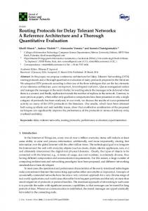
level progamming language, running on top of TinyOS operating system. Sensors are connected to the µC via I2C bus or SPI, depending on the version. For more details see [HiCu02, Hi03]. Mica2 and the Mica2Dust are the de facto standards in WSN research. MicaZ is the commercial version of the Mica platform manufactured by Crossbow Technologies [Cross]. The MPR2400CA board contains both microcontroller and radio, it just replaces the Mica’s CC1000 radio with a CC2420 (compatible with IEEE 802.15.4). The ATmega128L microcontroller runs MoteWorks from its flash memory. MoteWorks is based on the open-source TinyOS and provides reliable mesh networking, cross development tools, server middleware for enterprise network integration and client user interface for configuration and analysis. The board can be configured to run the sensor application and the network/radio communications stack simultaneously. The radio includes a hardware encryption module with AES-128. Crossbow offers a variety of custom sensor boards (with temperature, barometric pressure, acoustic, acceleration, seismic, etc. sensors) and data acquisition boards which can be easy connected to the MicaZ via a standard 51-pin expansion connector. Additionally, the connector supports analog inputs, digital I/O, I2 C, SPI and UART interfaces. When the MicaZ mote is connected to a standard PC interface it can operates as a base station allowing the aggregation of data onto a PC. Platform

Mica2 Berkeley Atmel ATmega128

Telos Berkeley TI MSP430

MicaZ Crossbow MPR2400CA ATmega128L

BTnode Bluetooth Atmel ATmega128L

ScatterWeb FU Berlin TI MSP430F1612

Wakeup time (µs) Voltage [V] Active Power [mW] Sleep Power [µW]

180 2.7-5.5 33 75

6 1.8-5.5 3 15

180 2.7-3.3 15-32 75

180 3.3 39 9900

6 2.7-3.6 54 36

Radio

Chipcon CC1000

Chipcon CC2420

MCU+Radio board

Zeevo ZV4002

Chipcon CC1020

Data rate [Kbps] Switch on time [ms] Frequency [MHz] Standard Range(out/in) [m]

76.8 2 433/868/915

250 0.58 2400 802.15.4 125/50

250 0.86 2400-2480 802.15.4 90/25

723.2 2400 Bluetooth 1.2 40/20

19.2/38.2 kbaud 868 ISM/SRD 103 /300

Sensors on board

-

-

-

1

2

Microcontroller

Table 2.4: Well known sensor node platforms and their characteristics.

Telos is the fourth generation Berkeley mote platform [PSC05], designed between 2003-2004 by graduate students at Berkeley and researchers from Intel, ETH-Zürich and TU Berlin. It is the successor of the Mica platforms [HiCu02] and is characterized by ultra-low power operation, ease of use, and robust hardware and software implementation [Po05-2]. Telos (new mote design built from scratch) is using a TI MSP 430 microcontroller due to its smallest power consumption in both sleep and active modes and to its fastest wakeup time of 5.8µs to switch from standby to active mode. Note also in Table 2.4 that the µC requires a minimal 1, 8V low voltage supply compared to 2,7V required by the ATmega 128 used in Mica platforms. Low voltage is important

Chapter 3

Medium access control in wireless sensor networks The previous chapter has showed how low-cost, small and autonomous sensor nodes can form large multi-hop networks in which the cooperating nodes overcome their inherent individual constraints (processing, memory and communication abilities) and are able to provide extensive services in the area of monitoring applications. Restricted node size implies low-power batteries which in turn lead to limited coverage and communication range for sensor nodes. Especially in monitoring applicatons a sensor network consists of a large amount of nodes in order to be able to successfully cover the area under observation. Low sensing ranges result in dense networks and therefore it is stringent to design proper mechanisms to coordinate the access of nodes to the shared communication medium. Medium Access Control (MAC) protocols solve exactly this task, they control and regulate the access of a set of sensor nodes to the shared medium in such a way that some application dependent performance requirements are satisfied. As we emphasized in the previous chapter wireless radio communication is error prone, has limited range and consumes a lot of energy. These characteristics force a cooperation between the sensor nodes to relay information, which heavily impacts on the lifetime of the unattended sensor network. Recall that, from the energy point of view, communicating one bit is equivalent to execute several hundred instructions. Therefore, for a resource constrained sensor node is very important that the protocol stack operates efficiently and all the layers making up the protocol stack are optimized toward the specific requirements of the application running on top of it. A lot of research in the field of sensor networks has been done to optimize the data link layer. Considering the OSI reference model, the MAC layer is considered as part of the second layer, the data link layer (DLL), and sits on top of the physical layer. Nevertheless, there is a clear separation of tasks between the MAC and the remaining part of the DLL. The MAC layer is responsible to access the shared communication medium (the ether), while the remaining parts of the DLL are mainly responsible for synchronization, error control and flow control. The performance of any WSN application depends significantly on the effectiveness of the MAC layer. The kind of traffic that a sensor network needs to sustain impacts not only on the design of the MAC protocol, but also on the design of the upper layers, especially the network layer. Therefore, the present work focuses mainly on two layers of the protocol stack, the MAC layer and the network layer. This chapter concentrates on the MAC layer while the next chapter is dedicated to the network layer.

53

3.4. DISCUSSION AND COMPARISON OF MAC PROTOCOLS

85

3.4 Discussion and comparison of MAC protocols We start with an overview of a chronological development of MAC protocols designed for WSNs, illustrated in Table 3.1. The list starts with year 2002 and is not pretending to be complete. MAC protocols for WSNs can be classified after several criteria. We consider that the main criterion is how the nodes organize access to the channel and that other criteria play a secundary role. Therefore, the comparison criteria are in order: the number of channels, the class to which the protocol affiliate, the notification method to inform the receiver, the sustained communication patterns and the adaptivity to changes (both in time or space/place). Year

Protocol

Comparison criteria: channel, class, Rx-notify, comm.pattern, adaptivity, time synch., cross-layer info

2002

STEM [STGS02] S-MAC [YHE02, YH03] Preamble sampling , LPL [Ho02, HiCu02]

2 (2 radios), contention, wakeup, all, good, no, no 1, slotted, listening, all, reduced, no (SYNC pkt), no 1, contention, listening, all, sensitive to variations in traffic rate and dense neighborhood, no, no

2003

Sift [JBT03] TRAMA [ROG03] T-MAC [vDL03] EMACS [NDHH03] B-MAC [PHC04] WiseMAC [HDER03]

1, contention, listening, all, good, no, no 1, slotted, listening, all, good, yes,no 1 channel, slotted, listening, all, good, no (SYNC pkt), no 1, frames, schedule, all, good, yes, no 1, contention, listening, all, good, no, no 1, contention (np-CSMA), listening, all, good, no, no

2004

DMAC [LKR04] LMAC [HoHa04] AI-LMAC [CHH04] CSMA-MPS [MaBo04] DSMAC [LQW04]

1, slotted (per-level), listening, convergecast, weak, yes, no 1, frames, listening, all, good, yes, no 1, frames, listening, all, good, yes,no 1, contention, listening (strobing), all, good, no, no 1, slotted, listening, all, good, no (SYNC pkt.), no

2005

SYN-MAC [WUT05] PMAC [ZRS05] Z-MAC [RWAM05]

1, synch. frames, listening, all, good (mobile) , yes, no 1, hybrid, listening, all, good (dense network), yes, no hybrid, knowledge of topology and loosely synchronized clocks

2006

X-MAC [BYAH06] SCP [YSH06] XLM [AVA06] 802.15.4 [IEEE15-4]

1, contention, listening(strobing), all, good, no, no 1, hybrid, listening, all, good, yes, no 1, contention, receiver-initiated, all, good, no, yes 1, slotted, listening/schedule, all, good, yes, no

2007

RMAC [DSJ07] Crankshaft [HaLa07]

1, slotted, listening, all, good, yes, yes 1, hybrid, schedule receivers, dense network, good, yes, no

2008

RI-MAC [SGJ08] Y-MAC [KSC08]

1, contention, receiver-initiated, all, good, no, no multi, frames (TDMA), listening, all, good (burst), yes, no

Table 3.1: Comparison of several MAC protocols for WSNs.

To have a better overview on the different protocols the Figure 3.25 illustrates also their chronological development within each class. This ”evolution” for each line will be the starting point for the following discussion and comparison of protocols as it naturally leads to the optimizations brought by each new

Chapter 4

Routing Routing is the task of finding a route or a path from a sender to a desired destination node. We start this chapter with a small introduction in routing and related problems, current research in the field and a review of some widely known routing protocols (used nowadays) in wired and wireless networks.

4.1 Overview of routing protocols 4.1.1 Wired networks In the wired world of the internet the routers are responsible for receiving and forwarding packets through the interconnected set of networks. The internet is dynamic, routes may change because some portions of the network may have failed or some parts of the network are congested. Here a router takes routing decision based on knowledge of the topology, delay and current traffic conditions. In order to be able to take the decision (which networks can be reached using which routes), routers exchange routing information using a special routing protocol. The routing information consists of some costs about the topology and delays of the network. Different approaches for finding routes between networks are possible. These approaches may be classified based on the type of information the routers need to exchange. Traditional known shortest-path routing algorithms are Distance-Vector routing (DV) [He88], [PeDa03], [Ta96], and Link-State routing (LS) [MRR80], [Ta96], [PeDa03]. • Distance Vector or the distributed Belmann-Ford (DBF) algorithm requires that each node exchanges information with its neighbors (directly connected in the same network). Each node maintains in its routing table a vector of link costs for each adjacent network. Each routing table entry - identifying a network entity (gateway or host) - includes the next-hop (gateway) and a distance metric (measuring the total distance to the entity) for that entity. The reception of a routing information packet containing a routing table entry for a destination implies that the receiver can route to that destination via the neighbor who sent that packet, at a cost equal to the sum of the distance in the routing table entry and the cost of the link over which the packet was received. The route for a destination propagates one hop each time the router sends the newly received route for that new destination. After some time, all nodes learn routes to all

93

4.2. ENERGY-AWARE ROUTING

133

isfying certain QoS metrics like delay, bandwidth, etc. Sequential Assignment Routing (SAR) described in [SGAP00] is one of the first protocols, where the routing decision depends also on the QoS on each path, besides energy and the priority level of each packet. Another QoS routing protocol for WSNs is SPEED [HSLA03], which provides soft real-time end-to-end guarantees.

SPIN [HKB99, KHB02] Directed Diffusion [In02] ACQUIRE [Sa+03] COUGAR prj.[YaGe02] EAD [BCL03] EAR [ShRa02] Epidemic Alg.[Ak+06] GBR [SS01] GRAB [YZLZ05] GAF∗ [XHE01] GeoTORA∗ [KoVa03] GEAR [YEG01] GPSR∗ [Ka00, KaKu00] Gossiping [HeLi88] HPAR [LAR01] LEACH [HCB00] MCFA [YCLZ01] PEDAP [TaKo03] PEGASIS [LiRa02] Rumor Routing [BrEs02] SAR [SGAP00] SPEED [HSLA03] TEEN [MaAg01] TreeCast [PDSJ04]

√ √

√ √ √ √

√ √ √

√ ! √

√

√ √ √ √

√ √

√ √ √ √ √

√

√ √1

√

√1 √1

√ √

√

√

√ √

√ √

√

√ √ √ √ √ √ √ √

∅

√ √

Limited applicability

Reliability mechanism

Data Aggregation

Energy-aware

Quality of Service

Multipath

Regular routing state

Sink-initiated

Source-initiated

Reactive

Proactive √

√ √ √ √

√ √

√ √ √

Node-centric

√ √ √ √ √ √ √ √ √

√

√ ! √ !

√ √

Data-centric

Location

Hierarchical

Routing protocols

Flat

Characteristics

√ √ √ √

√

√ !

√

√

√

√

†

√

√ √ √

√ √ √ √

∅

√

√ √ √ √ ∅

√ √

√ √ √ ! √ ! √ √

† √ √ √ √

† †

√

Table 4.2: Characteristics and comparison of routing protocols in sensor networks. (∗ designed initially √ √ for MANETs; 1 - one sink (special cases); ! - restricted support, † - restricted assumptions)

We summarize the protocols in Table 4.2, where the characteristics and properties of each routing protocols are indicated. These protocols comprehend several crucial design approaches and techniques for routing in WSN. We notice that the categories are not exclusive and only a few of the protocols are using energy-aware approaches. Moreover some of the protocols are not suitable at all since they make certain assumptions that are hard to realize. For example, PEGASIS assumes that each node is able to commu-

Chapter 5

Node Software Architecture This chapter presents our modular, energy-aware architecture for a sensor node aiming to improve composability and reusability of protocols modules at each layer of the protocol stack.

5.1 Motivation and objectives So far we notice in the literature an explosion of protocols for WSNs, mostly with a monolithic design and each making different assumptions about the network stack composition, thus having limited interoperability. The lack of an overall sensor network architecture is one of the primary factors limiting research progress in WSN [CDE+05]. According to [Po05] a response to this situation is a unifying abstraction proposal, called sensor protocol (SP), meant to provide more modularity to sensor node designs, thus regularizing assumptions about interfaces and enabling code reuse (see also [Po05-2, HSW+00]). The next step is given in [EFK+06], which implements and evaluates a modular network layer for sensor networks aiming to meet these goals. In our work we strive for a modular, energy-aware architecture for a sensor node aiming to improve composability and reusability of protocols modules at each layer of the protocol stack. Even though we focus on energy-efficient routing protocols the insights gained from the framework implementing our architecture reveals that a joint optimization of several protocols residing at different layers leads to better performance results. A wireless sensor network achieves the requirements of the application running on top of it (i.e., monitors the environment) as long as its constituent nodes are operating correctly. A node with depleted battery is not able to communicate and therefore it is useless for the network. Our main goal is to prolong the network lifetime by conserving the energy of the nodes as long as possible. The behavior of the nodes between source(s) and sink(s) depends on several factors such as the network topology and connectivity, the number of active requests in the network, the position of source(s) and sink(s), communication pattern, MAC protocol parameters (e.g., listen and sleep times), application parameters (e.g., interest refresh rate) and so on. The cumulated impact of such a large amount of parameters on the behavior of individual nodes is difficult to predict. For a ressource constrained sensor node is very important that the protocol operates efficiently and all the layers making up the protocol stack are optimized toward the specific requirements of the application running on top of it. In particular, the energy consumption should be optimized at each layer and the cooperation between layers should be

139

CHAPTER 5. NODE SOFTWARE ARCHITECTURE

146

from the application layer on gate upperIn is always forwarded to the output gate fromUpper to the FU. In this way the FU component recognizes that the packet is coming from the upper layer. In the opposite direction a packet from FU received by the IOU on the input gate toUpper is always forwarded to the application layer on the output gate upperOut. The same convention is used to forward packets from/to the lower layer as illustrated in Figure 5.4. • to assign the node’s identifier as source address to each outgoing network packet.

ruIn ruOut

Routing Protocol (code)

getNext() getAllNext()

Interface RU−FU

toUpper fromUpper

Layer

IO Unit

Neighbor Table nID avgRcvT

...

energy

register, manageTableEntries, get/setEntryFields, manageRUs ...

fwd to RU ackf

fromLower

inspectHeader localComputation manageNeighbor

mtype

Interest Table

ACK

...

Gradient Table

Resend−List

manageRetransmissions

FU−CR

Cross

toLower

Strategy Unit

fromLower

toUpper

Routing Unit

fromUpper

upperOut

upperIn

Application Layer

sendACK resend

yes

lowerIn lowerOut

...

toLower

updateHeader

ackf

Forwarding Unit Network Layer

Link Layer

message flow

cache updates

function call

Figure 5.4: Detailed interaction between the components of the network layer.

5.4.2 The Forwarding Unit The Forwarding Unit (FU) is the main component of the framework and glues the other components of the network layer together. Its main tasks (see Figure 5.4) are: • to inspect and update the basic part of the header for each network packet. For example, for each incoming packet from the lower layer it extracts relevant information such as the sender address and its energy or it computes the transmission time of the current packet (using a timestamp) in order to manage the Neighbor Table. For each outgoing packet the FU updates certain header fields, such as the packet’s sequence

Chapter 6

Framework design and implementation Our complete (prototype) architecture is implemented using the open source OMNeT++ 3.4b2 discrete event simulation package [OMNeT, Va06, Va01] and its Mobility Framework 2.0p3 [MF]. The framework offers support to build a complete protocol stack to simulate a wireless sensor node. In this chapter we describe the architecture implementation inside our sensor network framework, referred as SNF, discussing the main modifications and extensions that have been required in order to simulate a sensor node very close to reality.

6.1 The OMNeT++ simulator OMNeT++ is a C++-based discrete event simulation environment designed to support the simulation of (tele)communication networks, multiprocessors and other distributed and parallel systems. The motivation of developing it was to produce a powerful open-source discrete event simulation tool, available on all common platforms including Linux, Mac OS/X and Windows, that can be used by academic, educational and research-oriented commercial institutions. OMNeT++ tries to fill the gap between open-source, research-oriented simulation software (such as ns-2 [BBE+99] and expensive commercial alternatives (opnet [OPNET]).

6.1.1 Motivation for OMNeT++ OMNeT++ promotes a framework approach by providing the basic machinery and environment to build own simulations. Even though ns-2 is maybe the most widely used network simulator in academic and research, its goal consists of building a network simulator by directly providing simulation components for different communication networks. In contrast, OMNeT++ provides a platform, on which various research groups can build their own simulation frameworks, which lead to an abundance of OMNeT++based simulation models and model frameworks. Ns-2 lacks many tools and infrastructure components that OMNeT++ provides: support for hierarchical models, a graphical editor, graphical analysis tools, GUI-based execution environment (except for the network animator), separation of models from experiments, simulation library features, etc. Ns-2 concentrates more on developing the simulation models and much less on simulation infrastructure.

187

6.3. NEW FEATURES FOR THE SIMULATOR

203

The finalize method is called at the end of the simulation to record all scalar variable in the corresponding output scalar file by calling the OMNeT++ recordScalar method. We provide a script in order to parse the resulted huge statistical data files (the scalar and vector output files), to filter some nodes (especially for large sensor networks) and to plot these performance statistics. The script file calls the gnuplot program which plots the selected statistical data into a png or pdf file. For more details see Appendix A.2.

6.3 New features for the simulator In order to create a simulation network it is necessary to define in the configuration file the node coordinates either by assigning a fixed position or by leaving the simulator to place it automatically (random position). The automatic placement of nodes is very useful especially for large networks. The common way to generate a simulation network is a combination of fixed and automatic positioning. One starts to place some nodes at desired places and allows the remaining nodes to be placed automatically. In this way one has a minimal guarantee that the network is connected. Even then, the randomly placed nodes of the resulted network may be ununiformly distributed, i.e., some parts of the network are more densely deployed than other. If the achieved network connectivity is not appropriate, one needs to move some nodes from a dense part or to add new nodes into the network; for such cases, a ”drag-and-drop” facility in the simulation window saves a lot of time to position the nodes in the field. In the sequel we discuss a possibility to implement this and other features such as creation, deletion, disconnection and reconnection of nodes. The user interaction with the GUI generates an event that is caught by the OMNeT++ code. The ”action” that needs to be taken is provided in the Mobility Framework (MF) code (containing the implementation). For the drag-and-drop facility, the control flow starts in OMNeT++ code (the user drag-and-drops a node), continues in MF code (the node is moved to its new position, the communication topology is updated) and finally ends in OMNeT++ code (the GUI refreshed and the nodes’ coordinates saved in the configuration file). The challenge is to create no (compiler) dependency from OMNeT++ code to MF code. Since both code-extensions (to OMNeT++ and to MF) could be included in future new releases of the two packages we restrict ourselves to minimal changes of the original files (some OMNeT++ files had to be modified). Keeping this aspects in mind, we follow up the steps: 1) specify an extension section inside the OMNeT++ initialization file; 2) define additional controls (keys, buttons or submenus) with given functionality in the simulator window; 3) provide the required interaction between the OMNeT++ and the Mobility code. The first step creates a section in the initialization file with the role to enable and disable the new features and to initialize some simulation parameters. [ changenewdelete ] changenewdelete =yes

# enable the extended f e a t u r e s

In the second step we define some special keys, buttons and submenus. In order to move a node we define a special key combination (Ctrl-Mouse1) to trigger the movement of the node. To create a new node we add the New Submodule button and to delete, to disconnect or to reconnect node we define

Chapter 7

Simulation and Evaluation The ultimate goal of running a simulation is to provide results and to get some insight into the behavior of the sensor network by analyzing and evaluating the obtained results. In this section we describe the simulation environment and show simulation results that illustrate the possibilities of our framework in the context of energy-aware routing. One of the strengths of our framework is that one can execute the simulation under a powerful, customizable graphical user interface. The GUI makes the components of a simulation model fully visible to the user running the simulation: it displays the network graphics, highlights the routes followed by user-relevant messages, reflects the state changes of the nodes, animates the flow of messages and allows the user to inspect the objects and variables within the model. The WSN-customized facilities added to OMNeT++ help the user to deploy fast simulation scenarios, to identify easily the sink and sources, to inspect on-the-fly the node’s cache structures (by push of a button) and to change dynamically the network topology during runtime. All these are useful to check that protocols, strategies, etc. work as expected (conform with the specification) and to have a general view about what happens in the network. Usually simulation produces large amounts of raw data, which need to be organized in an appropriate way. The OMNeT++ provides the run concept, representing one instance of running the simulation, that allows to gather all relevant statistical data in one output file. Simulation results can be saved either in scalar or in vector output files. Output scalar files contain several output values, whereas output vector files contain several output vectors (time series: values with timestamps). In this way for each run the statistical results are individually saved in different files. Each time when we intend to compare some performance criteria, we say that we take a measurement by setting up several runs in the OMNeT++ configuration file. At the end of the measurement, we got all the output files1 that we need to plot the results (in order to evaluate and analyze them). Running the simulation with the graphical user interface enabled is a time consuming activity and therefore, is preferred to run the simulation as a command-line program. Moreover, the output files containing the simulation results are sometimes very large (proportional with the number of nodes in the network and the amount of statistical data under observation). Thus, analyzing the simulation results is also a time consuming activity. In most cases the user expects to see the same type of data for each run of the simulation and to draw/plot the same graphs (charts). In order to avoid repeating the steps of re-drawing the graphs every time a simulation has to be rerun for some reason, we automatize this process by writ1

This files have the extensions sca and vec

209

CHAPTER 7. SIMULATION AND EVALUATION

210

ting a script2 that is able to process, filter and automatically plot each of the statistical result from the output simulation files.

7.1 Simulation environment and parameters setup General simulation assumptions: • The sensor nodes are assumed to be static and randomly distributed in a two-dimensional plane. The nodes are bulding a connected multi-hop network. • Nodes are considered interchangeable, each one having a single radio, but equipped maximal with three arbitrary sensors. • All nodes have the same transmission range. A link between two nodes in the network graph exists if the nodes are within their communication range. We have chosen the transmission power in all test networks so that a node has at most 8 neighbors. • The sink(s) can be randomly chosen. The interest specifies the type of data requested and additionally the area of the network under observation. The source nodes are identified according to the interest. • At the beginning of the simulation each sensor node has a given initial energy available. The energy consumption model is configurable to current hardware characteristics. The current settings are given in the next subsection. • Collisions are recognized by the implemented MAC protocols and node and link failures are simulated during run-time. • Depending on scope of the simulation the parameters of each layer of the protocol stack must be appropriately configured. • We use as test network for a preliminary simulation a sensor network with 48 nodes. Later we increase the number of nodes and use test networks with 130, 250 or more nodes or special networks to illustrate some interesting aspects.

7.1.1 Preliminary simulation setup Configuration of the parameters: The following settings are generally valid excepting the cases where explicit configuration parameters are either mentioned or required. • The simulation time is usually fixed to 5 minutes (in some few scenarios 2min). The simulation is configurable to stop also after a given number of data packets. • The data generation rate is specified by the interest and varies from high (data generation interval of 50ms) to low traffic (data generation interval of 5s). In the simulations the standard data interval is 200ms (where all MAC protocols operate correctly). It is assumed that during the simulation time the interest does not expire. 2

the scalars and plove programs provided by OMNeT++ at that time have been rudimentary

7.1. SIMULATION ENVIRONMENT AND PARAMETERS SETUP

211

• The interest is injected (by the sink) in the network at 2s from the start of the simulation and it is refreshed usually in a 5s interval. The target area can be restricted by the interest. • Interest (or refresh) messages are transmitted as a broadcast and data messages as unicast. • The energy at startup is set to 50.000 mJ. The energy consumption model is the one presented in §6.2.5, where the radio power to transmit and to receive are 32 mW and 12 mW, respectively; in idle mode 10 mW and in sleep mode 50 µW. Since at this values the simulation time is long until the energy decreases visible we used a scaling factor of 10. The CPU needs 7 mW and 5 µW in active and sleep mode respectively. • The radio switch time from receive to send or viceversa is set to 2ms (the switch time to sleep state is 0). The standard radio bit rate is set to 1 Mbps. We chose for our simulations a network with 48 nodes as our standard test network, with one sink (node 21) and one source (node 16). Figure 7.1 illustrates the network (before the simulation starts) to allow the reader to identify easily the nodes referred in the text since the later snapshots are relatively small. As can be seen the shortest path between source and sink consists of 6 hops and there are several paths from source to sink.

Figure 7.1: The standard network with 48 nodes used in most simulations.

7.1.2 Goal of the measurements We measure the energy consumption at each node by automatically recording3 the time spent by the radio in different states. The power consumption in a battery powered node can be divided in power needed for communication and power needed for non-communication activities. The first one is specified 3

we don’t call explicitly functions to compute the energy


212

by the radio activity and depends on the amount of traffic transmitted and received by the node. The second one is specified by the activities that the µC performs as a result of radio operations (copy and buffer messages) or protocol operations (in-network processing, aggregation). We suppose that the power consumed for non-communication activities is fixed (configured correspondingly to the actual hardware used) and depends only on the number of bytes that are processed. First we compare the energy performance of several MAC and routing protocols under optimal configuration with periodic, known traffic. For static traffic loads we can optimize the protocols for energy conservation. Then we configure scenarios with unknown or unpredictable traffic (various data rate, different bit rate, variable number of sources and sinks, etc.) and stress the nodes to operate from optimal regime to their limits. At the end of each simulation we illustrate the energy consumed by the nodes (individually or globally), analyze and discuss the results. The simulation results are grouped in two categories: those resulted by the comparison of MAC protocols (where the routing protocol is considered fixed) and those resulted by comparing different combinations of routing protocols with MAC protocols. Based on the insights gained from the simulation results, we derive guidelines for energy efficiency and design improvements.

7.2 Comparison of different MAC protocols In order to compare different MAC protocols, we assume that the layers above the MAC layer are the same. In other words, we keep the same application and routing protocol4 in our protocol stack; the only module that changes in the simulation framework is the NIC module. By the comparison of MAC protocols we analyze the following performace criteria: the energy consumption (to predict the network lifetime), the ability to avoid collisions, the latency achieved by the source-sink communication, the protocol overhead and the maximal throughput. We point out the limitation of each MAC protocol (the point where it collapses) and illustrate the impact of the data rate and bit rate on the energy consumption. Parameter

S-MAC

Listen time [ms] Frame time [ms] Overhearing avoidance Packet length [Bits]

60 600 enabled 472+128+72

MAC protocols T-MAC B-MAC 15 600 enabled 472+128+72

0.05 5 472+128+192

802.11 472+128+72

Table 7.1: MAC protocol specific parameters configuration. It is assumed a network packet length of 472 Bits (including the header of the application and network layers).

Besides the above general settings each MAC protocol has particular parameter settings. MAC implementations have many specific design parameters, which have impact on performance. Since those details could distract us from the main task of comparing the MAC protocols, we restrict ourselves here to the main one (for the rest see Appendix) as illustrated in Table 7.1. 4

we deliberately consider here only the hc strategy since the route selection (first shortest path found) is relatively stable.

7.2. COMPARISON OF DIFFERENT MAC PROTOCOLS

219

7.2.7 Estimation and conclusion An overview of the result of comparing the set of the four MAC protocols is illustrated in Table 7.3:

Energy consumption (low data rate) Energy consumption (medium data rate) Energy consumption (high data rate) Collisions Discarded frames Latency

T-MAC

S-MAC

B-MAC

802.11

++ ++ + o + −−

o o o + −−

+ (+ + +∗ ) o o ++

−− −− ++ ++ +++

Table 7.3: Comparison between the four MAC protocols. ( ∗ =appropriate configuration of the B-MAC parameters under the assumption of an adaptive, energy-aware routing protocol).

T-MAC can be characterized as a flexible and energy-efficient MAC protocol, which achieves good results for various data rates (at the expense of a reduction in peak throughput). The only drawback remains its latency with high standard deviation. From the programming point of view the overhead to synchronize the nodes must be mentioned. S-MAC is less flexible than T-MAC and has the same drawback as T-MAC concerning the latency. SMAC requires an appropriate configuration of its parameters. For application scenarios where the data rate is relatively constant (and known), the parameters can be manually adjusted such that the highest data rate case (worst-case analysis) is covered. Since its duty cycle is fixed (for all nodes) often a rather large value must be selected to avoid discarding packets under peak loads, which causes S-MAC’s behavior to deteriorate for increasing traffic loads. The energy consumption of S-MAC is relatively constant and depends mainly on its duty cycle. Various data generation rate and bit rates have no relevant impact on the energy consumption. Its main drawback remains its inadaptability to fluctuating data traffic. B-MAC does not sustain so high data rates as T-MAC and it is recommended for applications where the data traffic is medium or low. In this case the energy consumption is also low, especially when the routing protocol above the MAC adaptively changes the route according to the residual energy of nodes (see §7.2.1). The source-sink latency is also low (with a small standard deviation) and can be ahead predicted. From the programming point of view the implementation is simpler than in case of S-MAC and T-MAC (the active-sleep regime of nodes is not synchronized), but requires an optimal configuration of the parameters. WLAN 802.11 has the main drawback in its high energy consumption. As can be seen the analyzed MAC protocols have different advantages and disadvantages. The configuration of the parameters of each MAC protocol have a huge impact on their performance. Therefore, it is advisable to analyze the application requirements and then choose the appropriate MAC protocol. As described in Chapter 1 the range of applications is wide and the requirements can be very different. The main conclusion is that the MAC protocol has a huge impact on the energy efficiency and the latency of the whole application that embeds the MAC protocol. The MAC protocol is responsible to achieve a low energy consumption. Only when a significant difference in consumption between communicating and not communicating nodes exists, can a routing protocol, which provides adaptive and flexible routes, to prolong significantly the life of the entire network.


220

7.3 Comparison of different routing protocols To illustrate the performance results of different routing protocols (used in WSN) we start with the one described in §5.7. Recall that this routing protocol is based on two phases: the interest propagation and the data event gathering. The routing protocol can be configured to use several strategies. The ultimate goal of the protocol is to illustrate the benefit of strategies that balance the load of forwarding the data packets on all the nodes and keep the energy consumption low. The main objective of the following simulations is to analyze the impact of several routing strategies on the energy consumption of the nodes. In a ”network-lifetime” scenario we illustrate comparatively the impact of the hc and hccE strategies on the nodes’ depletion time when using T-MAC as a MAC protocol.

7.3.1 Simulation setup for routing In order to build a complete routing protocol we benefit from the plug-and-play facility of our architecture. We configure the protocol stack by plug-in first the T-MAC protocol layer and keep the application layer and network layer unchanged. The simulation network is the same one used by the MAC protocol comparison with 48 sensor nodes. The configuration of the main8 parameters is divided on the layers of the protocol stack. At application layer: • Simulation time is set to 5 minutes.

• The sink is node 21 and injects an interest with the following data attributes: – Data generation interval is set to 200 ms. – Requested data is temperature in the zone of node 16. – The interest is valid for 5 minutes and is refreshed at a 5s interval.

At network layer: We setup the simulator with four different strategies: • The first strategy was to route the data packets on the shortest path between source and sink, referred as the hop count (hc) strategy. • The second strategy combines the hop count metrics with the neighbor residual energy, referred as the hc&E strategy. • The third strategy, referred as the hc&cE uses (besides the hc) instead of residual energy E the critical energy (cE), i.e. the least residual energy on the path between the sink and source. Each node u computes cEu = min{Eu , max{cEv |v ∈ N eighbor(u) ∧ hcv ≤ hcu }} and piggybacks its local residual energy to each packet sent (§5.7.7.3). • A fourth strategy uses a combined metrics involving both the hop count and the critical energy. Each node computes and forwards the pair: [ hop count distance to sink ; critical energy on path], as [hcu ; cEu ] = [hcv ; cEv ] ⊕ [1; Eu ], where [hcv ; cEv ] is min{hcv /cEv |v ∈ N eighbor(u)} and the operator ⊕ is defined for each term as hcu = hcv + 1 and cEu = min{Ev , Eu }. This strategy is referred as the hccE strategy. 8

we restrict ourselves here only to the most important ones

7.3. COMPARISON OF DIFFERENT ROUTING PROTOCOLS

221

We setup four different runs each one corresponding to a different routing strategy. At link layer: We use • T-MAC: Listen time is set to 30 ms and the frame time to 600 ms. All other parameters (concerning the energy consumption, radio bit rate, radio switching times, etc.) are left unchanged (as given in §7.1.1).

7.3.2 Impact of the routing strategy on the energy consumption of nodes Simulation results for the impact of the four routing strategies on the energy consumption are given in Table 7.4. network with 48 nodes

hc

hc&E

hc&cE

hccE

Energy consumed

(hop count)

(energy)

(critical energy)

combined

Max [mJ]

5.520

4.973

4.402

4.935

Max-Min [mJ]

3.625

3.077

2.507

3.038

Std. dev.[mJ]

1.140

980

797

989

Total [mJ]

145.689

149.962

150.557

148.769

Table 7.4: Impact of routing strategies on the energy consumption.

As can be seen there, an energy-aware approach leads to a better overall behavior of the network. More precisely, the results show that the best metrics are combinations of hop count with critical energy (last two strategies); hereby the overall energy consumption is slightly larger but the consumption is better balanced among nodes, which extends the network lifetime. When using only the hop count metrics we notice a very unbalanced energy consumption of the nodes (see standard deviation, the difference Max–Min); nodes on minimal hop count paths will soon be depleted while nodes with enough energy on comparable paths are not employed at all). Figure 7.14 illustrates the sorted energy consumption of all nodes using T-MAC protocol with all the four strategies given before. The energy is sorted in order to better visualize the distribution of the energy consumption on the nodes.

Figure 7.14: Energy consumption using different routing strategies (with T-MAC).

One can notice here that strategies 3 and 4 using both the hop count and critical energy have the positive effect that they balance the overall energy consumption on more nodes. This can be observed by com-

7.3. COMPARISON OF DIFFERENT ROUTING PROTOCOLS

225

7.3.4 Impact of the routing strategy on the source to sink latency Interesting is also to compare the source-sink latency for both strategies. We illustrate comparatively the source to sink latency with aggregation enabled in Figure 7.20 As expected, the source-sink latency in the case of the hccE strategy increases on one side since due to the load balancing policy data packets travel along longer paths (is maximum one frame time longer 0.6s) and on the other side due to the underlying T-MAC.

Figure 7.20: Source to sink latency for the hc (left) and hccE (right) strategies.

Moreover, we can also plot the latency or the number of collisions on each node, as well as the MAC queue length. For space reasons we omit them here (see §A.3).

7.3.5 Cumulative impact of the broadcast delay and strategy on the energy We illustrate further the impact of the broadcast delay (Tw ) on total energy consumption. As described in §5.7.4 it would be expected that for longer Tw the energy would decrease. This is true for MAC protocols without or with a fixed active-sleep regime. Is it true also for T-MAC? Adjusting Tw to achieve a better energy consumption remains difficult and we give some results for simulations configured with T-MAC. Nevertheless, the cumulative impact of different link (MAC, radio), network and application parameters should be further studied/analyzed to find out if an optimal value for Tw exists. Since we set the listen time and frame time for T-MAC to 30ms and 600ms respectively, we run the simulation for three different values for Tw : 0.4ms, 20ms and 600ms. Why this times? The simulation results for hc and hccE strategies are given in Table 7.5. The simulation time was 2min and each of the 3 sources generates 5 data packets/s. Energy [mJ] Strategy

Broadcast delay (Tw ) 0,4ms

20ms

hc hccE

85.403 91.868

84.759 89.964

600ms

Rebroadcasts Strategy

0,4ms

20ms

600ms

85.221 90.964

hc hccE

1.067 (2) 1.534 (2)

1.053 (4) 1.268 (0)

1.052 (4) 1.063 (1)

Table 7.5: Impact of Tw on energy consumption.

Broadcast delay (Tw )

Table 7.6: Impact of Tw on number of rebroadcasts.

The best energy consumption is achieved with a broadcast delay of 20ms, thus not for the highest value of Tw . In order to count how often each node rebroadcasts an interest we stop the refreshes after 112s (the simulation runs until 120s). In this way, we guarantee that each interest refresh reaches all the nodes (no

Chapter 8

Conclusions This chapter summarizes the results from the previous ones and gives a brief outlook on possible future research directions.

8.1 Accomplishments and contributions The main contributions of the thesis are: • We designed and implemented the network architecture of a sensor node, taking into account the energy consumption of each of its components. The architecture has a modular structure, promoting composability and reusability of protocols modules at each layer of the protocol stack. • For routing protocols we proposed new strategies (metrics) taking into account energetic information enabling us to take appropriate routing decisions in order to extend the lifetime of the WSN. Besides providing energy-efficient MAC protocols and routing protocols independently, we also ensure a joint optimization by enabling an additional exchange of relevant information between the two protocols by adding a cross-layer component in the protocol stack. • We developed a (modular) simulation framework which provides a flexible approach to design and plug-and-play various protocols at network and MAC layers, and to combine and analyse the impact of different strategies and others factors on performance and lifetime of the WSN. The framework can automatically visualize performance criteria to enable a fast evaluation and comparison of protocols. Further contributions include: • We have studied the characteristics and evaluated the capabilities of the new communications standards and technologies (such as range of communication, power consumption characteristics, etc.) and gave preliminary hardware design considerations for own defined and pre-designed sensor nodes. • We proposed a general model for the energy consumption of a node (independent of the application) and also a model for the sensor network using only general assumptions about the node and the network.

241

242

CHAPTER 8. CONCLUSIONS • We analyzed and compared the current advanced techniques and algorithms for MAC protocols, highlighting their advantages and disadvantages, as well as their applicability. We also illustrated the operating mode of several low duty-cycle MAC protocols (S-MAC, T-MAC, Preamble Sampling) using state transition diagrams. • We implemented these MAC protocols and included them in our final software sensor node architecture. • We classified and compared existent energy-aware routing protocols; moreover we improved directed diffusion protocol as far as energy consumption is concerned. • Besides energy-aware metrics we considered also geographical approaches and in-network processing as useful mechanisms to improve the energy-efficiency of routing. • Since reliability in sensor network plays an important role we investigated different mechanisms to improve the robustness to different kinds of (node and link) failures and analyzed the trade-off between energy and robustness. • We illustrated in detail several approaches to maximize the lifetime of the WSN such as: flowbased modeling, max-min optimization and lifetime prediction techniques. Moreover, we discussed theoretical aspects and the NP-hardness of the problem and proposed a heuristic. • We proposed and compared several energy-aware routing metrics: hc&E, ∆hc/E, hc&cE and the corresponding distributed algorithms. We also introduced a more general and flexible approach for a maximum lifetime heuristic and gave the corresponding algorithm. • Our simulation framework offers, among others, the following facilities: – An energy component that models automatically the energy consumption in a sensor node. – A statistics component with automatic visualization of relevant data, which enables a fast analysis of different performance criteria. – Support for collision detection to consider the energy consumption due to collisions (in order to have a realistic energy model). – Drag-and-drop facilities and smart features to easily create, modify and reconfigure the network topology at startup and during runtime. These features includes creation, deletion, disconnection, reconnection and movement of nodes. Moreover, we integrated a userFunction, which can be mapped to any utility function related to a node. – Improvement of the GUI visualization by customizing it to WSN (e.g. route color schemes, node highlight effects and animation, etc.). – A debug level activation scheme which allows to stop the simulation at deliberately chosen execution points without recompiling the huge source code. • We provided and evaluated many simulation results under different assumptions for various scenarios. Moreover, we gave some guidelines about which strategies, metrics, or even protocols are better suited for which category of sensor network applications.

8.2. FUTURE RESEARCH

243

8.2 Future research Our first goal for future work is to port the architecture implementation on real sensor network platforms, to validate and further develop the proposed models (energy, radio, network, etc.). Furthermore, the results obtained so far motivate us to continue and to extend the developed framework simulator. Here we will follow several directions: • To quantify the programming overhead needed to develop and integrate new protocols. • Since the MAC protocol has the main impact on the energy consumption, we intend to provide more MAC protocol implementations and to compare their performance. Carrying out comparative analysis between different MAC protocols and their interaction with network layer protocols will reveal surely other promising aspects that can bring optimization at both layers. • Bring more modularity at MAC layer: embed at MAC layer more customizable services like the receiver-based contention (or other innovative ideas from new MAC protocols), which in our opinion gives another perspective to the interlayer communication and would improve the energy efficiency of routing. • Extend the routing decision spectrum by providing at network layer, besides reliability and timecritical services, additional ones like congestion control, route provision with resource reservation, etc. This can be achieved using information available at the application layer. • Develop further routing algorithms and investigate additional in-network processing (aggregation, compression) algorithms. Moreover, we have started to design routing protocols for mobile scenarios, where nodes are allowed to move. • Radio communication links are known to have transitional region with widely varying degrees of packet loss and high error rates. There might be cases where distant nodes may have smaller loss than nearby nodes. In terms of energy, it might be more efficient to establish longer paths exhibiting low loss instead of shorter ones with poor link qualities where more energy has to be spent for successful packet delivery (due to retransmissions). For such cases new metrics are required that should incorporate besides the energy cost the rate of successful delivered packets and/or the link asymmetry attributes. • The graphical runtime environment, provided by the OMNeT++ 3.4b and used during the present work, allows the user to follow the interaction between by slowing down the animation or running the simulation in single-step mode. To catch the exact sequence of events or to capture the timing relationships between several events was hard. The OMNeT++ 4.0 simulation kernel is capable of logging (in file) various events during the simulation. The file can be later processed by a sequence chart diagram tool in order to analyze and display the causes and effects of an event. This could be a very useful tool, after porting the current implementation to OMNeT++ 4.0, to find explanation for results of simulation scenarios that could not be explained.

244

CHAPTER 8. CONCLUSIONS

Appendix A

Configuration parameters A.1 NIC layer (includes MAC) A.1.1 Icons to visualize the node state The following icons are used to visualize the node state (according to the radio state) during the simulation: Start state: for protocols with an active-sleep regime no schedule active (S-MAC, T-MAC). Node active. Radio in idle-receive mode. Node just receives data. Node sends data. Sleep state. Switch state. Radio switches to receive or send. Not defined state (state unknown).

A.1.2 NIC parameters MAC layer parameters: (S-MAC, T-MAC and B-MAC) listenTime Time interval (in [·10−6 s]) for which the node is active. This time must be at least at least 1.5 times the RTS contention time. frameTime Frame length (in [·10−6 s]).

245

246

APPENDIX A. CONFIGURATION PARAMETERS

queueLength MAC queue length. The just processed frame is not considered. bitrate Known bit rate at MAC layer (must have the same value set for radio). defaultChannel Radio channel. headerLength MAC header length (in bytes). This is specific to each MAC. busyRSSI Threshold value to indicate a busy channel. airFrameHeaderLength AirFrame header length (must have same value set for physical layer). flags Specific T-MAC flags: 1=overhearing avoidance enabled (During NAV timer the node goes to sleep; 2=FRTS enabled; 3=both options enabled. dbgLL Global debug level for NIC. We introduced this debugging facility in order to be able to insert breakpoints in code without recompilation. One can enable simultaneously more debug levels (by simple addition). Physical layer parameters: transmitterPower Transmitting power of the radio. Influence the network topology. carrierFrequency Carrier frequency (needed to calculate the wave length). pathLossAlpha Channel (path) loss coefficient. thermalNoise Thermal noise on the channel (default: -100 dBm). The noiseLevel variable is initialized to the thermalNoise. When receiving a packet the physical layer module updates the noise level of the channel. Based on the packet’s receive power it is either further processed and handed to upper layers or just treated as noise. sensitivity Radio sensitivity defines up to what power level (in dBm) a packet can be understood. If the level of a received packet is lower, it is only treated as noise (default: -85 dBm). headerLength Airframe length (must have same value as AirFrameHeaderLength in MAC). publishRSSIAlways Flag to publish the RSSI. snrThresholdLevel SNR threshold level (in dBm). When a packet contains an SNR level higher than snrThresholdLevel it will be considered as lost. This parameter has to be specified at the beginning of a simulation. debug Debug to switch on/off the output of EV Radio component’s parameters: swSleep Switch to sleep time (in [s]). swSend Switch to send time (in [s]). swRecv Switch to receive time (in [s]). debug Debug switch.

A.2. THE SCRIPT TO PLOT STATISTICS AND SIMULATION FILES

247

A.1.3 MAC integration in simulator To embed a new NIC (including MAC) into a node protocol stack: 1. Copy the complete nic directory in the framework directory. 2. Edit the node’s protocol stack description file, SNFHost.ned, to change the nic module description file (to embed the new code). For example, to use the T-MAC (assuming that its description file is NicTMac.ned) one needs to change two lines: import ... // include code for each module ”NicTMac”, ... module MyHost parameters: ... gates: ... submodules: ... nic: NicTMac; display: "b=32,30;p=60,166;i=icon_nic"; // new icon ... connections: ... display: ... endmodule

3. Adjust the TMac.ini file to your application requirements (especially the frameTime, listenTime and queueLength configuration parameters).

A.2 The script to plot statistics and simulation files The script file plotstat sh requires the gnuplot program (at least version 4.2). In order to use the script just run it without arguments and the usage message will be displayed. In its simplest form the script requires two command-line parameters: the first one specifies the type of requested statistical data ( energy, latency, etc.) and the second one enumerates the nodes (their index) for which the statistic is required. Having the filtered data the script analyses the values, scales the x and y-axis scales (attaches a label to them) and generates, using the gnuplot program, the graphical representation either in a pdf file (the OUTPUTFILE argument) or in a separate png file. For example, to plot the energy consumption at nodes 1 3 7 21 in a pdf output file use: plotstat_sh --cenergy --pdf --hosts 1 3 7 21

A.3 Simulation files For the complete statistic data files obtained during different scenarios or different graphics please contact the author at the following e-mail [email protected].

APPENDIX A. CONFIGURATION PARAMETERS

248

A.4

Software used

In this work the following software packets were mainly used: openSuSe 11.0 (operating system), OMNeT++ vers. 3.4b2, Mobility Framework 2.0p3 and g++ version 4.3.1 (for the implementation of the simulator), doxygen 1.5.5 (for code documentation), latex and xfig graphic package (for the elaboration of the thesis and drawing the figures), dia version 0.96 diagram drawing program (for UML diagrams and sequence diagrams) and gnuplot 4.2 (for plotting the simulation results given in Chapter 7).

A.5

SNF with new features enabled New features

Drag−and−drop with Ctrl+MouseButton1 on node

New node

source area

Disconnected node

sink

Figure A.1: Simulator enhanced main window. Snapshot taken during a scenario with node 21 as sink and three sources inside the rectangle, using the first routing protocol with the third metrics. Data packets flow toward sink as indicated by the red arrows.

Bibliography [Ab70] N. Abramson: The Aloha system - Another alternative for computer communications, AFIPS Conference Proc., Vol.36, pp.295-298, 1970. [Ab85] N. Abramson: Development of ALOHANET, IEEE Transactions on Information Theory, Vol.31(2), pp. 119-123, 1985. ¨ Ulusoy, U. Çetintemel: A comparison [Ak+06] M. Akdere, C. Bilgin, O. Gerdaneri, I. Korpeoglu, O. of epidemic algorithms in wireless sensor networks, Computer Communications 29, pp.2450-2456, 2006. [AkYo05] K. Akkaya, M. Younis: A survey of routing protocols in wireless sensor networks, Elsevier Ad Hoc Network J. 3/3, pp. 325-349, 2005. [AlKa04] J.N. Al-Karaki and A.E. Kamal: Routing techniques in wireless sensor networks: a survey, IEEE Wireless Communications Magazine, Vol.11(6), pp.6-28, 2004. [Atm07] http://www.atmel.com/dyn/resources/prod documents/doc2467.pdf (last access 27.11.2007) [Atml07] http://www.datasheetcatalog.com/datasheets pdf/A/T/M/E/ATMEGA128L.shtml (last access 27.11.2007) [ACFP06] G. Anastasi, M. Conti, M. Di Francesco, A. Passarella: An adaptive and low-latency power management protocol for wireless sensor networks, in Proc. 4th ACM Int. Workshop on Mobility Management and Wireless Access, pp.67-74, Terromolinos, Spain, 2006. [ADT04] J. Alonso, A. Dunkels, T. Voigt: Bounds on the energy consumption of routings in wireless sensor networks, in Proc. 2nd Int. Workshop on Modeling and Optimization in Mobile Ad Hoc and Wireless Networks, pp. 62-70, Cambridge, 2004. [ALR03] J. Aslam, Q. Li, D. Rus: Three power-aware routing algorithms for sensor networks, Wireless Communications and Mobile Computing, Vol.3(2), pp. 187-208, 2003. [AMO93] R.K. Ahuja, T.L. Magnanti and J.B. Orlin: Network Flows: Theory, Algorithms and Applications, Prentice Hall, ISBN 0-13-617549-X, 1993. [ASSC02] I.F. Akyildiz , W. Su , Y. Sankarasubramaniam, E. Cayirci: Wireless sensor networks: a survey, Computer Networks: The International Journal of Computer and Telecommunications Networking, Vol.38(4), pp. 393-422, 2002.

249

250

BIBLIOGRAPHY

[AVA06] I.F. Akyildiz, M.C. Vuran, O.B. Akan: A cross-layer protocol for wireless sensor networks, Proc. Annual 40th Conf. on Information Science and Systems (CISS’06), pp. 1102-1107, Princeton, NJ, 2006. [Be06] J. Beutel: Fast-prototyping using the BTnode platform, in Proc. Conf. on Design, Automation and Test in Europe, pp. 977-982, Munich, Germany, 2006. [BrEs02] D. Braginsky, D. Estrin: Rumor routing algorithm for sensor networks, in Proc. 1st ACM Int. Workshop on Wireless Sensor Networks and Applications, pp. 22-31, ACM Press, Atlanta, 2002. [BCL03] A. Boukerche, X. Cheng, J. Linus: Energy-aware data-centric routing in microsensor networks, Proc. 8th ACM International Workshop on Modeling analysis and simulation of wireless and mobile systems (MSWiM), pp. 42 - 49, San Diego, California, USA, 2003. [BBE+99] E. Bajaj, L. Breslau, D. Estrin, K. Fall, S. Floyd, P. Haldar, M. Handley, A. Helmy, H. Yu: Improving simulation for network research, University of Southern California. http://eprints.kfupm.edu.sa/45347 (last access 2006). [BDSZ94] V. Bharghavan, A. Demers, S.Shenker, L. Zhang: MACAW: A media access protocol for wireless LANs, in Proc. SIGCOMM Conf., pp.212-225, London, U.K., 1994. [BHE06] M. Busse, T. Hänselmann, W. Effelsberg: Energy-efficient forwarding schemes for wireless sensor networks, in Proc. IEEE Int. Symp. on World of Wireless, Mobile and Multimedia Networks (WoWMoM), pp.125-133, Buffalo, New York, USA, 2006. [BKM+04] J. Beutel, O. Kasten, F. Mattern, K. Römer, F. Siegemund, L. Thiele: Prototyping wireless sensor network applications with BTnodes, in Proc. 1st European Workshop on Sensor Networks (EWSN’04), Vol. 2920 of Lecture Notes in Computer Science, pp.323-338, Springer, Berlin, 2004. [BMJ+98] J. Broch, D.A. Maltz, D.B. Johnson, Y. Hu, J. Jetchev: A performance comparison of multihop wireless ad hoc network routing protocols, in Proc. 4th Annual ACM/IEEE Int. Conf. on Mobile Computing and Networking (MobiCom 98), pp. 85 - 97, Dallas, Texas, USA, 1998. [BTn3] BTNodes - A distributed environment for prototyping ad-hoc networks, Web page ETH Zürich, http://www.btnode.ethz.ch/Documentation/BTnodeRev3HardwareReference (last access 12.2007). [BYAH06] M. Buettner, G. Yee, E. Anderson, R. Han: X-MAC: A short preamble MAC protocol for duty-cycled wireless networks, in Proc. 4th ACM Conference on Embedded Networked Sensor Systems (SenSys’06), pp.307-320, Boulder, CO, 2006. [CaKi02] J. Cano, D. Kim: Investigating performance of power-aware routing protocols for mobile ad hoc networks, International Mobility and Wireless Access Workshop (MobiWac’02), pp. 80, 2002. [CaWo03] A. Carzaniga, A.L. Wolf: Forwarding in a content-based network, Proc. ACM SIGCOMM 2003, pp.163-174. Karlsruhe, Germany, 2003. [Ch79] V. Chvatal: A greedy heuristic for the set-covering problem, Mathematics of Operations Research, Vol.4, pp.233-235, 1979. [ChGe98] T. Chen, M. Gerla: Global State Routing: A new routing scheme for ad-hoc wireless networks, in Proc. IEEE ICC’98, pp. 171-175, Atlanta, GA, 1998.

BIBLIOGRAPHY

257

[KaWi09b] A.F. Kacso, R. Wismüller: Modeling and simulation of multihop routing protocols in wireless sensor networks. To appear in Proc. 5th Int. Conf. on Wireless and Mobile Communications (ICWMC’09), Cannes, France, 2009. [KaWi05] H. Karl, A. Willig: Protocols and Architectures for Wireless Sensor Networks, ISBN: 978-0470-095102, John Wiley & Sons, 2005. [KoVa98] Y.B. Ko, N.H. Vaidya: Location-aided routing (LAR) in mobile ad hoc networks, in Proc. 4th Annual ACM/IEEE Int. Conf. on Mobile Computing and Networking (Mobicom ’98), pp.66-75, Dallas, USA, 1998. [KoVa99] Y.B. Ko, N.H. Vaidya: Geocasting in mobile ad hoc networks: Location-based multicast algorithms, in Proc. 2nd IEEEE Workshop on Mobile Computing Systems and Applications (WMCSA), pp.101-110, New orleans, USA, 1999. [KoVa00] Y.B. Ko, N.H. Vaidya: Location-aided routing (LAR) in Mobile. Ad Hoc Networks, ACM Wireless Networks Journal, Vol.6(4), pp.307-321, 2000. [KoVa02] Y.B. Ko, N. H. Vaidya: Flooding-based geocasting protocols for mobile ad hoc networks, Mobile Networks and Applications, Vol.7(6), pp.471-480, 2002. [KoVa00a] Y.B. Ko, N. H. Vaidya: GeoTORA: A protocol for geocasting in mobile ad hoc networks, in Proc. 8th Int. Conf. on Network Protocols (ICNP), pp. 240-250, 2000. [KoVa03] Y.B. Ko, N. H. Vaidya: Anycasting-based protocol for geocast service in mobile ad hoc networks, Computer Networks, Vol.41(6), pp.743-760, 2003. [KuAr04] S. Kulkarni, M. Arumugam: TDMA Service for Sensor Networks, in Proc. 24th Int. Conf. on Distributed Computing Systems Workshops - W5: ADSN (ICDCSW’04), pp.604-609, 2004. [KAB+05] L. Krishnamurthy, R. Adler, P. Buonadonna, J. Chhabra, M. Flanigan, N. Kushalnagar, L. Nachman, M. Yarvis: Design and deployment of industrial sensor networks: Experiences from the north sea and a semiconductor plant, in Proc. 3rd ACM Int. Conf. on Embedded Networked Sensor Systems (SenSys), pp.64-75, San Diego, USA, 2005. [KAT05] [8] A. Koubâa, M. Alves, E. Tovar: IEEE 802.15.4 for Wireless Sensor Networks: A Technical Overview, IPP-HURRAY Technical Report, TR-050702, July 2005. http://www.open-zb.net (last access 11.2008). [KHB02] J. Kulik, W. Heinzelman, H. Balakrishnan: Negotiation-based protocols for disseminating information in wireless sensor networks, Wireless Networks, Vol.8, pp.169-185, 2002. [KHCL07] K. Klues, G. Hackmann, O. Chipara, C. Lu: A component-based architecture for powerefficient media access control in wireless sensor networks, in Proc. 5th Int. Conf. on Embedded Networked Sensor Systems (SenSys), pp. 59-72, Sydney, Australia, 2007. [KHSR06] A. Kansal, J. Hsu, M.B. Srivastava, V. Raghunathan: Harvesting aware power management for sensor networks, in Proc. 43rd Design Automation Conf. (DAC’06), pp. 651-656, ACM, San Francisco, USA, 2006.

BIBLIOGRAPHY

267

[WLAN97] IEEE standard for wireless LAN medium access control (MAC) and physical layer (PHY), Specifications (Part 11), http://www.csse.uwa.edu.au/adhocnets/802.11-1999.pdf [07.2007]. [WJR+05] G. Werner-Allen, J. Johnson, M. Ruiz, J. Lees, M. Welsh: Monitoring volcanic eruptions with a wireless sensor network, in Proc. 2nd European Workshop on Wireless Sensor Networks, pp.108-120, 2005. See also http://www.eecs.harvard.edu/∼werner/projects/volcano/ [WLJ+06] G. Werner-Allen, K. Lorincz, J. Johnson, J. Lees, M. Welsh: Fidelity and yield in a volcano monitoring sensor network, in Proc. ACM Symp. on Operating System Design and Implementation (OSDI), pp.381-396, 2006. [WNE00] J.E. Wieselthier, G.D. Nguyen, A. Ephremides: On the construction of energy-efficient broadcast and multicast trees in wireless networks, Proc. IEEE INFOCOM, pp. 586-594, 2000. [WNE01] J.E. Wieselthier, G.D. Nguyen, A. Ephremides: Algorithms for energy-efficient multicasting in static ad hoc wireless networks, Mobile Networks and Applications, Vol.6(3), pp.251-263, 2001. [WNE01b] J.E. Wieselthier, G.D. Nguyen, A. Ephremides: Resource-limited energy-efficient wireless multicast of session traffic, in Proc. 34th Annual Hawaii Int. Conf. System Sciences, pp. 3460-3469, Maui, Hawaii, 2001. [WNE02] J.E. Wieselthier, G.D. Nguyen, A. Ephremides: Energy-efficient broadcast and multicast trees in wireless networks, ACM Mobile Networks and Applications, Vol.7(6), pp. 481-492, 2002. [WUT05] H. Wu, A. Utgikar, N.-F. Tzeng: SYN-MAC: a distributed medium access control protocol for synchronized wireless networks, Mobile Networks and Applications, Vol.10(5), pp.627-637, 2005. [XHE01] Y. Xu, J. Heidemann and D. Estrin: Geography-informed energy conservation for ad hoc routing, in Proc. 7th Annual Int. Conf. on Mobile Computing and Networking, pp. 70-84, Rome, Italy,2001. [XRC+04] N. Xu, S. Rangwala, K. Chintalapudi, D. Ganesan, A. Broad, R. Govindan, D. Estrin: A wireless sensor network for structural monitoring, in Proc. 2nd Int. Conf. on Embedded Networked Sensor Systems (SenSys), pp.13-24, Baltimore, USA, 2004. [YaGe02] Y. Yao, J. Gehrke: The COUGAR approach to in-network query processing in sensor networks, SIGMOD, 2002. [YCLZ01] F. Ye, A. Chen, S. Lu, L. Zhang: A scalable solution to minimum cost forwarding in large scale sensor networks, in Proc. 10th Int. Conf. on Computer Communications and Networks, Arizona: IEEE Communications Society, pp.304-309, 2001. [YEG01] Y. Yu, D. Estrin, R. Govindan: Geographical and energy-aware routing: a recursive data dissemination protocol for wireless sensor networks, TR-01-0023, Dept. of Computer Science, Univ. of California, Los Angeles, 2001. [YHE02] W. Ye, J. Heidemann, D. Estrin: An energy-efficient mac for wireless sensor networks, in Proc. 21st Int. Annual Joint Conf. of the IEEE Computer and Communications Societies (INFOCOM), Vol.3, pp. 1567-1576, 2002.

268

BIBLIOGRAPHY

[YH03] W. Ye, J. Heidemann: Medium access control in wireless sensor networks, USC/ISI Technical Report ISI-TR-580, 2003. [YHE04] W. Ye, J. Heidemann, D. Estrin: Medium Access Control with Coordinated, Adaptive Sleeping for Wireless Sensor Networks, IEEE/ACM Transactions on Networking, Vol.12(3), pp.493-506, 2004. [YZLZ05] F. Ye, G. Zhong, S. Lu, L. Zhang: GRAdient Broadcast: a robust data delivery protocol for large scale sensor networks, ACM Wireless Networks, Vol.11(2), pp.285-298, Springer, 2005. [YSH06] Y. Ye, F. Silva, J. Heidemann: Ultra-low duty cycle mac with scheduled channel polling, in Proc. ACM SenSys, pp.321-334, 2006. [YYA02] M.A. Youssef, M.F. Younis, K.A. Arisha: A constrained shortest-path energy-aware routing algorithm for wireless sensor networks, in Proc. IEEE Wireless Communications and Networking Conf. (WCNC’02), pp.794-799, 2002. [ZaGa91] W. Zaumen, J. Garcia-Luna-Aceves: Dynamics of distributed shortest path routing algorithms, in Proc. SIGCOMM 91, Conf. on Communications Architectures, Protocols and Applications, pp. 31-42, 1991. [ZaGo03] J. Zhao, R. Govindan: Understanding packet delivery performance in dense wireless sensor networks, in Proc. 1st ACM Conf. on Embedded Networked Sensor Systems (SenSys), pp.1-13, Los Angeles, CA, 2003. [ZhJa04] X. Zhang, L. Jacob: MZRP: An extension of the zone routing protocol for multicasting in MANETs, Journal of Information Science and Engineering Vol. 20, pp. 535-551, 2004. [ZigBee04] ZigBee Alliance, ZigBee Specification, 2004. http://www.zigbee.org (last access 09.2008). [ZoAr03] M. Zorzi, A. Armaroli: Advancement optimization in multihop wireless networks, in Proc. IEEE Vehicular Technology Conf. 2003, Vol.5, pp.2891-2894, Orlando, USA, 2003. [ZuKr04] M. Zuniga, B. Krishnamachari: Analyzing the transitional region in low power wireless links, Proc. 1st IEEE Int. Conf. on Sensor and Ad hoc Communications and Networks (SECON), Santa Clara, CA, USA, 2004. [ZHKS04] G. Zhou, T. He, S. Krishnamurthy, J.A. Stankovic: Impact of radio irregularity on wireless sensor networks, in Proc. 2nd ACM Int. Conf. MobiSys’04, pp. 125-138, New York, USA, 2004. [ZL04] J. Zheng, M.J. Lee: Will IEEE 802.15.4 make ubiquitous networking a reality? A discussion on a potential low power, low bit rate standard, IEEE Communications Magazine, 2004. [ZRS05] : T. Zheng, S. Radhakrishnan, V. Sarangan: PMAC: an adaptive energy-efficient mac protocol for wireless sensor networks, in Proc. 19th IEEE Int. Symp. on Parallel and Distributed, Denver, CO, USA, 2005. [ZSGR01] L.C. Zhong, R.C. Shah, C.Guo, J.M. Rabaey: An ultra-low power and distributed access protocol for broadband wireless sensor networks, in IEEE Broadband Wireless Summit, Las Vegas, 2001.

List of Tables 2.1

Energy densities for several non- and rechargeable battery types. . . . . . . . . . . . . .

18

2.2

Traditional microcontrollers used in wireless sensor nodes. . . . . . . . . . . . . . . . .

20

2.3

Characteristics of current used radios in WSNs. . . . . . . . . . . . . . . . . . . . . . .

22

2.4

Well known sensor node platforms and their characteristics. . . . . . . . . . . . . . . . .

23

2.5

Other platforms characteristics as given in [Cu07].

. . . . . . . . . . . . . . . . . . . .

27

2.6

Different power characteristics (current, voltage, etc.) for the platforms given in Table 2.4 (The BTNode has two radios; − not given in hardware specifications or papers). . . .

44

3.1

Comparison of several MAC protocols for WSNs.

85

3.2

The impact of the various source of overhead on performance and energy-efficiency.

4.1

Comparison of several energy-aware metrics used in different routing protocols. . . . . . 111

4.2

Characteristics and comparison of routing protocols in sensor networks. (∗ designed √ √ initially for MANETs; 1 - one sink (special cases); ! - restricted support, † - restricted assumptions) . . . . . . . . . . . . . . . . . . . . . . . . . . . . . . . . . . . . . . . . 133

4.3

Applications, traffic characteristics and suitable routing protocols [NK07]. . . . . . . . . 134

5.1

Network packet’s basic header content. . . . . . . . . . . . . . . . . . . . . . . . . . . . 147

5.2

Neighbor Table common contents. . . . . . . . . . . . . . . . . . . . . . . . . . . . . . 149

5.3

Current consumption and time for different operations using the Mica2 transceiver CC1000 [Po05-2]. The values marked with ∗ are application dependent. . . . . . . . . . . . . . . 160

6.1

New features . . . . . . . . . . . . . . . . . . . . . . . . . . . . . . . . . . . . . . . . 206

7.1

MAC protocol specific parameters configuration. It is assumed a network packet length of 472 Bits (including the header of the application and network layers). . . . . . . . . . 212

7.2

Effective bit rate of all MAC protocols. . . . . . . . . . . . . . . . . . . . . . . . . . . . 217

7.3

Comparison between the four MAC protocols. ( ∗ =appropriate configuration of the BMAC parameters under the assumption of an adaptive, energy-aware routing protocol). . 219

7.4

Impact of routing strategies on the energy consumption. . . . . . . . . . . . . . . . . . . 221

269

. . . . . . . . . . . . . . . . . . . . . .

87

LIST OF TABLES

270 7.5

Impact of Tw on energy consumption. . . . . . . . . . . . . . . . . . . . . . . . . . . . 225

7.6

Impact of Tw on number of rebroadcasts.

7.7

Number of rebroadcasts. . . . . . . . . . . . . . . . . . . . . . . . . . . . . . . . . . . 227

7.8

Energy consumption. . . . . . . . . . . . . . . . . . . . . . . . . . . . . . . . . . . . . 227

7.9

Energy consumption using different data generation rate. . . . . . . . . . . . . . . . . . 228

. . . . . . . . . . . . . . . . . . . . . . . . . 225

7.10 Impact of traffic and strategy on depletion time. . . . . . . . . . . . . . . . . . . . . . . 234

List of Figures 2.1

Sensor node hardware architecture [KaWi05]. . . . . . . . . . . . . . . . . . . . . . . .

12

2.2

CC2420 Transceiver: simplified block diagram [CC08]. . . . . . . . . . . . . . . . . . .

14

2.3

Wireless transmission with omnidirectional and directional antennas. . . . . . . . . . . .

16

2.4

Three generation of Berkeley motes a) Mica b) Mica2 and c) Telos.[PSC05] . . . . . . .

24

2.5

The effect of distance on packet success rate, LQI and RSSI using Telos ([Po05-2], p.23).

25

2.6

Three versions of BTNodes from ETH Zürich [BTn3]. . . . . . . . . . . . . . . . . . .

25

2.7

The network architecture for environment monitoring, event detection, etc. . . . . . . . .

31

2.8

Component power modes for different sleep states and their corresponding power characteristics for the StrongARM sensor node [SiC01]. . . . . . . . . . . . . . . . . . . . .

41

Energy consumption when transitioning from active into a sleep state. . . . . . . . . . .

42

2.10 Linear network. . . . . . . . . . . . . . . . . . . . . . . . . . . . . . . . . . . . . . . .

47

2.11 Current consumption of a sensor node. . . . . . . . . . . . . . . . . . . . . . . . . . . .

48

2.12 Receive/transmit cycle for the transceiver. . . . . . . . . . . . . . . . . . . . . . . . . .

49

3.1

IEEE 802.11 protocol stack. . . . . . . . . . . . . . . . . . . . . . . . . . . . . . . . .

56

3.2

IEEE 802.11 channel access method. . . . . . . . . . . . . . . . . . . . . . . . . . . . .

56

3.3

Periodic wakeup-sleep schedule. . . . . . . . . . . . . . . . . . . . . . . . . . . . . . .

61

3.4

Periodic beacons until the intended receivers wake up. . . . . . . . . . . . . . . . . . .

62

3.5

Preamble sampling technique. . . . . . . . . . . . . . . . . . . . . . . . . . . . . . . .

62

3.6

a) Hidden-terminal problem (left), b) Exposed-terminal problem (right). . . . . . . . . .

63

3.7

RTS/CTS handshake mechanism in MACAW. . . . . . . . . . . . . . . . . . . . . . . .

64

3.8

Collision scenarios using MACAW protocol.

. . . . . . . . . . . . . . . . . . . . . . .

66

3.9

S-MAC: periodic listen and sleep schedule. . . . . . . . . . . . . . . . . . . . . . . . .

69

3.10 Choosing and distributing synchronized schedules. . . . . . . . . . . . . . . . . . . . .

70

3.11 S-MAC: transmission using RTS/CTS handshake. . . . . . . . . . . . . . . . . . . . . .

71

3.12 S-MAC message passing approach. . . . . . . . . . . . . . . . . . . . . . . . . . . . . .

72

3.13 T-MAC adaptive duty cycle. . . . . . . . . . . . . . . . . . . . . . . . . . . . . . . . .

73

2.9

271

LIST OF FIGURES

272

3.14 a) Early sleeping problem. b) Solution with FRTS control packet. . . . . . . . . . . . . .

74

3.15 CCA effectiveness for a typical wireless channel by receiving a packet in the interval [22,54] ms using a CC1000 transceiver. The upper graph shows the RSSI for the received signal. The middle graph illustrates the result of the threshold method and the last one the outlier detection method [PHC04]. . . . . . . . . . . . . . . . . . . . . . . . . . . .

75

3.16 B-MAC preamble sampling. . . . . . . . . . . . . . . . . . . . . . . . . . . . . . . . .

76

3.17 WiseMAC: dynamic preamble length adjustment. . . . . . . . . . . . . . . . . . . . . .

77

3.18 LMAC slot selection scheme [CHH04]. . . . . . . . . . . . . . . . . . . . . . . . . . .

78

3.19 IEEE 802.15.4 MAC operational modes. . . . . . . . . . . . . . . . . . . . . . . . . . .

80

3.20 Beacon interval and superframe structure of the IEEE 802.15.4 MAC. . . . . . . . . . .

80

3.21 The slotted CSMA/CA channel access mechanism. . . . . . . . . . . . . . . . . . . . .

82

3.22 General IEEE 802.15.4 MAC frame format. . . . . . . . . . . . . . . . . . . . . . . . .

83

3.23 Data transfer in beacon mode operation. . . . . . . . . . . . . . . . . . . . . . . . . . .

83

3.24 ZigBee/IEEE 802.15.4 protocol stack architecture.

. . . . . . . . . . . . . . . . . . . .

84

3.25 Chronological evolution of several MAC protocols for WSNs. . . . . . . . . . . . . . .

86

4.1

Minimum-cost forwarding. We assume the minimum costs 80, 90, 100, 115 and 150 from A, B, C, D and source (Src) to sink. Node X broadcasts the message with the header illustrated, assuming that the cost consumed from Src to reach X is 70. Only A will forward the message since it is on the optimal path. . . . . . . . . . . . . . . . . . . 100

4.2

Different routes for the communication between nodes S and D . . . . . . . . . . . . . 102

4.3

Reduction from set partition problem for proving NP-hardness. . . . . . . . . . . . . . . 108

4.4

a) initial network snapshot. b) MRPC algorithm. . . . . . . . . . . . . . . . . . . . . . . 110

4.5

CMAX algorithm: a) initial snapshot and b) new calculated node-link metrics. . . . . . . 111

4.6

zPmin algorithm: Pmin = 16 and final route selection for z = 2. . . . . . . . . . . . . . 111

4.7

Two approaches for multiple paths: a) disjoint paths and b) meshed path. . . . . . . . . . 114

4.8

Two models for source placement a) event-radius model and b) random model. model. . 116

4.9

a) Network graph. b) Steiner tree. c) Shortest-path tree (SPT) or MST. . . . . . . . . . . 117

4.10 Overview of multicast approaches. . . . . . . . . . . . . . . . . . . . . . . . . . . . . . 118 4.11 a-e) Trace of the BIP algorithm. f) Sweep procedure. . . . . . . . . . . . . . . . . . . . 120 4.12 Geographic forwarding to: a) single destination, b) destination region. . . . . . . . . . . 123 4.13 Overview of geocast approaches. . . . . . . . . . . . . . . . . . . . . . . . . . . . . . . 125 4.14 LBM using a) rectangular forwarding zone or b) distance-based forwarding zone. . . . . 126 4.15 Geocast using Voronoi diagrams. . . . . . . . . . . . . . . . . . . . . . . . . . . . . . . 128 4.16 a) flooding-based GeoGRID and b) ticket-based GeoGRID. . . . . . . . . . . . . . . . . 129

LIST OF FIGURES

273

4.17 Node A starts advertising its data to nodes B, C, and D (a). Assuming that node D already has the data, only B and C respond by requesting the data from A (b). After receiving the requested data (c) B and C broadcast their advertisements to their neighbors (d), who in turn send a request to node B and C, assuming that node G already has the data (e). B and C send the requested data (f). . . . . . . . . . . . . . . . . . . . . . . . 135 4.18 Directed diffusion [InGoEs00]. . . . . . . . . . . . . . . . . . . . . . . . . . . . . . . . 137 5.1

a) Various sensor network applications. b) Communication architecture of a sensor node 141

5.2

Decomposition and interaction between the components at the network layer. . . . . . . 144

5.3

Network layer packet format. . . . . . . . . . . . . . . . . . . . . . . . . . . . . . . . . 145

5.4

Detailed interaction between the components of the network layer. . . . . . . . . . . . . 146

5.5

Structure of the Interest Table. . . . . . . . . . . . . . . . . . . . . . . . . . . . 148

5.6

Interaction between the components of the data link layer. . . . . . . . . . . . . . . . . . 155

5.7

S-MAC synchronization startup procedure.

5.8

Main states of S-MAC protocol (Comm means ongoing communication expected to finish).156

5.9

S-MAC protocol state diagram for Active Own state. . . . . . . . . . . . . . . . . . . 157

. . . . . . . . . . . . . . . . . . . . . . . . 156

5.10 Main states of T-MAC protocol. . . . . . . . . . . . . . . . . . . . . . . . . . . . . . . 157 5.11 T-MAC protocol state diagram for Active Own main state. . . . . . . . . . . . . . . 158 5.12 Initialization and main states of B-MAC protocol. . . . . . . . . . . . . . . . . . . . . . 158 5.13 B-MAC protocol state diagram for the Active main state. . . . . . . . . . . . . . . . . 159 5.14 Times during radio operations. . . . . . . . . . . . . . . . . . . . . . . . . . . . . . . . 161 5.15 Sequence of operations to switch on the CC1000 radio [PHC04]. a) radio initialization, b) oscillator stabilization, c) µC switches the radio in receive mode and sample the channel, d) radio is turned off and the received signal is analyzed. If no activity on the channel the node return to sleep. . . . . . . . . . . . . . . . . . . . . . . . . . . . . . . . . . . . 161 5.16 Optimal channel sampling using different transceivers (with n=10). . . . . . . . . . . . . 163 5.17 802.11 MAC protocol state diagram. . . . . . . . . . . . . . . . . . . . . . . . . . . . . 163 5.18 S2 selects either the multihop forwarding (through S1 ) or direct forwarding to reach I. . . 165 5.19 a) Each source independently sends its data. b) Data aggregation using aggregation tree. c) Early aggregation in the zone of the sources. . . . . . . . . . . . . . . . . . . . . . . 171 5.20 Cost establishment process: a) Nodes B and F send their cost; b) C receives first the 1 1 1 + + ; c) C receives a smaller cost and packet from F and broadcasts the cost 55 50 40 1 1 broadcasts again the cost + ; d) Source knows three paths and chooses the path 50 40 through node C with minimal cost. . . . . . . . . . . . . . . . . . . . . . . . . . . . . . 176 5.21 Two disjoint paths from source to sink. The residual energy for each node is given. . . . 177

LIST OF FIGURES

274

5.22 Cost establishment process: a) Nodes G, B, and F send their cost; b) C receives first the packet from F and it broadcasts the cost [3, 40]; c) C receives a smaller cost from B and broadcasts again the cost [2, 40]. Nodes A and E send their cost. The source S knows three paths (along nodes A, C, E) and selects the path with the smaller cost (along C). . 179 5.23 Computation of the waiting time until rebroadcast.

. . . . . . . . . . . . . . . . . . . . 179

5.24 Directed diffusion phases a) interest propagation, b) exploratory data convergecast, c) reinforcement of one neighbor to each source d) data propagation on the reinforced paths 183 5.25 a) Interest propagation, b) Convergecast (establish paths) using a subset of the gradients, c) Reinforcement using a subset of data-gradients, d) Data delivery and e) Aggregation. 184 6.1

Logical structure of an OMNeT++ executable [VaHo08]. . . . . . . . . . . . . . . . . . 189

6.2

a) Components of a sensor node b) in SNF simulator. . . . . . . . . . . . . . . . . . . . 191

6.3

Components at application layer (left) and data link layer (right). . . . . . . . . . . . . . 193

6.4

Class diagram of the network layer.

6.5

IOU and forwardingmodule (left) FU and 5 RUs (right) on the energy consumption. 196

6.6

Cross-Layer class diagram. . . . . . . . . . . . . . . . . . . . . . . . . . . . . . . . . . 198

6.7

Interaction between the components using the cross-layer (sequence diagram). . . . . . . 198

6.8

Computation of the available energy using Top . . . . . . . . . . . . . . . . . . . . . . . 200

6.9

The eight radio states and allowed transitions between them. . . . . . . . . . . . . . . . 201

. . . . . . . . . . . . . . . . . . . . . . . . . . . . 195

6.10 Radio transitions sequence at RTS-CTS handshake. . . . . . . . . . . . . . . . . . . . . 201 7.1

The standard network with 48 nodes used in most simulations. . . . . . . . . . . . . . . 211

7.2

Impact of data generation interval of 200ms (left) and 5s (right) on the energy consumption.213

7.3

Data generation interval of 200ms. . . . . . . . . . . . . . . . . . . . . . . . . . . . . . 213

7.4

Data generation interval of 500ms. . . . . . . . . . . . . . . . . . . . . . . . . . . . . . 213

7.5

Data generation interval of 1s. . . . . . . . . . . . . . . . . . . . . . . . . . . . . . . . 214

7.6

Data generation interval of 5s. . . . . . . . . . . . . . . . . . . . . . . . . . . . . . . . 214

7.7

Energy consumption of T-MAC versus B-MAC at lower data rate. . . . . . . . . . . . . 215

7.8

Radio bit rate of 115.2 Kbps. . . . . . . . . . . . . . . . . . . . . . . . . . . . . . . . . 215

7.9

Radio bit rate of 250 Kbps. . . . . . . . . . . . . . . . . . . . . . . . . . . . . . . . . . 215

7.10 Total number of collided frames. . . . . . . . . . . . . . . . . . . . . . . . . . . . . . . 216 7.11 Discarded frame rate for different MAC protocols. . . . . . . . . . . . . . . . . . . . . . 217 7.12 Source-sink latency for different data rates and MACs. . . . . . . . . . . . . . . . . . . 218 7.13 Impact of the number of hops on the source-sink latency. . . . . . . . . . . . . . . . . . 218 7.14 Energy consumption using different routing strategies (with T-MAC). . . . . . . . . . . 221 7.15 Impact of routing on the energy consumption of each node. . . . . . . . . . . . . . . . . 222

LIST OF FIGURES

275

7.16 Energy consumption using different protocol stacks (S-MAC and T-MAC with different parameter settings and two routing strategies). . . . . . . . . . . . . . . . . . . . . . . . 222 7.17 Path selection using the hc strategy (left) and hccE strategy (right). . . . . . . . . . . . 223 7.18 Energy consumption with/without aggregation: hc strategy (left) and hccE strategy (right). . . . . . . . . . . . . . . . . . . . . . . . . . . . . . . . . . . . . . . . . . . . . 224 7.19 Forwarded data packets for hc and hccE without (left) and with (right) aggregation. . . . 224 7.20 Source to sink latency for the hc (left) and hccE (right) strategies. . . . . . . . . . . . . 225 7.21 Rebroadcasted interests for hc (left) and hccE (right) strategies for different Tw . . . . . 226 7.22 Total number of collisions for different Tw by using hc (left) and hccE (right) strategies. 226 7.23 Selection of paths for hc (left) and hccE (right) strategies. . . . . . . . . . . . . . . . . 227 7.24 Sorted energy consumption of 103 nodes using different data rates (hccE strategy). . . . 228 7.25 Interest reaches source 16. . . . . . . . . . . . . . . . . . . . . . . . . . . . . . . . . . 229 7.26 Snapshot at simulation time 53s. . . . . . . . . . . . . . . . . . . . . . . . . . . . . . . 229 7.27 Snapshot at simulation time 72s. . . . . . . . . . . . . . . . . . . . . . . . . . . . . . . 229 7.28 Snapshot at simulation time 91s. . . . . . . . . . . . . . . . . . . . . . . . . . . . . . . 229 7.29 Asymmetric propagation of interest. . . . . . . . . . . . . . . . . . . . . . . . . . . . . 230 7.30 Source 16 sends first data packet. . . . . . . . . . . . . . . . . . . . . . . . . . . . . . . 230 7.31 Inconsistent state at node 8 and 9. . . . . . . . . . . . . . . . . . . . . . . . . . . . . . 230 7.32 Inconsistent state at nodes 3,12 and 16. . . . . . . . . . . . . . . . . . . . . . . . . . . . 230 7.33 Inconsistency at nodes 3,12,16 solved. . . . . . . . . . . . . . . . . . . . . . . . . . . . 231 7.34 Inconsistency at nodes 8 and 9 solved. . . . . . . . . . . . . . . . . . . . . . . . . . . . 231 7.35 Inconsistency at nodes 3,12,16 solved. . . . . . . . . . . . . . . . . . . . . . . . . . . . 231 7.36 A new route through node 8 is found. . . . . . . . . . . . . . . . . . . . . . . . . . . . 231 7.37 Inconsistent state at refresh round. . . . . . . . . . . . . . . . . . . . . . . . . . . . . . 231 7.38 A new route is discovered. . . . . . . . . . . . . . . . . . . . . . . . . . . . . . . . . . 231 7.39 Simulation time 30s. . . . . . . . . . . . . . . . . . . . . . . . . . . . . . . . . . . . . 232 7.40 Simulation time 40s. . . . . . . . . . . . . . . . . . . . . . . . . . . . . . . . . . . . . 232 7.41 Node 10 has low energy. . . . . . . . . . . . . . . . . . . . . . . . . . . . . . . . . . . 232 7.42 Complete depletion of node 10. . . . . . . . . . . . . . . . . . . . . . . . . . . . . . . . 232 7.43 Node 0 is completely depleted. . . . . . . . . . . . . . . . . . . . . . . . . . . . . . . . 233 7.44 Node 7 is completely depleted. . . . . . . . . . . . . . . . . . . . . . . . . . . . . . . . 233 7.45 Energy consumption after simulation time 100ms by using hc and hccE strategies. . . . 233 7.46 Sent data packets (at sources). . . . . . . . . . . . . . . . . . . . . . . . . . . . . . . . 234 7.47 Received data packets (at sinks). . . . . . . . . . . . . . . . . . . . . . . . . . . . . . . 234

276

LIST OF FIGURES 7.48 Paths selection by two sinks: hc strategy (left) and hccE strategy (right). . . . . . . . . 234 7.49 Paths selection for double transmission power: hc strategy (left) and hccE strategy (right).235 7.50 a) Source 16 forwards along 23-27-19-21. b) Correction with a later arrived refresh. . . . 236 7.51 a) Node 17 failed (disconnected) and its effect on routing. b) Refresh propagation. . . . . 236 7.52 Enhanced directed diffusion: a) interest propagation and b) aggregation protocol . . . . . 237 7.53 Enhanced directed diffusion: a) First path reinforced (along white marked nodes) and data packets flow at node 11; b) Data flow routes at the end of simulation. . . . . . . . . 238 7.54 Enhanced directed diffusion: a) Geographic flooding and b) Energy consumption. . . . . 238 A.1 Simulator enhanced main window. Snapshot taken during a scenario with node 21 as sink and three sources inside the rectangle, using the first routing protocol with the third metrics. Data packets flow toward sink as indicated by the red arrows. . . . . . . . . . . 248

Listings 5.1

Register methods. . . . . . . . . . . . . . . . . . . . . . . . . . . . . . . . . . . . . . . 149

5.2

Add new entry methods. . . . . . . . . . . . . . . . . . . . . . . . . . . . . . . . . . . 150

5.3

Remove entry methods. . . . . . . . . . . . . . . . . . . . . . . . . . . . . . . . . . . . 150

5.4

Get methods. . . . . . . . . . . . . . . . . . . . . . . . . . . . . . . . . . . . . . . . . 150

5.5

Set methods. . . . . . . . . . . . . . . . . . . . . . . . . . . . . . . . . . . . . . . . . . 150

5.6

Get all fields methods. . . . . . . . . . . . . . . . . . . . . . . . . . . . . . . . . . . . 150

5.7

Table update functions using the received message. . . . . . . . . . . . . . . . . . . . . 151

5.8

Entry structure in the resend list of messages. . . . . . . . . . . . . . . . . . . . . . . . 151

5.9

Methods to find one or all next hop nodes. . . . . . . . . . . . . . . . . . . . . . . . . . 153

5.10 Distributed cost establishment algorithm using hc&E metrics . . . . . . . . . . . . . . . 174 5.11 Distributed cost establishment algorithm using the ∆hc/E metrics. . . . . . . . . . . . 175 5.12 Code snippets to find best candidate. . . . . . . . . . . . . . . . . . . . . . . . . . . . . 176 5.13 Distributed cost establishment algorithm using hccE (combined) metrics. . . . . . . . . 178 6.1

Network description (SNFNetwork.ned code fragment) . . . . . . . . . . . . . . . . 191

6.2

Node description (SNFHost.ned code fragment) . . . . . . . . . . . . . . . . . . . . 192

6.3

Application layer description file (ApplLayer.ned code fragment) . . . . . . . . . . 192

6.4

Mapping message type to routing unit using an XML file . . . . . . . . . . . . . . . . . 196

6.5

Network layer configuration (omnetpp.ini fragment) . . . . . . . . . . . . . . . . . 197

6.6

Code for automatic computation of energy consumed . . . . . . . . . . . . . . . . . . . 200

6.7

setStatisticValue() method (code fragment) . . . . . . . . . . . . . . . . . . . . . . . . . 202

6.8

Attach user-actions to buttons . . . . . . . . . . . . . . . . . . . . . . . . . . . . . . . . 204

6.9

Attach user-actions to submenus . . . . . . . . . . . . . . . . . . . . . . . . . . . . . . 204

6.10 Trigger action . . . . . . . . . . . . . . . . . . . . . . . . . . . . . . . . . . . . . . . . 204 6.11 oppSubjectObservers class . . . . . . . . . . . . . . . . . . . . . . . . . . . . . 205 6.12 Move node method (as C++ function). . . . . . . . . . . . . . . . . . . . . . . . . . . . 206 6.13 MyChannelControl class . . . . . . . . . . . . . . . . . . . . . . . . . . . . . . . . 206

277

LISTINGS

278

6.14 Register listener . . . . . . . . . . . . . . . . . . . . . . . . . . . . . . . . . . . . . . . 207 6.15 The MyChannelControl::action method

. . . . . . . . . . . . . . . . . . . . . 207

6.16 The MyMobility::mymove method. . . . . . . . . . . . . . . . . . . . . . . . . . . 208 7.1

Gradient table of node 36 . . . . . . . . . . . . . . . . . . . . . . . . . . . . . . . . . . 230

Index ∆hc/E routing strategy, 174, 177, 240 ad hoc networks, 94 adaptivity, 97 ADC, 26 aggregation, 171, 185, 223, 225 AI-LMAC, 85 ALOHA, 55 application specific, 97 ASK, 15, 21 B-MAC, 85, 155 broadcast delay, 174, 225, 229, 235 CCA, 75, 83 CLPR, 111 CMAX, 111 collisions, 55, 123, 212, 216, 225–227, 237 communication patterns, 97 Crankshaft, 85, 91 critical energy, 176, 177 cross-layer, 165, 198 CSMA, 55, 59 CSMA-MPS, 85 CSMA/CA, 55, 80, 81, 88, 91 CW, 56, 81 DAC, 26 data gradient, 136, 182 data rate, 79, 88, 160, 165, 182, 213, 216–219 data-centric, 97, 122, 132, 137 DCF, 56, 64 DCO, 26, 44 depletion time, 232, 234 DFWMAC, 56 DIFS, 56, 57 directed diffusion, 28, 133, 136, 183 directed diffusion phases, 136, 182 DLL, 53, 155

DMAC, 85 DSMAC, 85 DSSS, 21 duty cycle, 62, 69, 73, 76, 86, 87 DVS, 28, 30 EMACS, 85 energy, 173, 174, 225, 227 energy consumption, 39, 40, 210–216, 219, 220 energy-aware routing strategies, 173 enhanced directed diffusion, 182, 237 exploratory data, 136, 182 FDMA, 15 FHSS, 21 flooding, 98, 136, 182, 185 forwarding in WSN, 98 FSK, 15, 21 FU, 144–146 geographic-centric routing, 97 gradient, 137, 182 gradient table, 170, 230 hc routing strategy, 226, 227, 229, 230, 232–235, 240 hc&cE routing strategy, 176, 177, 240 hc&E routing strategy, 173 hccE routing strategy, 177, 226, 227, 229, 230, 232, 233, 240 hop count, 173, 174, 176, 177 IEEE 802.11, 56, 57, 61, 92, 155, 163 IEEE 802.15.4, 61, 79 in-network processing, 97, 171 interest, 136, 182 interest refresh, 170 IOU, 144–146 ISM, 61

279

INDEX

280 latency, 212, 218, 219, 225 LDO, 28 lifetime, 102, 111, 180 lifetime prediction, 109 LMAC, 85 LNA, 14, 45 LPL, 62, 85, 86, 88, 92 LPR, 111 LQI, 21, 25 MACA, 55, 56, 65 MACAW, 55, 64–66 MCU, 44 microcontroller, 12, 41–45, 48 MinC, 111 MPRC, 111 neighbor table, 170 Network Allocation Vector (NAV), 65, 71 network layer, 143 ns-2, 188 OMNeT++, 189 PA, 14, 16, 45 PCF, 56 PIFS, 57 PMAC, 85, 91 Preamble Sampling, 62, 85 PSK, 21 Q-MAC, 85 Radio Frequency, 14 rebroadcast, 101, 127, 170, 172, 173, 182, 225– 227, 236, 237 recovery mechanisms, 170 reinforcement, 137, 182 RI-MAC, 85 RMAC, 85 robustness, 97 routing in WSN, 98 RSSI, 16, 25, 26 RTC, 43, 44 RTS-CTS handshake, 64 RU, 144–146, 152, 194, 196, 198, 237, 239

S-MAC, 70, 85, 87, 90, 92, 155, 156, 194 SCP-MAC, 85 self-configuration, 97 sequence number, 98 SIFS, 56 simulator (new features), 235 SNF application layer, 192 SNF energy component, 199 SNF network layer, 194 SNF nic layer, 193 SNF statistics component, 202 SNR, 15 source-sink latency, 218, 219, 225 SPIN, 133, 135 SU, 146, 153 T-MAC, 69, 73, 74, 85, 87, 90, 92, 155, 157, 194, 235 TDMA, 57, 91 TRAMA, 85 VCO, 14, 45 virtual carrier sense, 64, 71 Voronoi diagrams, 127 wireless sensor networks, 31, 33, 50, 54, 55, 61, 92, 96, 117 WiseMAC, 85 X-MAC, 85 Z-MAC, 85, 91 zPmin, 107, 111

Nomenclature ACPI . . . . . . . . . . . . . Advanced Configuration and Power Interface ACQUIRE . . . . . . . . Active Query Forwarding ADC . . . . . . . . . . . . . Analog/Digital Converter DSP . . . . . . . . . . . . . Digital Signal Processor AGC . . . . . . . . . . . . . Automatic Gain Control AI-LMAC . . . . . . . . Adaptive, Information-centric and Lightweight MAC ISO-OSI . . . . . . . . . . International Organization for Standardization - Open Systems Interconnection NAV . . . . . . . . . . . . . Network Allocation Vector ASK . . . . . . . . . . . . . Amplitude Shift Keying B-MAC . . . . . . . . . . Berkeley MAC BIP . . . . . . . . . . . . . . Broadcasting Incremental Power CCA . . . . . . . . . . . . . Clear channel assessment CLPR . . . . . . . . . . . . Cost-Effective Lifetime Prediction Routing CMMBCR . . . . . . . . Conditional Min-Max Battery Cost Routing CPU . . . . . . . . . . . . . Central Processing Unit CSMA-MPS . . . . . . CSMA Minimum Preamble Sampling CSMA/CA . . . . . . . Carrier Sense Multiple Access with Collision Avoidance CSMA/CD . . . . . . . Carrier Sense Multiple Access with Collision Detection CSMA . . . . . . . . . . . Carrier Sense Multiple Access CW . . . . . . . . . . . . . . Contention Window DAC . . . . . . . . . . . . . Digital/Analog Converter DCF . . . . . . . . . . . . . Distributed Coordination Function

281

282 DCO . . . . . . . . . . . . . Digitally Controlled Oscillator DFWMAC . . . . . . . Distributed Foundation Wireless MAC DIFS . . . . . . . . . . . . . Distributed Inter Frame Space DLL . . . . . . . . . . . . . Data Link Layer DPM . . . . . . . . . . . . . Dynamic Power Management DSSS . . . . . . . . . . . . Direct Sequence Spread Spectrum DVS . . . . . . . . . . . . . Dymanic Voltage Scaling DVS . . . . . . . . . . . . . Dynamic Voltage Scaling EAD . . . . . . . . . . . . . Energy Aware Data-centric EAR . . . . . . . . . . . . . Energy Aware Routing ESB . . . . . . . . . . . . . Embedded Sensor Board FHSS . . . . . . . . . . . . Frequency Hopping Spread Spectrum FSK . . . . . . . . . . . . . Frequency Shift Keying FU . . . . . . . . . . . . . . . Forwarding Unit GAF . . . . . . . . . . . . . Geographic Adaptive Fidelity GBR . . . . . . . . . . . . . Gradient Based Routing GEAR . . . . . . . . . . . Geographic and Energy Aware Routing GPS . . . . . . . . . . . . . Global Positioning System GPSR . . . . . . . . . . . . Greedy Perimeter Stateless Routing GRAB . . . . . . . . . . . Gradient Broadcast HPAR . . . . . . . . . . . . Hierarchical Power Aware Routing IF . . . . . . . . . . . . . . . . Intermediate Frequency IOU . . . . . . . . . . . . . . Input-Output Unit ISM . . . . . . . . . . . . . . Industrial, Scientific and Medical LDO . . . . . . . . . . . . . Low-dropout LEACH . . . . . . . . . . Low Energy Adaptive Clustering Hierarchy LMAC . . . . . . . . . . . Lightweight MAC LNA . . . . . . . . . . . . . Low Noise Amplifier

INDEX

INDEX LPL . . . . . . . . . . . . . . Low Power Listening LPR . . . . . . . . . . . . . Lifetime Prediction Routing LQI . . . . . . . . . . . . . . Link Quality Indicator MACA . . . . . . . . . . . Medium Access with Collision Avoidance MACAW . . . . . . . . . Medium Access with Collision Avoidance for Wireless LANs MAC . . . . . . . . . . . . . Medium Access Control MBCR . . . . . . . . . . . Minimum Battery Cost Routing MCFA . . . . . . . . . . . Minimum Cost Forwarding Algorithm MCU . . . . . . . . . . . . Micro Controller Unit MF . . . . . . . . . . . . . . Mobility Framework MMBCR . . . . . . . . . Min-Max Battery Cost Routing MST . . . . . . . . . . . . . Minimal Spanning Tree MTPR . . . . . . . . . . . Minimum Total Transmission Power Routing OOK . . . . . . . . . . . . . On Off keying PA . . . . . . . . . . . . . . . Power Amplifier PCF . . . . . . . . . . . . . . Point Coordination Function PEDAP . . . . . . . . . . . Power Efficient Data-gathering and Aggregation Protocol PEGASIS . . . . . . . . Power-Efficient GAthering in Sensor Information Systems PIFS . . . . . . . . . . . . . Point Inter Frame Space PMAC . . . . . . . . . . . Pattern MAC PSK . . . . . . . . . . . . . Phase Shift Keying RI-MAC . . . . . . . . . Receiver Initiated MAC RMAC . . . . . . . . . . . Routing-Enhanced MAC RSSI . . . . . . . . . . . . . Received Signal Strength Indicator RTC . . . . . . . . . . . . . Real-Time Clock RU . . . . . . . . . . . . . . . Routing Unit SAR . . . . . . . . . . . . . Sequencial Assignment Routing SCP . . . . . . . . . . . . . . Scheduled Channel Polling MAC

283

284 SIFS . . . . . . . . . . . . . Short Inter Frame Space SNR . . . . . . . . . . . . . Signal-to-Noise Ratio SPEED . . . . . . . . . . . Stateless Protocol for End-to-End Delay SPIN . . . . . . . . . . . . . Sensor Protocols for Information via Negotiation SPT . . . . . . . . . . . . . . Shortest-path Tree STEAM . . . . . . . . . . Sparse Topology and Energy Management SU . . . . . . . . . . . . . . . Strategy Unit SYN-MAC . . . . . . . Synchronized MAC T-MAC . . . . . . . . . . . Timeout MAC TDMA . . . . . . . . . . . Time Division Multiple Access TEEN . . . . . . . . . . . . Threshold sensitive Energy Efficient sensor Network TI . . . . . . . . . . . . . . . Texas Instruments TRAMA . . . . . . . . . Traffic Adaptive Medium Access uC . . . . . . . . . . . . . . . microcontroller VCO . . . . . . . . . . . . . Voltage Controlled Oscillators Z-MAC . . . . . . . . . . Zebra MAC

INDEX

A Framework Architecture for Energy-Aware Routing Protocols in ...

A Framework Architecture for Energy-Aware Routing Protocols in ...

Suggest Documents

A Fault Tolerance Architecture: A Solution for Routing Protocols ... - ijiet

A Framework for Dual-Agent MANET Routing Protocols - Computer ...

Review of Routing Protocols Routing Protocols ...

routing protocols for optical networks

geographic routing protocols for underwater

Electric-Field-Based Routing: A Reliable Framework for Routing in

Routing Protocols in MANET: A Survey

A Perspective Analysis of routing protocols in

Review of Routing Protocols Routing Protocols ... - Google Sites

IP Routing Protocols Commands

Flexibility of Routing Framework Architecture in ... - Semantic Scholar

Routing Protocols and Concepts

Improving Performance of Routing Protocols Using MRP Framework

Improving Performance of Routing Protocols Using MRP Framework

A Routing Architecture for the Airborne Network

A DISTRIBUTED QOS ROUTING ARCHITECTURE FOR SCALABLE ...

1 Framework for Security Proofs for On-demand Routing Protocols in ...

An Architecture for Document Routing in Spanish

A Proposed QoS Multicast Routing Framework for

Performance Evaluation of Routing Protocols for ... - CiteSeerX

Adaptive Multiple Metrics Routing Protocols for ... - CiteSeerX

Routing Protocols for Delay Tolerant Networks - MDPI

Efficient Authentication for Reactive Routing Protocols

Routing Protocols for Wireless Sensor Networks