A framework for automating the construction of ... - FORTH-ICS

A framework for automating the construction of computational models Hourdakis E., and Trahanias P., Member, IEEE

Abstract—Computational modeling of natural systems can be used for interdisciplinary applications, such as the configuration of robotic systems or the validation of biological ones. Up to date there has been a little progress on suggesting a framework for automating the process of creating a computational model for biological processes. Instead researchers focus on the implementations of systems that are intended to replicate a tight set of biological behaviors. Such framework should be able to construct any system based on the appropriate level of abstraction chosen by the designer, as well as be able to enforce the appropriate biological consistency without compromising on performance or scalability of the generated models. In this paper we propose a framework that can automate the construction of computational models using genetic algorithms and demonstrate how this framework can construct a model of the parieto-frontal and premotor regions involved in grasping.

I. INTRODUCTION

A

in imaging and recording techniques have given a great impetus in understanding how the brain of primate species functions. Modeling of these findings has enabled roboticists to design robust systems that mimic biological organisms by replicating one or more of the behaviors they exhibit. As a consequence, a vast number of models that capture anatomical (e.g. artificial muscles [1]), neural (e.g. neuron response properties during monkey imitation [2]) and functional properties (e.g. the wing transmission in insects [3]) of biological systems have been developed. Due to the strong coupling of robotics and biological species, computational modeling of neuroscientific findings can help towards gaining an indepth understanding of how artificial and biological systems operate, as well as provide a good tool for exploiting the capacities and adaptability of the artificial [4] and natural systems. Computational models range from ones that are built in order to capture the exact anatomical and functional properties of a biological system (e.g. [5]) to more behavior based models (e.g. [6]) that replicate a biological system by DVANCES

Manolis Hourdakis is a PhD student with the Department of Computer Science, University of Crete, Greece, and has a scholarship from the Computational Vision and Robotics Laboratory, Institute of Computer Science, Foundation for Research and Technology - Hellas, Heraklion, Greece (e-mail: [email protected]) Panos Trahanias is a Professor with the Department of Computer Science, University of Crete, Greece, and the Head of the Computational Vision and Robotics Laboratory, Institute of Computer Science, Foundation for Research and Technology - Hellas, Heraklion, Greece (e-mail: [email protected]).

focusing on its functional roles. The large diversity that exists in the field has raised several discussions on the appropriate resolution scale that should be used when designing a model. Some argue over simplification [7] while others favor complexity [8]. Webb [4] suggests that there must be a clear analogy to the information we choose to integrate in our model and the accuracy of the biological representation that is to be modeled, in order to produce something effective from an engineering and biological perspective. Without a doubt, a computational model should portray all the constraints and assumptions of a hypothesis, for it to act as a sufficient platform from which valid conclusions can be drawn. Up to date there have been some very important attempts to formalize how the transition from a biological to a computational system should be made. Arbib [9] suggests that a biological model can be viewed as a schema based architecture with schemas attributed over different regions and roles in the brain. Rosenschein [10] formulated how behavioral controllers can be derived from the description of knowledge and goals of an agent, while Beer [11] stressed the importance of environmental interaction in the design of the agent systems. In this paper we propose a framework for constructing computational models out of functional specifications defined on three levels of abstraction, (i) neural, (ii) neural network and (iii) system. As a consequence, different properties of a biological model can be encapsulated appropriately, according to the level of detail their designer wishes to impose. More importantly, due to the way we choose to automate the process of construction and design, the specifications of a system can be directly derived from neuroscientific findings of a biological organism. If the computational model is viewed as a parametrical system then optimization techniques such as evolutionary methods can provide a good platform for automating the process of their construction [12, 13]. In previous works we have illustrated how genetic algorithms can be used for creating a computational model of reaching [14] and grasping [2] in the context of observational learning in macaques [15]. In principle GAs can train any Network using only a general evaluation criterion for a specific behavior, as opposed to Supervised learning, where the explicit definition of the function to be learned needs to be specified. In addition it has been shown that GAs are able to deal with large and complex parameter spaces [16] and in many cases proven more optimal than traditional supervised methods (see [17] for comparisons). Nonetheless, there are several decisions that need to be made when designing a

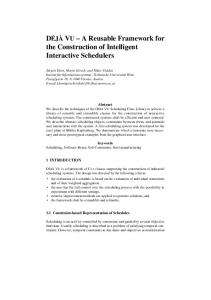
problem using genetic algorithms, including how the encoding of the model will be accomplished [18] or how to formulate the problem in order to keep its parametric dimension low. All these, if not confronted appropriately, could result in poor performance or scalability constraints in the design of a model [19]. In the following sections we propose a computational model building framework based on genetic algorithms by optimizing different neural networks to perform various behaviors. Section II outlines the model building framework focusing on how the neural networks of the model are configured based on the tasks they participate. Section III describes how the framework can automate the process of constructing a computational model of parieto-frontal and premotor regions to grasping. Section IV discusses implications of the model building framework in the context of computational modeling. The paper is concluded in section VI. II. MODELING FRAMEWORK Our model building framework employs genetic algorithms as an optimization tool, to fine tune a group of biologically inspired neural networks. The construction of the model is carried out in 9 steps based on the specifications provided by the user, at three levels, (i) neural, (ii) neural network and (iii) system. The steps that progress from the user specification of the biological model to the construction of the computational model are shown in fig 1. At initiation (step 1) the user inputs the number of brain regions that the computational model will include, the types of neuron models that will be used to encapsulate the regions and the allowed connectivity among those regions. This allows the framework to generate the initial structures of CRNs (see section IIA), as populations of neurons arranged in network layers (step 2).

during step 2, the framework assigns component roles (see section IIA) to each neuron in the Neural Networks and generates a net of interconnected CRNs. (step 4). The correlation parameters that the user provides (step 5) along with the tasks that were defined during step 3 are used to create the task association tree (see section IIC) (step 6) upon which the task genetic populations are based (step 7). The chromosomes encoding the populations generated during step 7 are used to evolve the networks produced during step 4 (step 8), and construct the final model (step 9). In the following section we describe how the framework accomplishes all of these steps, by focusing on issues regarding the modeling of each brain region, the encoding of the model and the definition of the task descriptors and association tree. A. Computational Region Network In our framework, each brain region is modelled using a distinct neural network, referred to as Computational Region Network (CRN). Each CRN is composed of three components: (i) clusters of interconnected neurons, (ii) input layers and (iii) sole neurons. All three components use the neuron model described in section III. Clusters contain groups of neurons that can be either inhibitory or excitatory, depending on the type of their connections. Excitatory clusters ensure that the appropriate levels of excitation will be maintained across neurons within a CRN, while inhibitory ones prevent the saturation (i.e. constant firing) of individual neurons. Sole neurons do not belong to a specific cluster, and can be either excitatory or inhibitory. The input layers within a CRN accept neuron signals from other networks and propagate it towards clusters and sole neurons within the CRN (fig 2). Different CRNs are densely connected by forming connections from the components of one population towards the components of another. Within a CRN, connections are sparsely formed between (i) different sole neurons (ii) clusters towards sole neurons and (iii) input layers towards clusters and sole neurons. The weights of these connections are updated according to the correlation based rule of Spike Time Dependent Synaptic Plasticity (STDP) [20]. STDP, as opposed to traditional Hebbian synaptic plasticity rules, ensures that correlated input activity between neurons will give rise to increased variability in the post-synaptic responses [21] and that non-casual relationships between neurons will not be enforced [22].

Fig 1. The model building steps that are carried out by our framework. The first column shows the user specifications, the second column shows the structures that are generated by the framework, while the third column shows the outputs produced by the framework.

Using the task descriptors (see section IIC) that are defined by the user (step 3) and the data structures generated

Fig 2. A Computational Region Network (square group of neurons) used for modelling a brain region in the biological model. It consists of excitatory (top left neuron group), inhibitory (bottom right), input (right column and top row) and sole (marked in black) neurons.

The structure of a CRN has been purposely subdivided into three components in order to promote the assessment of the dynamics and emergent properties in the final working model (see later the Discussion section). These components are not evaluated equally by the genetic algorithm. The fitness functions that describe a specific response property for the neurons of a CRN are evaluated using the sole neuron group. In contrast, the fitness functions that describe a general property for the area, e.g. average activation, are assessed at both the clusters of neurons and the sole neurons. B. Model Encoding The partitioning of a neural network to three distinct component types (clusters, inputs and sole neurons) helps at reducing the size of the encoding string for each CRN drastically. In addition it allows the encoding of the network to be more detailed for components that are required to encapsulate biological properties (sole neurons), and less thorough for components that are used to regulate processes within the CRN (clusters of neurons). The explicit definition of a distinct binary string for each CRN component helps at exploiting the closely correlated non-linear interactions within a CRN without interruptions during crossover operations [18]. Each neuron is encoded using three different parameters, the threshold value (θ), the resistor capacitance (R) and the membrane potential time constant (τ m ). All these are described in eqs (1-3) of section III. Within each cluster, all neurons are treated uniformly. Therefore for the encoding of the cluster components, our modeling framework, instead of including explicitly each neuron’s properties in the chromosome string, encodes the parameters of a Gaussian distribution (mean and standard deviation), for each physiological parameter of the cluster (θ, R, τ m ). This distribution is then used to sample values for each of the properties of the neurons in the cluster (fig 3).

Fig 3. The decoding from the cluster chromosome string to a Gaussian distribution, which in turn is used to sample different initialization properties for each neuron in the cluster. The chromosome string (left) is used to encode three different Gaussian distributions for each of the physiological parameters of the neurons in the cluster. These distributions are then used to initialize all neurons within the cluster.

Due to this cluster encoding scheme only three parameters are encoded for each ensemble of neurons. This helps to reduce the size of the encoding string from 3*n (3 parameters for the n neurons in the cluster) to a constant number. An additional bit is used to encode the excitation status of a cluster (excitatory or inhibitory). The sole neuron components of a CRN are used to encapsulate the functional properties of a brain region we

wish to model in more detail within the CRN (e.g. region exhibiting selectivity on a particular stimulus, or correlate different neuronal firings). For this reason each of the three physiological parameters of a sole neuron is encoded explicitly (i.e. using a separate string) within the chromosome representation. Input layers of a CRN are used to establish connections between different regions. Recent studies have shown that suppressing the Neural Network inputs in intermediate layers can help towards identifying potential representations that exist in the inputs. To ensure that the diversity of these representations will be appropriately depicted in the input neurons’ firings of the CRN, our model encodes all three neuron parameters within the chromosome string, as in the case of sole neurons. In addition to the physiological parameters of the neurons our modeling framework also encodes prospectus connectivity among components of CRNs. Two types of inter-connectivity (i.e. connections between different CRNs) and three types of intra-connectivity (connections within the same CRN) are allowed. The permitted connections that are formed between different CRNs are created among (i) clusters towards sole neurons and (ii) sole neurons towards sole neurons. To ensure that the resulting model will be biologically consistent, each CRN contains a vector of the regions it is allowed to connect to. Among components of the same CRN connections are formed between (i) input layers to sole neurons and clusters (ii) clusters towards sole neurons and (iii) sole neurons towards sole neurons. Each prospectus connection is encoded by the algorithm as (i) the percent of neurons that are to be connected among the different components (ii) the degree of excitation (i.e. percent of excitatory connections) that is to be created and (iii) an additional bit that describes whether a connection will be formed between the two components. In the case of the input components of the CRN the framework also includes the weight of each connection in the encoding of the chromosome string. This enables genetic evolution to exploit in greater detail the transmission between CRNs, and ensures that the appropriate representations that exist in the inputs will be communicated appropriately. C. Task Encoding Our framework builds and configures the networks of the computational model by optimizing their performance on different combination of tasks. Tasks define the desired behavior that should be exhibited by one or a combination of CRNs. A task can range from the execution of a behavior by the whole computational model to enforcing neurons within a CRN to acquire a specific firing pattern. The definition of a task includes the CRNs that it will use, the components (inputs, sole or clusters) of these CRNs that are allowed to be evolved, whether additions of new components (neurons or clusters) are allowed by the algorithm as well as the functional descriptions of the task (i.e. a function describing the desired behavior for each of these components).

the algorithm in order to select those individuals that performed satisfyingly on the task. These sampled chromosomes are used as initialization parameters for the individuals of the next task population in queue. III. COMPUTATIONAL MODEL OF GRASP RELATED REGIONS In the following section we outline the details of a grasp model that involves parieto-frontal and premotor regions (IT, V6a, AIP, F2, F5). Furthermore we show how the construction of this model can be automated by our framework.

Fig 4. The assignment of different tasks on every CRN component of a computational model. In this example tasks 3 and 4 are concerned with specific neuron groups of the same CRN. Only the second task involves the connectivity of all regions in the model, while the remaining ones include only a subset of the CRNs (gray circled networks). Tasks are defined by specifying the neurons that will be evolved, the CRN that includes those neurons and its underlying connectivity, the CRN components that belong to the task network and any additional constraints that should be considered by the algorithm.

Each task is assigned its own population of chromosomes and is evolved individually from others. This allows the parallelization of the model building framework, a very important property when it comes to computationally intensive operations. At the initialization of the framework each task population (i.e. population of chromosomes that are used to evolve the networks of the model in order to perform a specific task) defines the components of the CRNs that it will evolve and if required, integrates additional clusters or sole neurons to the networks (fig 4). Because of this formulation, the framework is able to identify the neurons of a CRN that are included in every task, and evolve them independently of other non-related neurons. As a result new tasks can be added on demand without affecting the already evolved components of the network. Tasks are associated with other tasks according to a correlation parameter. This parameter indicates the degree of involvement of neurons from other tasks in the current population of chromosomes. The framework uses this parameter in order to decide the percent of inbound connections from other tasks that will be attempted by the algorithm during evolution. All these are wrapped in an association tree (see the example in fig 7), which defines the order of evolution of the tasks during the construction of the model, and the extent to which a task can employ the already evolved neuronal structure of a different task for its own purposes. Tasks that are independent from others are placed in the top of the tree, and are evolved in the initial stages. Tasks that are highly correlated to others (i.e. they depend on inbound connections from other tasks) are evolved in the final stages of the evolutionary procedure. After the evolution of each task, a resampling operation takes place by

A. Biological Inspiration Recent neurobiological experiments in Macaques have revealed that there are visual and motion responsive neurons distributed in several parieto-frontal regions that are involved in the execution of grasp movements. In a recent study [23] the Anterior Intraparietal area (AIP) has been found to have 77% of visually responsive neurons, that were activated during an object fixation task. These neurons exhibited selectivity to the features of the objects that were presented. This selectivity is attributed to the connections of AIP with the inferotemporal cortex [24] in the ventral stream, which encodes the intrinsic object properties (i) concavity and convexity of an object [25] (ii) shape (20% of the neurons) and color (6% of the neurons) [26]. Moreover, neurons in the anterior Intraparietal were classified into three types (i) visuo-motor neurons (ii) visual dominant neurons and (iii) motor neurons. Visual dominant neurons link towards area F5 and are attributed the visual affordances that are employed by the motor system. Region F2 has been found to have a somatotopic organization (i.e. specific neuron clusters are assigned to specific body parts) with approximately 16% of its neurons being visually responsive. In addition it has been identified as a low excitable region with large percent of neurons being responsive to pro-prioception and tactile stimulus [27]. The distal forelimb field of the F2 contains 3 classes of neurons (i) purely motor (ii) visually modulated and (iii) visuo-motor neurons [28]. The purely motor class has been found to be selective for the type of prehension that was executed at any moment. The second class was modulated by the visual feedback of the object being grasped while the visuo-motor class discharged during both object fixation and grasping execution. Area F2 receives connections from region V6A [29], which encodes among other properties stimulus orientation, and narrowly from AIP [30].

Fig 5. The connectivity of the corresponding regions included in our model.

The ventral pre-motor area F5 of the premotor cortex plays an important role in the control of grasping [31]. It contains neurons that are correlated to specific goal-related distal motor acts. In addition, F5 contains another class of neurons selective to the presentation of objects. In general the AIP-F5 circuit is attributed the visuomotor transformation for grasping. In the following section we describe the specifications that are provided to our model building framework in order to construct the model shown in fig 5, focusing on issues such as neuron models, input encoding, task definition, experiment setup and the definition of neuronal functional roles. B. Neuron Models To reproduce the cortical functions of the primate brain, it is important to take into consideration the (i) distributiveness of the brain structures and the (ii) non-linearity of the response of the computational units. In our simulations we have adopted the standard form of the formal Leaky Integrate and Fire (LIF) neuron model [32]. The internal dynamics of each neuron are described by a differential equation (1) that models the fluctuations of the membrane potential variable (u) due to the driving current (I) passing through the neuron: 𝜏𝜏𝑚𝑚

𝜕𝜕𝜕𝜕 = −𝑢𝑢(𝑡𝑡) + 𝑅𝑅𝑅𝑅(𝑡𝑡) (1) 𝜕𝜕𝜕𝜕

where R and τ m are the resistor and membrane potential time constants. In LIF models, spikes are characterized by their firing time 𝑡𝑡 (𝑓𝑓) , which is the moment that the potential crosses a threshold value (θ): 𝑡𝑡

(𝑓𝑓)

: 𝑢𝑢�𝑡𝑡

(𝑓𝑓)

� = 𝜗𝜗 𝑎𝑎𝑎𝑎𝑎𝑎

𝑑𝑑𝑑𝑑(𝑡𝑡) � > 0 (2) 𝑑𝑑𝑑𝑑 𝑡𝑡 = 𝑡𝑡(𝑓𝑓)

After the emission of a spike, the membrane potential is reset to a constant value 𝑢𝑢𝑟𝑟 < 𝜗𝜗. lim

𝑡𝑡→𝑡𝑡(𝑓𝑓);𝑡𝑡>𝑡𝑡(𝑓𝑓)

𝑢𝑢(𝑡𝑡) = 𝑢𝑢𝑟𝑟 (3)

Equations 1, 2, 3 describe the model used for the neurons in the cluster, sole and input components of a CRN. A second population is used for modelling neurons that are selective to specific values of a parameter. These neurons are initialized to respond maximally to a specific value of an environment variable (the tuning value), and reduce the spike emissions proportionally to its permutations. The membrane potential fluctuations for this second class of neurons are described by eq. 4. (𝑎𝑎−𝑘𝑘)2 𝜎𝜎

𝑝𝑝 = 𝑝𝑝𝑟𝑟 ∗ 𝑒𝑒 −0.5∗

(4)

The membrane potential (p) of these tuning neurons is set to an exponential function of the tuning value k. The width of the tuning curve is set by the tuning sigma variable (σ). Spike emission occurs when the membrane potential of the neuron, exceeds the threshold value (p r ). The actual variable that the neuron encodes is set in the (a) parameter. The encoded variable is then described in the model using a population of neurons tuned to different values (using variations of the a parameter). A population of these tuning neurons was used for encoding different environment and object properties of the model into neural code. C. Computational model of the parieto-frontal and premotor regions to grasping Based on the data discussed in section IIIA we have used our framework to construct a computational model of the parieto-frontal and premotor regions (IT, V6a, AIP, F2, F5) that are involved in grasping by focusing on the specific visual, motor and visuo-motor dominant neurons that exist in these regions (fig 5). For our experiments we have used the Webots simulation platform, a commercial physics simulator that includes a realistic embodiment of the Hoap2 robot. Input encoding For our experiments we employ three different objects (sphere, box, and ring) with distinctive contours (fig 6). All of these objects have been shown to stimulate the visual responsive neurons in regions F5 and AIP and initiate different grasp behaviors through the AIP-F5 circuit (see section IIIA).

Fig. 6: The depiction of the three objects used in the model. From left: Ring, box and sphere.

These objects are processed using the MATLAB simulation software, to calculate various intrinsic properties ((i) convexity (ii) concavity (iii) perimeter (iv) orientation (v) holes) that are used as object identifiers in our computational model. To identify the edges of each object we use the derivative of a Gaussian filter to detect local maxima in the gradients of its image [33]. Table 1: List of the intrinsic object properties for each object

Perimeter Edges Corners Convexity Concavity Orientation Holes

Ring 1.2 0 0 0.5 0.1 0 1

Box 1.5 8 6 0.9 0.5 10 0

Sphere 1.3 0 0 0.2 0.2 5 0

To detect the corners of the objects we employ the HarrisStephens operator [34]. The results are illustrated in table 1.

The CRN encapsulating area IT is used to encode the properties of holes, perimeter, edges and corners using the tuning neuron class described in section IIIB. Two different classes of neurons were pre-coded, each having a tuning curve that was selective to a specific range for each of these properties. The CRN used for area V6a was used to encode the parameters of convexity and concavity.

descriptor is summarized on Table 2. The properties of each task descriptor are summarized on section IIC.

CRN Task group

F5, AIP, F2 IT, V6a, AIP, F2, F5

Task functional descriptions Our model encodes two types of functions, at a neural and a system level. At the neural level we model the selectivity exhibited by various neuron classes in three different regions of the model (F2, F5, AIP) for different types of properties, according to eq. 5.

Additions Constraints Fitness Task index

No None Eq. 6 1

𝑓𝑓𝑠𝑠𝑠𝑠𝑠𝑠𝑠𝑠𝑠𝑠𝑠𝑠𝑠𝑠𝑠𝑠𝑠𝑠𝑠𝑠𝑠𝑠 (𝑥𝑥) = � �3 − � 𝑁𝑁

∑𝑛𝑛=1..3 𝑖𝑖𝑛𝑛 �� (5) 𝑖𝑖𝑚𝑚𝑚𝑚𝑚𝑚

Equation 5 calculates an index of the selectivity of a neuron in a CRN, for a particular property, i.e. measures the extent to which the cell discharge of a neuron (i n ) deviates in relation to the maximum (i max ). In practice, we have used the selectivity index (proposed in [35] to resolve the direction tuning of particular neurons) with k=3, i.e. our three objects. Therefore the function provides a quantitative measure of the degree to which neurons in a region are tuned to a particular object (ring, sphere or box). At a system level the model is evaluated based on its ability to initiate and execute correctly the appropriate type of grasp, based on the object it is presented. To evaluate this function we assess the extent to which the appropriate fingers of the agent (according to the correct type of grasp on each trial) make contact with the object. This is shown in the following equation. 𝑓𝑓𝑔𝑔𝑔𝑔𝑔𝑔𝑔𝑔𝑔𝑔 = � 𝑡𝑡𝑐𝑐 (6) 𝑇𝑇

where 𝑡𝑡𝑐𝑐 are the sensor values of the fingers of the robot that are required to be used in order to form the grasp type that is executed during each cycle. T is the overall time of an execution trial. As a result, eq. 6 outputs values proportional to the time that the robot grasped the object using the appropriate fingers. Task Definition In order to translate the biological system description of section IIIA to a set of task descriptors we need to identify the evolving neurons that will be associated with each task, correlations among different tasks and whether additions of new components (clusters or sole neurons) will be allowed for a specific task. At the system level, the model is evolved to perform three different grasp behaviors, according to the object it is presented during each cycle. Each grasp is evaluated using eq. 6 to determine where the correct fingers of the agent made contact with the object. This system level task

Table 2. Task descriptor for the execution of grasp. Execution of appropriate grasp

For the Anterior Intraparietal region we defined three different types of tasks, each involving the configuration of of the four classes of neurons it contains (Table 3). Since neuron classes in this region are selective to either visual or prehension types we have also included the CRNs modeling the IT in the task network. Table 3. The task descriptors for region AIP. Three tasks are shown involving configuring the visuo-motor, visual dominant and motor neuron classes that exist in the region. Visuo-Motor

Visual Dominant

Motor

CRN

AIP

AIP

AIP

Task group Additions Constraints

V6a, IT Yes None

V6a, IT Yes None

V6a, IT Yes None

Fitness Task index

Eq. 5 2

Eq. 5 3

Eq. 5 4

For region F2, we defined three supplementary tasks in order to encapsulate the response properties of the neurons that exist in the region. In addition we have included a constraint for the CRN to enforce low-excitable threshold potentials in its neurons (using a decrease in the fitness of each chromosome, proportional to the thresholds of the neurons). The final descriptors for the tasks involved in this region are shown in Table 4. Table 4. Task descriptors for region F2. Three tasks were defined for each of the corresponding neurons classes of the visual and motor responsive neurons that exist in the region. VisuoMotor

Visual Dominant

Motor

CRN Task group

F2 IT, V6a, AIP

F2 IT, V6a, AIP

F2 IT, V6a, AIP

Additions

Yes

Constraints

Low-excitable threshold

Fitness Task index

Eq. 5 5

Yes Low-excitable threshold Eq. 5 6

Yes Low-excitable threshold Eq. 5 7

Finally in our computational equivalent of region F5 we have modeled two classes of neurons. The first class was selective to specific types of grasps, while the second class of neurons involved the selectivity on object presentation. Table 5 summarizes the task descriptors for the region.

Table 5. Task descriptors for region F5. Two tasks were defined for each of the corresponding neurons classes of the visual and grasp responsive neurons that exist in the region.

CRN Task group Additions Constraints Fitness Task index

Grasp selectivity

Object selectivity

F5 IT, V6a, AIP, F2 Yes None Eq. 5 8

F5 IT, V6a, AIP, F2 Yes None Eq. 5 9

Task associations The final step of the descriptions passed in our framework involved the definition of the correlations among different tasks. Since neurons in the F5 region encode directly the selectivity to object features from the visual processing regions (IT, V6a) the tasks involved in configuring those visually selective neurons were highly correlated (using a parameter of 30%) to the visually selective neuron tasks of regions F2 and AIP. This helped the algorithm to seek with a higher probability inter-connectivity patterns when configuring the F5 region in the AIP and F2 visual responsive neurons, where neuron selectivity was more transparent. Tasks that refer to the same CRN were correlated using a parameter of 10% (in order to promote connections among different component types of the same CRN). Finally the grasp system task was correlated to all region tasks using a correlation parameter of 20%. The final task association tree is shown in fig. 7.

Fig. 7. The task association tree for the three regions in our computational model. Tasks are marked with an ID number, which is their index in tables 2-5. In the graph correlated tasks are connected with an arrow, and marked with their correlation parameter.

D. Results We used 9 different populations of chromosomes, one for each of the 9 tasks that were described in the previous section. When each evolutionary procedure exceeded a threshold of 90% fitness, the framework proceeded to the next population of chromosomes, by sampling 80% of the evolved individuals. At the final model, all networks acquired the desired classes of neurons. The CRN encapsulating the F5 region acquired both classes of neurons described in section IIIA (30% of the sole neurons were selective to the grasp types and 20% of the sole neurons

were selective to the object vision). The F2 CRN acquired all three classes of neurons. Visual-dominant neurons required 20% of the whole population, motor neurons 30% of the population and visuo-motor neurons an approximate 10% of the population. Finally neurons in the AIP CRN acquired all three classes, with 20% of the neurons being visually modulated, 10% of the neurons motor modulated and 30% visuo-motor neurons. IV. DISCUSSION A. Computational Region Network The architecture of a CRN was designed to promote the consistency between the simulated and biological data according to the level of abstraction chosen for the model. For this reason, CRNs were structured from three components, clusters (neuronal ensembles), input layers and sole neurons. The clusters had three important roles: (i) to capture the broad-spectrum dynamics of the elements of the biological organism that are not modeled directly in the computational system, (ii) to regulate the average firing rates of the network and, (iii) to prevent saturation of the sole neurons. The last two roles are the result of the common excitation status that has been imposed to clusters. For the first role, consider for example the structural organization of the primary motor cortex. It consists of a large number of neurons that respond in different ways depending on different stimuli. To model accurately this region one should include a proper model for each neuron that exists in the primary motor cortex of the Macaque, and even then the modeling would be insufficient to explain accurately the functional role of the region [36]. The structure of a CRN, which corresponds to a functional module in the biological system, confronts this complexity by including clusters of homogeneous neurons (e.g. possessing the same physiological and excitation properties) which are modulated in common strategies (e.g. a change in excitation applies to all neurons in the cluster) by the genetic algorithm. Since the latter optimizes the model by grounding its functional modules on a behavior the response of the clusters will be altered appropriately to fit the task at hand. Thus, clusters at the optimal population are bound to capture at a certain extent different elements of the region’s functional roles, since they are also modified by the GA to suite the response of the biological equivalent area. The role of the sole neurons of the network is to encapsulate the specific operating role we wish to assign to a CRN. This inherent subdivision helps to study the dynamics of the model more thoroughly since there is an obvious separation in the elements of a CRN to the ones that fit a specific functional role (sole neurons), neuron ensembles (clusters) and the region’s input (input layers). B. Model building framework Due to their loose requirements in specifications, GAs can act as a sufficient framework for automating the construction of computational modes. In such framework, networks

representing different brain regions can be built out of functional specifications of the systems they wish to describe. The validity and detail of a model in this case is dependent on the assumptions and justifications the researcher makes for the biological system. According to Webb [4] this often becomes a problem of appropriately describing a system based on the constraints imposed by the environmental characteristics. This poses an additional problem of describing the terrain and embodiment characteristics in addition to the biological observations. Even though our framework does not include any real-world specifications of how these features can be accurately described in the framework of the model, the task specification framework can integrate these features incrementally, using appropriate tasks for each feature. V. CONCLUSION We have illustrated how with the use of GAs computational models of biological systems can be constructed, and applied the technique on a model of parieto-frontal and premotor regions for grasping. In the future we plan to extend our framework to include descriptions of the constraints and specifications commonly found in natural systems, directly in the evolutionary operators. In addition we plan to test the framework in different natural systems, and introduce mechanisms for evaluation directly in the GA.

[15]

[16]

[17]

[18]

[19]

[20]

[21]

[22]

[23]

[24]

[25]

REFERENCES [1]

[2]

[3]

[4] [5] [6]

[7] [8] [9]

[10]

[11] [12]

[13] [14]

M. Mojarrad, and M. Shahinpoor, “Biomimetic robotic propulsion using olmeric artificial muscles,” Proceedings of the IEEE international conference on Robotics and Automation, pp. 2152-2157, 1997. E. Hourdakis, H. E. Savaki, and P. Trahanias, “Computational modeling of cortical pathways involved in action execution and action observation,” Artificial Life, Submitted. R. S. Fearing, K. H. Chiang, M. Disckenson et al., “Wing transmission for a micromechanical flying insect,” Proceedings of the IEEE international conference on Robotics and Automation, pp. 15091516, 2000. B. Webb, “What does robotics offer animal behaviour?,” Animal Behaviour, vol. 60, pp. 545-558, 2000. A. H. Fagg, and M. A. Arbib, “A model of primate visual-motor conditional learning,” Adaptive Behaviour, vol. 1, pp. 1-37, 1992. A. Billard, “Learning motor skills by imitation: A biologically inspired robotic model,” Cybernetics and Systems, vol. 32, no. 1, pp. 155-193, 2001. I. Segev, “Single neuron models: Oversimple, complex and reduced,” Trends in Neurosciences, vol. 15, pp. 414-421, 1992. C. Koch, Biophysics of computation: Oxford University Press, 1999. M. A. Arbib, "Schema theory," The Encyclopedia of Artificial Intelligence, 2nd Edition, S. Shapiro, ed., pp. 1427-1443: WIleyInterscience, 1992. L. P. Kaelbling, and S. J. Rosenschein, “Action planning in embedded agents,” Robotics and autonomous systems, vol. 6, no. 1-2, pp. 35-48, 1990. R. D. Beer, Intelligence as adaptive behaviour, San Diego, CA USA: Academic Press Professional Inc., 1990. A. Cangelosi, S. Nolfi, and D. Parisi, “Cell division and migration in a genotype for neural networks,” Network Computation in Neural Systems, vol. 5, pp. 497-515, 1994. S. Nolfi, and D. Parisi, "Growing Neural Networks," The Handbook of Brain Theory and Neural Networks, M. A. Arbib, ed., 1991. M. Maniadakis, E. Hourdakis, and P. Trahanias, “Modeling

[26]

[27]

[28]

[29]

[30]

[31]

[32] [33]

[34] [35]

[36]

overlaping execution/observation pathways,” Proceedings of the International joint conference of artificial neural networks, 2007. H. E. Savaki, V. Raos, and M. N. Evangeliou, “Observation of action: grasping with the mind's hand,” Neuroimage, vol. 23, no. 1, pp. 193201, 2004. T. P. Caudell, and C. P. Dolan, "Parametric connectivity: Training of constrained networks using genetic algorithms," Proc. of the third international conference on genetic algorithms and their applications, J. D. Schaffer, ed., San Mateo: Morgan Kaufmann, 1989. X. Yao, “A review of evolutionary artificial neural networks,” International Journal of Intelligent Systems, vol. 8, no. 4, pp. 539-567, 1993. R. K. Belew, J. McInerney, and N. N. Schraudolph, Evolving Networks: using genetic algorithm with connectionist learning, Computer Science & Engineering Department (C-014). University of California, San Diego, La Jolla, 1991. H. Kitano, “Designing neural networks using genetic algorithms with graph generation system,” Complex Systems, vol. 4, pp. 461-476, 1990. S. Song, K. D. Miller, and L. F. Abbott, “Competitive Hebbian learning through spike-timing-dependent synaptic plasticity,” Nature Neuroscience, vol. 3, no. 9, pp. 919-926, 2000. C. F. Stevens, and A. M. Zador, “Input synchrony and the irregular firing of cortical neurons,” Nature Neuroscience, vol. 1, no. 3, pp. 210-217, 1998. T. J. Sejnowski, “Storing covariance with nonlinearly interacting neurons,” Journal of Mathematical Biology, vol. 4, no. 4, pp. 303-321, 1977. A. Murata, V. Gallese, G. Luppino et al., “Selectivity for the Shape, Size, and Orientation of Objects for Grasping in Neurons of Monkey Parietal Area AIP,” Journal of Neurophysiology, vol. 83, no. 5, pp. 2580-2601, 2000. G. Luppino, A. Murata, A. Belmalih et al., “Ventral visual stream information to the AIP-F5 circuit for grasping: A tracing study in the macaque monkey,” in Society for Neuroscience Abstracts Program, 2004. P. Jansen, R. Vogels, and G. Orban, “Macaque inferior temporal neurons are selective for disparity-defined three dimensional shapes,” Proceedings of the National Academ of Science, vol. 96, pp. 82178222, 1999. R. Desimone, T. D. Albright, G. C. Charles et al., “Stimulus-selective properties of inferior temporal neurons in the macauqe,” The Journal of Neuroscience, vol. 4, no. 8, pp. 2051-2062, 1984. L. Fogassi, V. Raos, G. Franchi et al., “Visual responses in the dorsal premotor area F2 of the macaque monkey,” Experimental Brain Research, vol. 128, pp. 194-199, 1999. V. Raos, M. A. Umilta, V. Gallese et al., “Functional Properties of Grasping-Related Neurons in the Dorsal Premotor Area F2 of the Macaque Monkey,” Journal of Neurophysiology, vol. 92, no. 4, pp. 1990-2002, 2004. M. Matelli, P. Govoni, C. Galletti et al., “Superior area 6 afferents form the superior parietal lobule in the macaque monkey,” Journal of Computational Neurol, vol. 402, pp. 327-352, 1998. G. Luppino, A. Murata, P. Govoni et al., “Largely segregated parietofrontal connections linking rostral intraparietal cortex (areas AIP and VIP) and the ventral premotor cortex (areas F5 and F4),” Experimental Brain Research, vol. 128, pp. 181-187, 1999. M. Jeannerod, M. A. Arbib, G. Rizzolatti et al., “Grasping objects: The cortical mechanisms of visuomotor transformation,” Trends Neuroscience, vol. 18, pp. 314-312, 1995. R. B. Stein, “Some Models of Neuronal Variability,” Biophysical Journal, vol. 7, no. 1, pp. 37-68, 1967. J. Canny, “A computational approach to edge detection,” IEEE Transactions on Pattern Analysis and Machine Intelligence, vol. PAMI-8, no. 6, pp. 679-698, 1986. C. Harris, and M. Stephens, “A combined corner and edge detector,” Alvey Vision Conference, vol. 15, pp. 50, 1988. S. L. Moody, S. P. Wise, G. di Pellegrino et al., “A model that accounts for activity in primate frontal cortex during a delayed matching-to-sample task,” J Neurosci, vol. 18, no. 1, pp. 399-410, 1998. D. P. Maki, and M. Thompson, Mathematical Models and Applications, Englewood Cliffs: Prentice Hall, 1973.