file systems or database tablespaces). Data protection tech- niques exploit the workload's update properties to effec- tively make secondary copies of the data, ...
A Framework for Evaluating Storage System Dependability Kimberly Keeton and Arif Merchant Storage Systems Department HP Labs, Palo Alto, CA 94304 kimberly.keeton,arif.merchant�@hp.com Abstract—Designing storage systems to provide business continuity in the face of failures requires the use of various data protection techniques, such as backup, remote mirroring, point-in-time copies and vaulting, often in concert. Predicting the dependability provided by such compositions of techniques is difficult, yet necessary for dependable system design. We present a framework for evaluating the dependability of data storage systems, including both individual data protection techniques and their compositions. Our models estimate storage system recovery time, data loss, normal mode system utilization and operational costs under a variety of failure scenarios. We demonstrate the effectiveness of these modeling techniques through a case study using real-world storage system designs and workloads. 1 Introduction Data is the primary asset of most corporations in the information age, and businesses must be able to access that data to continue operation. In a 2001 survey, a quarter of the respondents estimated their outage costs as more than $250,000 per hour, and 8% estimated them as more than $1M per hour [5]. The price of data loss is even higher– bankruptcy, in the limit. Dependable data storage systems are needed to avoid such problems. Fortunately, many techniques exist for protecting data, including tape backup [3], mirroring and parity-based RAID schemes for disk arrays [20], wide area inter-array mirroring [12], snapshots [1] and wide area erasure-coding schemes [15]. Each technique protects against a subset of the possible failure scenarios, and techniques are often used in combination to provide greater coverage. Unfortunately, the multitude of data protection techniques, coupled with all of their configuration parameters, often means that it is difficult to employ each technique appropriately. System administrators often use ad hoc techniques for designing their data storage systems, focusing more on setting configuration parameters (e.g., backup windows), rather than on trying to achieve a particular dependability [3, 4]. As a result, it is often unclear whether the business’ dependability goals have been met. If we could quantify the dependability of a storage system, we could evaluate whether an existing storage system meets its dependability goals, explore future designs and what-if scenarios (to allow users to understand the dependability ramifications of their design choices), and pro-
vide the inner-most loop of an automated optimization loop to choose the “best” solution for a given set of business requirements [13]. Such a framework should permit the composition of data protection techniques, to model complicated storage systems and facilitate the incorporation of new techniques as they are invented. This paper describes a modeling framework for quantitatively evaluating the dependability of storage system designs. By dependability, we mean both data reliability (i.e., the absence of data loss or corruption) and data availability (i.e., that access is always possible when it’s desired). Because our target is tools for use in the business continuity community, we have consciously adopted their metrics for recovery time and recent data loss after a failure. Recovery time measures the elapsed time after a failure before a business service (e.g., application) is up and running again; the recovery time objective (RTO) provides an acceptable upper bound [2]. When a failure occurs, it may be necessary to revert back to a consistent point prior to the failure, which will entail the loss of any data written after that point. Recent data loss measures the amount of recent updates (expressed in time) lost during recovery from a failure; the recovery point objective (RPO) provides an upper bound [2]. Both RTO and RPO may range from zero to days. Following the common practice of the business continuity community, our models evaluate the recovery time and recent data loss metrics under a specified failure scenario. To these metrics, we add normal mode system utilization and overall system cost (including capital and service cost outlays and penalties for violating business requirements). The primary contributions of our work include: 1) a common set of parameters to describe the most popular data protection techniques; 2) models for the dependability of individual data protection techniques using these parameters; 3) techniques for composing these models to determine the dependability of the overall storage system; and 4) analysis of the models and compositional framework using case studies. The remainder of the paper is organized as follows. Section 2 provides an overview of popular data protection techniques and surveys related work. Section 3 describes our modeling framework in detail, and Section 4 provides an extensive case study drawn from real-world storage designs to demonstrate its operation. Finally, Section 5 concludes.
2 Data protection techniques and related work Disk arrays are typically used to store the primary copy of data; they provide protection against internal hardware failure through RAID techniques [20] and redundant hardware paths to the data. Other failures, such as user or software errors and site failure, are covered by techniques that periodically make secondary copies of the data, often to other hardware. These secondary copies preferably reflect a consistent version of the primary copy at some instant in time; we call these versions retrieval points, or RPs. The main classes of such techniques are mirroring, point-in-time copies and backup. Mirroring keeps a separate, isolated copy of the current data on another disk array, which may be co-located with the primary array or remote. Mirrors may be synchronous, where each update to the primary is also applied to the secondary before write completion, or asynchronous, where updates are propagated in the background. Batched asynchronous mirrors [12, 21] coalesce overwrites and send batches to the secondary to be applied atomically; they lower the peak bandwidth needed between the copies by reducing the volume of updates propagated and smoothing out update bursts. A point-in-time (PiT) image [1] is a consistent version of the data at a single point in time, typically on the same array. The PiT image may be formed as a split mirror, where a normal mirror is maintained on the same array until a “split” operation, which stops further updates to the mirror, or as a virtual snapshot, where a virtual copy is maintained using copy-on-write techniques, with unmodified data sharing the same physical storage as the primary copy. Most enterpriseclass disk arrays (e.g., [6, 9]) provide support for one or more of these techniques. Backup is the process of copying RPs to separate hardware, which could be another disk array, a tape library or an optical storage device. Backups may be full, where the entire RP is copied; cumulative incremental, where all changes since the last full backup are copied; or differential incremental, where only the portions changed since the last full or incremental are copied. Tape backup is typically done using some combination of these alternatives (e.g., weekend full backups, followed by a cumulative incremental every weekday). Backups made to physically removable media, such as tape or optical disks, can also be periodically moved to an off-site vault for archival storage. Backup techniques and tools have been studied from an operational perspective (e.g., [3, 4]). Studies also describe alternative mechanisms for archival and backup (e.g., [15]) and filesystems that incorporate snapshots (e.g., [11]). Evaluations of the storage system dependability have focused mainly on disk arrays, including the dependability of array hardware and RAID mechanisms and the recovery time after failure (e.g., [7, 17, 18, 19, 20, 22]). Additionally, a great deal of work (e.g., [8]) focuses on the overall area of dependability and performability evaluation of computer
systems. Keeton, et al., have explored issues in automating data dependability [13]. This paper builds upon and complements these techniques by providing models of individual dependability techniques and a framework for composing them, thus enabling the evaluation of dependability in storage systems that combine multiple dependability techniques. Our models are deliberately simple, in order to allow users to reason about them, and are designed to be composable, so as to fit in the overall framework. 3 Modeling storage system dependability The goal of our modeling framework is to evaluate the dependability of a storage system design for the specified workload inputs and business requirements, under the specified failure scenario. Table 1 summarizes the model’s parameters, which are explained in the sections below. The model components work together as follows. The data protection technique models convert their input parameters to bandwidth and capacity workload demands on the storage and interconnect devices they employ. The hardware device models perform device-specific calculations to determine each device’s bandwidth and capacity utilization and outlay costs. The compositional models combine the results from these data protection and device models to generate the output metrics. By isolating the details of each data protection technique and hardware device, we can easily substitute more sophisticated models (e.g., [16, 19]) for these components as needed, without needing to modify the rest of the modeling framework. In this section, we describe the modeling framework in more detail, including: how we capture the model inputs (Section 3.1); how we abstract the behavior of individual data protection techniques (Section 3.2); and how we compose techniques to determine the dependability of the overall storage design (Section 3.3). 3.1 Model inputs This section outlines how we describe model inputs, including workloads, business requirements and failure scenarios. 3.1.1 Workload inputs A storage system holds the primary copy for data (e.g., file systems or database tablespaces). Data protection techniques exploit the workload’s update properties to effectively make secondary copies of the data, with some techniques propagating all updates and others propagating only periodic batches of unique updates. Given these behaviors, the key workload parameters to capture include: data capacity, average access rate, average update rate, burstiness and batch update rate, as defined in Table 1. Although most systems store multiple data objects, we assume for simplicity a single data object and workload. Our models can be extended in a straightforward manner by explicitly tracking each object’s workload demands, the set
Parameter Notation Output metrics system utilization recovery time recent data loss overall cost Model inputs: workload data capacity dataCap average access rate avgAccessR average update rate avgUpdateR burstiness burstM batch update rate batchUpdR(win) Model inputs: Business requirements data unavailability penalty rate unavailPenRate recent data loss penalty rate lossPenRate Model inputs: Failure scenarios and recovery goals failure scope failScope
Units
Description
percentage sec sec US dollars
utilization of maximally utilized storage component time from failure to having application running again recent data updates not recovered by recovery process overall system cost (including outlays and penalties)
bytes bytes/sec bytes/sec multiplier bytes/sec
size of the data item rate of read and write accesses to the object rate of (non-unique) updates to the object ratio of peak update rate to average update rate unique update rate within a given window
US dollars/sec US dollars/sec
penalty per unit time for unavailability of data penalty for loss of a time-unit’s worth of updates to data
����� ����� � � ��� � ��
set of data copy sites unavailable due to a failure
recovery time target recTargetTime sec Model inputs: Storage system design—data protection techniques accumulation window accW sec propagation window propW sec hold window holdW sec cycle count cycleCnt count cycle period cyclePer sec retention count retCnt count retention window retW sec copy representation copyRep �� ���� � propagation representation propRep �� ���� � Model inputs: Storage system design—device configuration maximum capacity slots maxCapSlots count maximum bandwidth slots maxBWSlots count slot capacity slotCap bytes slot bandwidth slotBW bytes/sec enclosure bandwidth enclBW bytes/sec delay devDelay sec fixed costs fixCost US dollars capacity-dependent costs capCost US dollars/byte bandwidth-dependent costs bwCost US dollars/byte/sec spare type spareType
� ���� �����
spare provisioning time spareTime sec spare discount factor spareDisc multiplier
point in time to which restoration is requested period over which updates are batched to create a retrieval point (RP) RP transmission period delay between receiving and transmitting an RP number of secondary windows between primary windows length of a cycle for a policy with multiple accumulation windows number of cycles of RPs simultaneously retained how long a particular RP is retained what RP representation is maintained what RP representation is propagated max slots for capacity devices (tape cartridges, disks) max slots for bandwidth devices (tape drives, disks) per-slot (tape cartridge or disk) capacity per-slot (tape drive or disk) bandwidth aggregate enclosure bandwidth (including busses and controllers) delay for accessing storage device/interconnect propagation delay fixed costs for enclosure, facilities, service per-capacity costs for device, facilities, service per-bandwidth costs for device, facilities, service spare resources available for device time to provision spare resources fraction of original dedicated resource cost
Table 1: Summary of parameters used in dependability modeling framework.
of techniques and underlying storage devices used to protect the object, and inter-object dependencies during recovery. 3.1.2 Business requirement inputs The business consequences of data unavailability and data loss are assessed through two business inputs: data unavailability penalty rate and recent loss data penalty rate [13], as defined in Table 1. These penalty rates will be used, in conjunction with the recovery time and recent data loss output metrics, to calculate the penalties incurred under the imposed failure scenario. The penalties and outlays comprise the overall cost of the storage system. 3.1.3 Failure scenario inputs Our models evaluate the recovery time and recent data loss metrics under a specified primary copy failure scenario, rather than capturing the effects of different failures,
weighted by their frequency. Given that the law requires companies to plan for infrequent failures, and that such events may result in bankruptcy, in practice most disastertolerant systems are designed to meet a hypothesized disaster, regardless of its frequency. The failure scope, which describes the set of failed storage and interconnection devices, represents the failure scenario to be considered. The scope may be one of several pre-specified, named sets, such as: disk array, building (all the devices in the building), site (all devices on the site), and geographic region (all the devices in the region). Additionally, the failure scope data object indicates loss or corruption of the object (due to user or software error) without hardware failures. The recovery time target is the point in time to which restoration is requested. Under most circumstances, the recovery target time is “now” – the time just before the failure.
Shared spare site Primary building/site Host
Host
Primary Storage-area network array level 0: Disk array primary Tape lib copy level 2: tape level 1: backup split mirror
Secondary site level 3: Tape vault remote vaulting Tape lib
Remote mirror (opt)
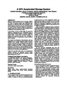
Figure 1: Example storage system design. This design provides the basis for the running example in Section 3.
However, in case of a data loss due to user error or a software virus, the recovery target would be before the error. 3.2 Modeling data protection techniques We model the primary and secondary copies as a hierarchy, where each level in the hierarchy corresponds to either the primary copy or a technique used to maintain secondary copies. Each level is responsible for retaining some number of discrete retrieval points (RPs), and for propagating RPs to the next level in the hierarchy. We adopt the convention that the primary data copy is level 0. As the level numbers increase, the data protection techniques typically store less frequent RPs, possess larger retention capacity, and exhibit longer recovery latencies. Figure 1 illustrates an example storage system design. The hierarchy used to represent the design is as follows: in addition to the primary copy (level 0), the primary array also stores split mirrors (level 1), which are used to perform backup (level 2) to a local tape library. Finally, tapes are periodically shipped offsite to a remote vault (level 3). We will describe the policy and configuration parameters for these levels in more detail in Section 3.2.1. The storage system design should also express a recovery path, which describes the levels that will help to restore the primary copy under the imposed failure scenario. By default, the recovery path may be merely the reverse of the RP propagation hierarchy. As an optimization, some levels may be skipped if they would only contribute additional recovery latency (e.g., PiT copies for site disaster recovery). The source of the recovery path must be a level in the RP propagation hierarchy. 3.2.1 Data protection technique configuration parameters The key insight behind our models is that data protection techniques share a central property: their basic operations are the creation, retention and propagation of RPs. We exploit this property to choose a single set of parameters to abstract their operation. This consistent representation can then be used to compose the data protection techniques. Differences between techniques (and between different configurations of the same technique) are expressed through these configuration parameters.
In general, the data protection technique at level i receives RPs from level i 1� and retains the last retention count ( �����i ) RPs. The RPs may be maintained as full or partial copies, as specified by the copy representation (���� �� i ). Each RP is stored for a retention window ( �� i ) (related to �����i ). Every accumulation window (��� i ) hours, a new RP is propagated to level i. It is held for the hold window ( � � i ) before being transferred during the propagation window (� �� i ), using a full or partial propagation representation (� �� ��i ). Finally, some techniques use a cycle with multiple propagation representations: for example, tape backup may use a full propagation every weekend followed by a cumulative incremental every weekday. The number of secondary windows in the cycle is denoted ��� ����i and the cycle length (time) is ��� ��� i . Separate accumulation, propagation and hold windows may be specified for each of the secondary propagation representations. Figure 2 illustrates these key parameters for the example system shown in Figure 1. We adopt several conventions about the relationship between parameters. First, to maintain the flow of data between the levels, � �� should be no longer than ��� . Second, because lower levels of the hierarchy generally represent larger, slower (or more distant) storage media, we assume that they may retain more, and more infrequent, RPs; hence ����� � ����� and ��� � ��� ��� . Thus, the range of time represented by the RPs at slower levels of the hierarchy will be at least as long as the range at faster levels, due to the longer accumulation windows and/or larger retention counts used at the slower levels. Third, � � should generally be no longer than �� , to avoid placing additional retention capacity demands for devices involved in providing level i. �
�
�
3.2.2 Device configuration parameters A storage system dependability model also requires knowledge of the physical storage and interconnect devices and their configurations. Each storage device is represented by an operational model, which computes the device’s normal mode bandwidth and capacity utilizations, and a cost model, which computes the outlay costs, broken down by data protection technique. We abstract the structure and operation of hardware devices into the parameters described in Table 1. All storage devices have enclosures, bandwidth components (e.g., disks and tape drives) and capacity components (e.g., disks and tape cartridges). Bandwidth components have a maximum bandwidth value (� ��� ), and capacity components have a maximum capacity value (� �����). Enclosures provide physical limitations on the number of bandwidth components (���� � ���), the number of capacity components (������� ���), and the aggregate device bandwidth (��� � ). Device costs are calculated using fixed (������), capacity-dependent (�������) and bandwidthdependent (������) cost components. Devices may also have an access delay (����� ��) (e.g., tape load and seek
0: primary copy
1: split mirror
time
RP1 RP2 RP3 RP4 RP5 RP6 RP7 RP
now
time
0: primary copy
accW1=12hr; holdW1=0; propW1=0
RP1 RP2 RP3 RP4 RP5 RP6 RP RP
1: split mirror
RP RP RP RP
holdW2=1hr accW2=1wk
2: tape backup
3: remote vaulting
propW2=48hr
retCnt1=4; retW1=2 days
RP1
2: tape backup
holdW3=4wk + 12hr accumW3=4wk
RP
RP retCnt2=4; retW2=4 wk
RP1
propW3=24hr
3: remote vaulting
RP retCnt3=39; retW3=3 years
Figure 2: Parameter specification for example in Figure 1. Split mirrors are generated every twelve hours, and propagated immediately, with a negligible hold window. Each split mirror is retained for two days, resulting in a retention count of four. Data is backed up once a week to the tape library. For ease of exposition, we choose a simple backup policy that creates only full backups, using a one-week window to accumulate updates, followed by a one-hour offset and a 48-hour propagation (e.g., backup) window. For example, backup propagation might begin at midnight on Saturday, and end at midnight on Monday. The tape library retains each backup for four weeks. As the backup retention window expires every four weeks, the oldest tapes are shipped offsite to the remote vault via the mid-day overnight shipment, resulting in a hold window of four weeks + twelve hours and a propagation window of 24 hours. The vault retains each RP for three years.
time, interconnect propagation time). Similarly, the model for interconnect devices characterizes their bandwidth, delay and costs. We include physical transportation methods, such as courier services, under interconnect devices. Additionally, each storage and interconnect device may have a specified spare (��� �����) that should replace it if it fails. Each spare resource has its own device characteristics, plus a provisioning time (��� �����) that determines how quickly it can be used, and a cost computed using a discount factor (��� �����). Provisioning times may be short for dedicated hot spares, but more substantial for shared resources. The cost of the shared resource may be correspondingly lower — a fraction of the full cost. 3.2.3 Data protection technique workload demands For each hardware device model to evaluate its normal mode utilization, it must know what demands are being placed on it. As a result, the data protection technique models convert their input parameters to a set of bandwidth and capacity workload demands on the storage and interconnect devices involved in each level. Here we qualitatively describe these workload demands; we refer the interested reader to a technical report [14] for more details. We model an update-in-place variant of virtual snapshot PiT copies, which assumes that old values are copied to a new location before an update is performed, resulting in an additional read and write for every foreground workload write. Snapshots require sufficient additional capacity to store the unique updates accumulated during ��� . Our split mirror PiT copy model assumes that a circular buffer of split mirrors is maintained, with the least recently used mirror always undergoing resilvering (being brought up-to-date). Our convention is that ����� mirrors are ac-
cessible, and an additional split mirror is maintained to facilitate resilvering, for a total of ����� � 1 mirrors. When a mirror becomes eligible for resilvering, the system must propagate all unique updates that have occurred since that mirror was last split ����� � 1 accumulation windows ago. This requires reading the new value from the primary copy and writing it out to the mirror. Synchronous, asynchronous and asynchronous batch inter-array mirroring place bandwidth demands on the interconnect links and the destination array and capacity demands (equal to the data capacity) on the destination array. Interconnect bandwidth demands vary between the different mirroring protocols based on their operation, as described in Section 2. Because many arrays support alternate interfaces for inter-array mirroring, we assume that no additional bandwidth requirements are placed on the source array’s client interface. For the asynchronous variants, we do not explicitly model the buffer space used to smooth write bursts and coalesce updates, as it is typically a small fraction of the typical array cache. Backup reads data from the source array and writes it to the destination backup device. The required bandwidth for each device is the maximum bandwidth required for the full backup (to transfer the entire dataset during the full � �� ) and for the largest cumulative incremental backup (to transfer all updates incurred since the last full backup during the incremental � �� ). Our backup model places no capacity demands itself on the source array, making the assumption that another technique (e.g., split mirror or virtual snapshot) will be employed to provide a consistent copy of the data. Capacity demands for the backup device include ����� cycles’ worth of data, plus an additional full dataset copy.
Each cycle includes one full backup plus ��� ���� cumulative incrementals, where each incremental is larger than the last. The additional full dataset copy avoids problems from failures that occur while a new full backup is being performed. Finally, remote vaulting places no additional bandwidth or capacity demands on the tape backup device, provided � ��
. In the case that � � that � � ��
, the backup device must make an additional copy of the tapes, so that they may be shipped offsite before the end of the retention window. We assume that only full backups are sent offsite to be retained at the vault. �����
�� ��
3.3 Composing data protection techniques In this section, we describe how we compose the data protection techniques to calculate the overall model output metrics, including normal-mode system utilization, recent data loss, recovery time and overall system costs. 3.3.1 Normal mode utilization The normal mode utilization model verifies that the underlying device configuration can support the RP creation and propagation workloads described by the policies in the storage system design. The calculation is performed in two steps: first, each hardware device model computes its own (local) utilization, and then a separate (global) calculation determines the overall system utilization. This decomposition allows details of the internal device architecture to be localized in the device models. Once all workload demands have been enumerated, each hardware device model evaluates whether the sum of the demands on that device can be satisfied by its capabilities. More formally, the model for each hardware device d calculates the following: numTech ������ � ∑i�1 ��� � � ������� numTech ����� � ∑i�1 �� � � �����
Here numTech is the number of data protection techniques; ������ is the maximum capacity for device d, computed as ������� ��� � � �����; ���� is device d’s maximum bandwidth, computed as max ��� � � ���� � ��� � � ��� �. The global model determines the overall system utilization (e.g., ������ and ����� ) as that of the most heavily utilized device and generates an error if ������ � 1 or ����� � 1.
3.3.2 Retrieval point propagation
time
(retCnt-1)*cyclePer i+1: post-receipt of new RP (retCnt-1)*cyclePer
(now – (holdW+propW))
i+1: pre-receipt of new RP (now – (holdW+propW+accW))
�����
�� ��
now
i+1: guaranteed range
(now – ((retCnt-1)*cyclePer+ holdW+propW))
(now – (holdW+propW+accW))
Figure 3: Range of RPs guaranteed to be present at a level.
A level’s time lag relative to the primary copy varies, depending on when the most recent RP arrived, as shown in Figure 3. Just after an RP arrives, the level is out-of-date by � � � � �� , the hold window plus the propagation window. Just before the next RP arrives, the level is outof-date by as much as � � � � �� � ��� . (For the j multi-level case, these values generalize to ∑i�1 � � � j � �� � and ∑i�1 � � � � �� � � ��� for level j, respectively.) The retention period for the level is ����� 1� � ��� ��� . Our goal is to calculate the worst-case recovery time and recent data loss, so we want to determine the range of time that is guaranteed to be present at the level. As a result, we can only consider the overlapping portions of these regions: � ��� ����� 1� � ��� ��� � � � � � �� ����� ��� � � � � �� � ��� ���, as shown in the figure. Generalizing to the case of multiple composed levels, the guaranteed range of time at level j ����� 1� � ��� ��� � ∑i�1 � � � j is: � ��� j � �� ������ ��� ∑i�1 � � � � �� � � ��� ��. �
�
�
�
�
�
3.3.3 Recent data loss We want to determine which level of the recovery hierarchy has the closest match for the recovery target in the range of RPs it currently maintains. Three cases are of interest for a level j. First, if the recovery target is too recent, an RP hasn’t yet propagated to this level. In this case, the recent data loss is merely the time lag of the level, as calculated in the previous section: ��� � � � � � �� . Generalizing to the composed case, the worst case recent data loss j for a level j is ∑i�1 � � � � �� � � ��� . Second, if an RP for the recovery target has propagated to this level, new RPs are arriving periodically every ��� time units. In this scenario, the worst case recent data loss is merely ��� . Third, if an RP for the recovery target is too old to be retained, the level cannot serve as the source for the recovery, and the worst case data loss is the entire data object. The level with the closest match serves as the data source for the recovery operation, with recovery time calculated as described in the next section. �
Determining the data loss and recovery time for an imposed failure scenario requires understanding at what level we can find an RP that closely matches the recovery time target. To do so, we must understand what time range is reflected at each level. This range can be calculated by considering how long it takes each RP to propagate to a given level (alternately, how “out-of-date” the level is, relative to the primary copy), as well as how much data is retained at that level.
�
�
failure
3.3.5 Overall system costs
recovered
time parFix: reprovision
0: primary copy
serFix: load+seek
1: tape backup 2: remote vaulting
serXfer: transfer F
serXfer: transfer I serFix: load+seek
parFix: ship tapes
Figure 4: Recovery time dependencies. An example recovery path for a primary array failure includes retrieving tape cartridges from a remote vault, reading them at the site’s tape library, and restoring their contents onto the primary array. Tape shipment from the vault must proceed before the tapes can be loaded at the local site’s tape library. Data transfer to the primary array cannot begin, however, until array resources have been adequately reprovisioned (a potentially long-latency operation). Recovery completes once the full backup and incremental backups (if any) are transferred.
3.3.4 Recovery time To estimate the worst-case recovery time for the imposed failure scenario, we consider both the tasks that must be performed at each level and whether those tasks can be overlapped with tasks at other levels. Figure 4 illustrates these components for an example recovery path. We abstract the recovery time computation using the following components. The parallelizable fixed period (�� ���) includes preparatory tasks before data arrives from another level, including device reprovisioning and reconfiguration, and negotiation for access to shared resources. The serialized fixed period (�� ���) includes tasks that can be started only after data arrives, such as tape load and seek times. The serialized per-byte period (�� � � ) includes data transfer operations, which may begin only when both the sender and receiver are ready. The transfer rate is limited to the minimum of the sender and receiver available bandwidth (e.g., the remaining bandwidth after any RP propagation workload demands have been satisfied). The recovery time can be computed recursively by determining the time at which each level is ready to serve as a source for the data. Intuitively, a level is ready to serve as a source for the data once it has received the transmission from the last level (after suitable parallelizable preparation on the parts of both levels), and followed by any additional serialized fixed preparation it must perform once the data arrives. The recovery time for a given level i, � , is computed as follows: � � max � � �� ��� � � �� � � � �� ��� � max � � �� ��� � � ����!�� min ���� � ����
� � �� ��� where ����!� is the amount of data to be recovered and ���� is the available bandwidth for the device. The overall recovery time is that of the primary copy ( e.g., � ). �
�
�
� �
�
�
Our cost model includes both outlays and penalties. Outlays cover expenditures for direct and indirect costs such as equipment, facilities, service contracts, salaries, spare resources and even insurance. Penalties are incurred when goals for data outage or recent data loss are violated. Outlays are calculated per data protection technique by each hardware device model. As with the utilization calculation, this decomposition allows the details of device internals to be localized inside the hardware device models. Most device-specific capital expenditures have fixed, percapacity and per-bandwidth components. Fixed costs may include disk array or tape library enclosures, service costs, fixed facilities (e.g., floorspace purchase or rental, cooling) costs, etc. Per-capacity components may include disks and tape media, floorspace-dependent costs, and variable cooling, power and service costs. Per-bandwidth components include disks, tape drives, and interconnect links. We assume that each device has a primary data protection technique, and potentially one or more secondary techniques (e.g., a disk array may store both the primary copy and split mirrors). We assume that the fixed costs, plus the relevant per-capacity and per-bandwidth costs are allocated to the primary data protection technique. Only the additional per-capacity and per-bandwidth costs associated with a secondary technique are allocated to that secondary technique. Spare resource costs are allocated to data protection techniques in a similar fashion. Penalties are calculated at a global level using the output values from the data loss and recovery time sub-models. The recent data loss penalty is calculated by multiplying the worst case data loss amount by the data loss penalty rate input parameter. Likewise, the data outage penalty is calculated by multiplying the worst case recovery time by the data outage penalty rate input parameter. 4 Case study In this section, we present a case study to illustrate the framework’s operation and validate its ability to compose models. We begin by examining a baseline configuration in detail, and then explore several what-if scenarios to improve the storage system’s dependability and cost. The case study demonstrates that the quantitative results produced are reasonable, and that the framework is flexible and useful in designing a system that meets dependability requirements. Our baseline configuration (Figure 1) employs split mirroring, tape backup and remote vaulting to protect the primary copy of the dataset. We model a workgroup server, whose measured workload characteristics are quantified in Table 2. Tables 3 and 4 summarize the policy and device configuration parameters for the data protection techniques used. Table 4 also presents models for calculating outlay costs. These models include fixed costs, per-capacity (c, in GB) costs, per-bandwidth (b, in MB/s) costs and pershipment (s) costs. The values for each term are calculated based on annualized hardware component costs (assuming a
dataCap 1360 GB
avgAccessR 1028 KB/s
avgUpdateR 799 KB/s
burstM 10X
batchUpdR(win) 1 min: 727 KB/s; 12 hr: 350 KB/s; 24 hr, 48 hr, 1 wk: 317 KB/s
Table 2: Parameters for cello workgroup file server workload used in case studies [12]. Technique Split mirror Tape backup Remote vaulting
accW 12 hr 1 wk 4 wk
propW 0 hr 48 hr 24 hr
holdW 0 hr 1 hr 4 wk + 12 hr
cyclePer 12 hr 1 wk 4 wk
retCnt 4 4 39
retW 2 days 4 wks 3 yrs
copyRep full full full
propRep full full full
Table 3: Data protection technique parameters for baseline storage system design.
Device Disk array Tape library
maxCapSlots @ slotCap (GB) 256@73GB 500@400GB
maxBWSlots @ slotBW (MB/s) 256@25MB/s 16@60MB/s
enclBW (MB/s) 512MB/s 240MB/s
devDelay (hr) n/a 0.01hr
Vault Air shipment
5000@400GB n/a
n/a n/a
n/a n/a
n/a 24hr
Costs 123297 � c � 17 2 98895 � c � 0 4 �b � 108 6 25000 � c � 0 4 s � 50
dedicated dedicated
spare Time (hours) 0.02hr 0.02hr
spare Disc 1X 1X
none none
n/a n/a
n/a n/a
spareType
Table 4: Device configuration parameters for baseline storage system design. The primary array is a mid-range array (based on HP’s EVA [9]) with up to 256 73-GB disks and up to 32 GB of cache. The tape library (based on HP’s ESL9595 [10]) contains up to 16 LTO tape drives and up to 500 LTO tape cartridges. These devices communicate through a Fibre-channel storage area network (SAN). Both the primary array and the tape library employ a dedicated hot spare. The primary site communicates via air shipment to a tape vault, which can contain up to 5000 tape cartridges; the vault uses no sparing.
three-year depreciation) and facilities costs. The component costs are based on actual list prices or expert estimates. The details of these component costs are omitted due to space limitations. We assume data unavailability and loss penalty rates of $50,000 per hour (each). We assume the use of hot spare resources at the primary site and a remote shared recovery facility. Hot spare resources take 60 seconds to provision, and cost the same as the original resources. Remote hosting facility resources can be provisioned (e.g., drained of other workloads and scrubbed) within nine hours. Because the resources are shared, they cost only 20% of the dedicated resources. We examine failures at three scopes: a data object, an array, and a site. The data object failure simulates a user mistake or software error that corrupts a 1 MB data object, requiring roll back to the version that existed 24 hours ago. The recovery hierarchy is simply the reverse of the RP propagation hierarchy. The array failure simulates failure of the primary array, and the site failure simulates a disaster at the primary site. Both require recovery of the entire dataset to its most recent state, and use a recovery hierarchy of the remote vault, tape backup, and primary copy. 4.1 Baseline configuration results Table 5 summarizes the bandwidth and capacity demands that the data protection techniques place on the underlying devices to manage RPs throughout the hierarchy. Primary disk array bandwidth is demanded by the foreground workload, split mirroring, and tape backup. Split mirror resilvering generates both read and write demands. The backup policy generates a read workload on the array and a write workload on the tape library. The vaulting pol-
Device Disk array Foreground workload Split mirror Backup Overall Tape library Backup Tape vault Vaulting
Bandwidth
Capacity
0.2% 0.6% 1.6% 2.4% (12.4 MB/s)
14.6% 72.8% 0.0% 87.4% (8.0 TB)
3.4% (8.1 MB/s)
3.4% (6.6 TB)
0.0%
2.6% (51.8 TB)
Table 5: Normal mode bandwidth and capacity utilization for baseline system.
icy’s accumulation window matches the backup retention window, meaning that the oldest full backup can be shipped offsite when its retention window expires and resulting in no additional tape library bandwidth demands. The total average bandwidth demands are 12.4 MB/s for the primary array and 8.1 MB/s for the tape library, resulting in an overall system bandwidth utilization of 4%. Each level’s retention window and copy representation type imposes capacity requirements on the underlying devices. The array stores both the primary copy and five split mirrors, each a full copy of the dataset, demanding 8.0 TB of total array capacity. The tape library maintains four full backups, corresponding to a total of 6.6 TB. Finally, the vault maintains 39 full backups, corresponding to 51.8 TB. The resulting overall system capacity utilization is 88%. Table 6 examines the dependability of the baseline storage system design for the three different failure scenarios. In the object failure case, the day-old target version is maintained at the split mirror level, and can be easily restored by an intra-array copy, resulting in a negligible recovery time.
Failure scope object array site
Recovery source split mirror tape backup remote vaulting
Recovery time 0.004 s 2.4 hr 26.4 hr
Recent data loss 12 hr 217 hr 1429 hr
Table 6: Worst case recovery time and recent data loss results for baseline system.
Overall costs (outlays + penalties)
$100,000,000
$71.9M
$11.9M $10,000,000
$1.6M $1,000,000
$100,000 object
array
site
Failure scope foreground wkld outlay vaulting outlay
split mirror outlay unavailability penalty
backup outlay loss penalty
Figure 5: Overall system cost for baseline system.
The worst case recent data loss is twelve hours, the cycle of split mirror RP creation. In the array failure case, both the primary copy of the dataset and the split mirror secondary copies are lost, requiring recovery from the local tape backup system. Data transfer from tape dominates the 2.4-hour array failure recovery time. Because the most recent updates haven’t yet propagated to the backup system, the worst case data loss is equivalent to the time lag of the backup level. Recovery from a site disaster must proceed from a copy stored at the remote vault. Securing access to hosting facility resources can proceed in parallel with the shipment of tapes from the remote vault. Once the new site has been provisioned and the tapes have arrived and been loaded, transfer of data can begin, resulting in a recovery time of 26.4 hours. The most recent updates haven’t yet been propagated to the vault, resulting in a sizable recent data loss. Figure 5 presents the overall costs for each failure scenario, including both the outlay costs for the data protection techniques, as well as the penalties that result from their recovery time and recent data loss. Penalty costs (in particular, recent data loss penalties) dominate for the array and site failures, due to the large lag times for the RPs present at the tape backup and vault. Outlay costs are split roughly evenly between the foreground workload, split mirroring and tape backup, with negligible contribution from remote vaulting. 4.2 What-if scenario results Table 7 presents results for several what-if scenarios intended to improve the baseline configuration’s dependability. Recovery from site disasters could be improved by modifying the remote vaulting policy. Shortening the accumulation window to a week would reduce the interval between
RPs, thus limiting the amount of recent data loss. Assuming that a retention window of the same duration is desired, this policy would increase the capacity demands at the vault. Table 7 shows that a weekly vaulting policy reduces site disaster data loss and associated penalties. Adding daily cumulative incrementals to the weekly full backups and weekly vaulting policy provides no benefit for site disasters, but decreases the recent data loss and penalty costs for array failures. This savings comes at the cost of slightly increased recovery time, due to the need to restore both a full backup and and incremental backup in the worst case. If, instead, a backup policy of daily full backups (with no incrementals) is used, array failure recovery time and data loss decrease. Site disaster data loss also decreases, due to the shorter propagation window used for the daily full backups, which implies a shorter vault time lag. A further, albeit modest, outlay cost savings can be achieved if virtual snapshots are used instead of split mirrors. Further recent data loss reductions are possible with asynchronous batch mirroring, which uses shorter accumulation and hold windows. Worst case recent data loss decreases dramatically to only two minutes. If a single wide-area link is used, transfer time dominates the recovery time. Recovery time can be reduced dramatically if more links are used. Site disaster recovery time is still greater than array failure recovery time, however, because of the longer delay to provision spare resources at the shared recovery site. Ironically, the lowest total cost comes from the single-link mirroring system, even though it has a higher data unavailability penalty, because the outlays are considerably lower. 5 Conclusions We have presented a framework for modeling storage system dependability. Following common practices from the business continuity community, this framework quantifies post-failure recovery time and recent data loss, as well as normal mode utilization and overall system costs. We have identified a single set of abstractions for modeling the dependability of the wide range of data protection techniques used today, including backup, remote mirroring, PiT copies and vaulting. These abstractions will facilitate the inclusion of new techniques as they become available. We have also shown how to compose these individual technique models into a model of the overall storage system’s dependability, permitting evaluation of storage system designs that combine these techniques. As shown by the case study, the models facilitate comparison of storage system designs, permitting storage administrators to make decisions based on their dependability business requirements, rather than on guesses as to whether their needs will be met. In the future, we plan to expand on this work in several ways. First, we plan to experiment with increasing levels of sophistication in the modeling framework components, including the workload description and hardware device and data protection technique models. Second, we plan to validate these models using measurements of recovery behav-
Storage system design Baseline Weekly vault Weekly vault, F+I Weekly vault, daily F Weekly vault, daily F, snapshot AsyncB mirror, 1 link AsyncB mirror, 10 links
Outlays $0.97M $0.99M $0.99M $1.01M $0.76M
RT (hr) 2.4 2.4 4.0 2.4 2.4
$0.93M $5.03M
21.7 2.8
Array failure DL (hr) Penalties 217 $10.97M 217 $10.97M 73 $3.85M 37 $1.97M 37 $1.97M 0.03 0.03
$1.09M $0.14M
Total cost $11.94M $11.96M $4.84M $2.98M $2.73M
RT (hr) 26.4 26.4 26.4 26.4 26.4
$2.01M $5.18M
21.7 9.8
Site disaster DL (hr) Penalties 1429 $70.97M 253 $13.97M 253 $13.97M 217 $12.17M 217 $12.17M 0.03 0.03
$1.09M $0.49M
Total cost $71.94M $14.96M $14.96M $13.18M $12.93M $2.01M $5.52M
Table 7: Recovery time (RT), recent data loss (DL) and cost results for what-if scenarios. Weekly vault indicates a weekly ��� and 12-hr �����. F+I represents weekly fulls and daily cumulative incrementals, with a 48-hr ��� and ����� for fulls, a 24-hr ��� and 12-hr ����� for incrementals, and a � �� � of 5. Daily F indicates 24-hr ��� and 12-hr ����� for fulls, with no incrementals. Snapshot indicates the use of virtual snapshots instead of split mirrors. AsyncB mirror indicates the use of asynchronous batch mirroring with 1-min ��� over 155 Mbps OC-3 links, with a cost model of b � 23535 (where b is in MB/s). If not explicitly specified, policy parameters are the same as in the baseline configuration.
ior from real-world systems. Third, we want to extend the model to handle an increased number of failure scopes and to evaluate degraded mode operation (e.g., under the failure of a data protection technique). Finally, we plan to incorporate this modular modeling approach into our ongoing work in automatically designing dependable storage systems [13]. The optimization framework in our automated tool allows us to incorporate failure frequencies and prioritizations, thus permitting the concurrent consideration of multiple failures in the design of dependable storage systems. Acknowledgements The authors are grateful to John Wilkes, Jeff Chase and Eric Anderson for their inputs on the direction of this work and comments on earlier versions of this paper. References [1] A. Azagury, M. E. Factor, and J. Satran. Point-in-Time copy: Yesterday, today and tomorrow. In Proc. IEEE/NASA Conf. Mass Storage Systems (MSS), pp. 259–270, Apr. 2002. [2] C. Brooks et al. Disaster recovery strategies with Tivoli storage management. IBM International Technical Support Organization, version 2 edition, Nov. 2002. [3] A. Chervenak, V. Vellanki, and Z. Kurmas. Protecting file systems: A survey of backup techniques. In Proc. IEEE/NASA Conf. MSS, pp. 17 – 31, Mar. 1998. [4] J. daSilva and O. Gudmundsson. The Amanda network backup manager. In Proc. 7th USENIX LISA Conf., pp. 171– 182, Nov. 1993. [5] Eagle Rock Alliance Ltd. Online survey results: 2001 cost of downtime. http://contingencyplanningresearch.com/2001 Survey.pdf, Aug. 2001. [6] EMC Corporation. EMC TimeFinder product description guide, Dec. 1998. www.emc.com/products/product pdfs/pdg/timefinder pdg.pdf. [7] G. A. Gibson and D. A. Patterson. Designing disk arrays for high data reliability. Journal Parallel and Distributed Computing, 17(1–2):4–27, January/February 1993. [8] B. Haverkort et al., editors. Performability modeling: techniques and tools. Wiley and Sons, May 2001.
[9] Hewlett-Packard Company. HP StorageWorks Enterprise Virtual Array, Dec. 2003. h18006.www1.hp.com/products/storageworks/enterprise/. [10] Hewlett-Packard Company. HP StorageWorks Extended Tape Library Architecture, Dec. 2003. h18006.www1.hp.com/products/storageworks/tlarchitecture/. [11] D. Hitz, J. Lau, and M. Malcolm. File system design for an NFS file server appliance. In Proc. USENIX Winter 1994 Technical Conf., pp. 235–246, Jan. 1994. [12] M. Ji, A. Veitch, and J. Wilkes. Seneca: remote mirroring done write. In Proc. USENIX Technical Conf. (USENIX’03), pp. 253–268, June 2003. [13] K. Keeton et al. Designing for disasters. In Proc. 3rd Conf. File and Storage Technologies (FAST), Mar. 2004. [14] K. Keeton and A. Merchant. A framework for evaluating storage system dependability – extended version. Technical Report HPL-2004-53, Hewlett-Packard Labs, Mar. 2004. [15] J. Kubiatowicz et al. Oceanstore: An architecture for globalscale persistent storage. In Proc. ACM Conf. ASPLOS, pp. 190 – 201. ACM, Nov. 2000. [16] A. Kuratti and W. H. Sanders. Performance analysis of the RAID 5 disk array. In Proc. IPDS’95, pp. 236–245. IEEE, Apr. 1995. [17] M. Malhotra and K. S. Trivedi. Data integrity analysis of disk array systems with analytic modeling of coverage. Performance Evaluation, 22(1):111–133, 1995. [18] A. Merchant and P. S. Yu. An analytical model of reconstruction time in mirrored disks. Performance Evaluation, 20(1–3):115–29, May 1994. [19] R. R. Muntz and J. C. S. Lui. Performance analysis of disk arrays under failure. In Proc. 16th VLDB, pp. 162 – 173, Aug. 1990. [20] D. A. Patterson, G. Gibson, and R. H. Katz. A case for redundant arrays of inexpensive disks (RAID). In Proc. ACM SIGMOD Conf., pp. 109–116, June 1988. [21] R. H. Patterson et al. SnapMirror: file-system-based asynchronous mirroring for disaster recovery. In Proc. 1st Conf. File and Storage Technologies (FAST), pp. 117–129, Jan. 2002. [22] S. Savage and J. Wilkes. AFRAID—A Frequently Redundant Array of Independent Disks. In Proc. USENIX Winter 1996 Technical Conf., pp. 27–39, Jan. 1996.