A framework for quad/triangle subdivision surface ... - Semantic Scholar

Volume 0 (1981), Number 0 pp. 1–14

A framework for quad/triangle subdivision surface fitting: Application to mechanical objects Guillaume Lavoué and Florent Dupont and Atilla Baskurt LIRIS UMR 5205, 43 Boulevard du 11 Novembre 1918, 69622 Villeurbanne, France [glavoue,fdupont,abaskurt]@liris.cnrs.fr

Abstract In this paper we present a new framework for subdivision surface approximation of 3D models represented by polygonal meshes. Our approach, particularly suited for mechanical or CAD parts, produces a mixed quadrangletriangle control mesh, optimized in terms of face and vertex numbers while remaining independent of the connectivity of the input mesh. Our algorithm begins with a decomposition of the object into surface patches. Then the main idea is to approximate first the region boundaries and then the interior data. Thus, for each patch, a first step approximates the boundaries with subdivision curves (associated with control polygons) and creates an initial subdivision surface by linking the boundary control points with respect to the lines of curvature of the target surface. Then, a second step optimizes the initial subdivision surface by iteratively moving control points and enriching regions according to the error distribution. The final control mesh defining the whole model is then created assembling every local subdivision control meshes. This control polyhedron is much more compact than the original mesh and visually represents the same shape after several subdivision steps, hence it is particularly suitable for compression and visualization tasks. Experiments conducted on several mechanical models have proven the coherency and the efficiency of our algorithm, compared with existing methods. Categories and Subject Descriptors (according to ACM CCS): I.3.5 [Computer Graphics]: Curve, surface, solid, and object representations G.1.2 [Numerical Analysis]: Approximation of surfaces and contours

1. Introduction The context of this work is the Semantic-3D project (http://www.semantic-3d.net). The objective is the transmission of 3D mechanical models through low bandwidth channels in a visualization objective on various terminals. The 3D model database to handle comes from the car manufacturer Renault, and contains thousands of quite irregular polygonal meshes representing CAD parts. Thus an efficient compression tool is needed to reduce the amount of data carried by this 3D content, knowing that the original NURBS information is not available. Many efficient techniques have been developed for encoding polygonal meshes [TG98, GS98, IS01] but fundamentally, this representation remains very heavy in terms of amount of data (a large points set, on top of the connectivity have to be encoded). Moreover, lossy compression schemes like wavelet based ones [KSS00,VP04] produce artifacts, visually damaging for smooth mechanical objects. Other models exist to represent a 3D shape: NURBS surc The Eurographics Association and Blackwell Publishing 2006. Published by Blackwell

Publishing, 9600 Garsington Road, Oxford OX4 2DQ, UK and 350 Main Street, Malden, MA 02148, USA.

faces or subdivision surfaces. These models are much more compact. A subdivision surface is a smooth (or piecewise smooth) surface defined as the limit surface generated by an infinite number of refinement operations using a subdivision rule on an input coarse control mesh. Hence, it can model a smooth surface of arbitrary topology (contrary to a NURBS model which needs a parametric domain) while keeping a compact storage and a simple representation (a polygonal mesh). Moreover it can be easily displayed to any resolution, according to the terminal capacity for example. Subdivision surfaces are now widely used for 3D imaging and have been integrated to the MPEG4 standard [MPE02]. In this context, we present an algorithm for fitting a piecewise smooth subdivision surface to an input mesh aiming at optimizing control points number and connectivity of the subdivision control polyhedron. Our method, based on mesh decomposition, is particularly suited for mechanical surfaces or CAD parts; indeed in these cases the research of the optimality is quite relevant. This algorithm is beneficial in terms of compres-

G. Lavoué, F. Dupont and A. Baskurt / Subdivision surface fitting for mechanical objects

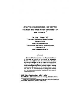
sion (the original mesh can be stored or transmitted in the form of a coarse control polyhedron), remeshing (the subdivided control polyhedron is often much more regular than the original mesh) or reverse engineering. Section 2 details the related work about subdivision surface fitting, while the overview of our method and the different choices that have been made are presented in section 3. Sections 4, 5, 6, 7 deal with the four distinct steps of our method: The decomposition of the object into surface patches, the approximation of their boundaries, the initialization and the optimization of the subdivision surfaces. Finally, in section 8, results are presented, evaluated and compared with existing methods. 2. Related Work Several methods already exist for subdivision surface fitting, most of them take as input a dense mesh, simplify it to obtain a base coarse control mesh and then displace the control points (geometry optimization) to fit the target surface. Lee et al. [LMH00], Ma et al. [MMTP04], Mongkolnam et al. [MRF03] and Marinov and Kobbelt [MK05] use the Quadric Error Metrics from Garland and Heckbert [GH97] for simplification. Kanai [Kan01] uses a similar decimation algorithm which directly minimizes the error between the original mesh and the subdivided simplified mesh. With these simplification based approaches, the control mesh connectivity strongly depends on the input mesh. For instance, figure 1 shows the approximation method from Kanai [Kan01] applied on two different meshes representing the same shape. It appears obvious that results are not the same. Particularly, the control polyhedron in Figure 1.e obtained for the bad tessellated mesh of Figure 1.d is not correct and gives a quite poor limit surface (see Figure 1.f) regarding to the original one. In our algorithm, in order to remain independent of the original connectivity, we first decompose the object into surface patches, and then we use the boundaries of the patches and the curvature information of the target object to transmit the topology to our control polyhedron. The fitting method from Suzuki et al. [Sus99] also remains independent of the target mesh connectivity, by iteratively subdividing and shrinking an initial hand defined control mesh toward the target surface. Unfortunately this method fails to capture local characteristics for complex target surfaces, and is only suited for genus 0 surfaces without holes. Jeong and Kim [JK02] use a similar shrink wrapping approach and encounter the same problems with complex topologies. In the same idea, Cheng et al. [CWQ∗ 04] construct an octree partition of the target surface and then triangulate it using the Marching Cube algorithm. Concerning the geometry optimization, Lee et al. [LMH00] and Hoppe et al. [HDD∗ 94] sample a set of points from the original mesh and minimize a quadratic error to the subdivision surface. This technique was recently improved by Marinov and Kobbelt [MK05] which introduce parameter corrections. Suzuki et al. [Sus99] propose a local and faster approach, also used in [JK02] and [MRF03]: The positions

of the control points are optimized, only by reducing the distance between their limit positions and the target surface. Hence only subsets of the surfaces are involved on the fitting procedure, thus results are not so precise. Litke et al. [LLS01] also introduce a local algorithm, based on quasiinterpolation, to compute detail coefficients on a CatmullClark surface. Ma et al. [MMTP04] consider the minimization of the distances from vertices of the subdivision surface after several refinements to the target mesh; our algorithm follows this framework while using not a point to point distance minimization, but a point to surface minimization, by considering the local quadratic approximants introduced by Pottmann and Leopoldseder [PL03]. This algorithm allows a more accurate and rapid convergence. The recent algorithms from Cheng et al. [CWQ∗ 04] and Marinov and Kobbelt [MK05] follow a similar way. To our knowledge, the optimality in terms of control point number and connectivity represents a minor issue in the existing algorithms but seems particularly relevant for mechanical or CAD objects. Only Hoppe et al. [HDD∗ 94] optimize the connectivity by trying to collapse, split, or swap each edge of the control polyhedron. Their algorithm produces high quality models but need of course an extensive computing time. Recently, Marinov and Kobbelt [MK05] subdivide faces associated with high errors and flip some edges to regularize vertex valences, similarly to Cheng et al. [CWQ∗ 04]. Our algorithm adapts the connectivity of the control mesh to the anisotropy of the target surface by analyzing its curvature directions, which reflect the natural parameterization of the object. The number of control points is also optimized by enriching iteratively the control polyhedron following different rules depending on the error distribution. Moreover this approach allows to directly control the approximation error, whereas simplification based methods [Kan01, MRF03, MMTP04, LMH00] indirectly control the error by modifying the decimation level.

Figure 1: Subdivision surface approximation for a simple object with the algorithm from Kanai et al. [Kan01].

c The Eurographics Association and Blackwell Publishing 2006.

G. Lavoué, F. Dupont and A. Baskurt / Subdivision surface fitting for mechanical objects

Figure 2: The different steps of our fitting scheme for the Fandisk object. (a) Segmentation, (b) boundaries extraction, (c) boundaries approximation, (d) subdivision control mesh, (e) limit surface. 3. Overview and orientation Our first objective is to obtain a base coarse control polyhedron with the same topology than the target mesh but independently of its connectivity and aiming at optimizing vertex and face numbers. Then, we wish to enrich and optimize this initial control polyhedron in terms of connectivity and geometry. Accordingly, our framework is the following (see Figure 2): • The target 3D object is segmented into surface patches (see Section 4), of which boundaries are extracted. The objective of this segmentation step is dual: Fitting a simple patch is easier than fitting a whole object, and the boundaries will help us to retrieve and transmit to the coarse base mesh, the topology of the target object. • The network of boundaries is approximated with piecewise smooth subdivision curves (defined by coarse control polygons)(see Section 5). This step provides a network of control polygons (see Figure 2.c), optimized in terms of control point number. • For each patch an initial approximating subdivision surface is created by linking the boundary control points (extracted from the network) with respect to the lines of curvature of the target patch (see Section 6). The corresponding control polyhedron connectivity is therefore adapted to the anisotropy of the target patch, with a quite low number of vertices and facets, since boundary control polygons are optimized. • The initial local control polyhedrons are enriched and optimized (connectivity and geometry) by iteratively moving control points and adding new ones according to the error distributions (see Section 7). The control mesh defining the whole surface is then created assembling every local control meshes. Our main contributions are the following: • The original global framework for subdivision surface fitting, based on segmentation and boundaries approximation. • The initialization algorithm, which creates a topologically correct approximating subdivision surface, independently of the connectivity of the target patch, and adapted to its anisotropy, while owning a near minimal vertex number. c The Eurographics Association and Blackwell Publishing 2006.

• The enrichment process which allows to directly control the approximation error, by adding iteratively new control points according to the error distribution, while optimizing the connectivity. The segmentation and the curve approximation algorithms are detailed in previous works, thus they are just briefly presented in this paper. The geometry optimization algorithm, which is a non trivial adaptation of the Pottmann and Leopoldseder’s Active B-Spline algorithm [PL03] to subdivision surfaces is also briefly presented since two recent subdivision surface fitting algorithms consider a similar approach [CWQ∗ 04] [MK05].

3.1. Curvature calculation Our whole fitting algorithm is, to a large extent, based on curvature tensors analysis, thus we have to calculate this information for the input 3D meshe. A triangle mesh is a piecewise linear surface, thus the calculation of its curvature is not trivial. We have implemented the work of Cohen-Steiner et al. [CSM03], based on the Normal Cycle. This estimation procedure relies on solid theoretical foundations and convergence properties and is quite robust even for bad tessellated objects. For each vertex, the curvature tensor is calculated and the principal curvature values kmin, kmax and directions dmin, dmax are extracted. They correspond respectively to the eigenvalues and eigenvectors of the curvature tensor, with switched order (the eigenvector associated with kmin is dmax and vice versa). The figure below presents samples of these fields for the Plane object. On the edges of the wings, we have a high maximum curvature, whereas kmin is null, it is a parabolic region. Kmin is positive on elliptic regions, like at the end of the wings, and negative in hyperbolic regions like at the joints between the wings and the body of the plane. The principal curvature directions have significance only on anisotropic regions (elliptic, parabolic and hyperbolic) where they represent lines of curvature of the object. On isotropic regions (spherical, planar), they do not carry any information.

G. Lavoué, F. Dupont and A. Baskurt / Subdivision surface fitting for mechanical objects

this scheme, although being C2 almost everywhere, remains only C1 at extraordinary points and around triangle/quad boundaries. Even if our mechanical surfaces are likely to be quadrics (this is often the case of CAD parts), this loss of quadratic precision is not a limitation because our objective is not a perfect fitting of the target objects but rather a correct approximation for a visualization purpose.

Figure 3: Curvature fields for the 3D object Plane. (a) Kmax, (b) Kmin (absolute value), (c) dmax, (d) dmin. 3.2. The choice of the subdivision scheme Within our approximation framework, we have to choose a subdivision scheme. Many subdivision rules exist, some of them are adapted for triangular control meshes, like Loop [Loo87] and others are adapted for quadrilateral ones, like Catmull-Clark [CC78]. For a given surface to approximate, the choice of the appropriate subdivision scheme is critical. Indeed, even if in theory any triangle can be cut into quads or any quad can be tessellated into triangles, results are not equivalent. The fact is that the nature of the control polyhedron (quads or triangles) strongly influences the shape and the parameterization of the resulting subdivision surface. The body of the cylinder, for instance, is much more naturally parameterized by quads than by triangles. These reasons have led us to chose the hybrid quad/triangle scheme developed by Stam and Loop [SL03]. This scheme reproduces Catmull-Clark on quad regions and Loop on triangle regions. At each subdivision step, the base mesh is firstly linearly subdivided: Each edge is split into two, each triangle into four and each quad into four (see Figure 4). Secondly, each vertex is replaced by a linear combination of itself and its direct neighbors. When a vertex is entirely surrounded by triangles or quads we use smoothing masks of Figure 5.a and Figure 4.b and otherwise we use the mask from Figure 5.c, which depends on the numbers of edges (ne ) and quads (nq ) surrounding the vertex. Concerning smoothness analysis, we have to notice that

Figure 4: Example of quad/triangle subdivision. (a) Control mesh, (b,c) one and two subdivision steps, (d) limit surface.

Figure 5: Smoothing masks for Loop (a), Catmull-Clark (b) and the quad-triangle scheme (c) (extracted from [SL03]). 4. Decomposition into patches The problem of subdivision surface fitting is quite complex to resolve, particularly in our case, since we aim at remaining independent of the target mesh connectivity. Hence we have chosen to previously segment the object into near constant curvature surface patches. Benefits are numerous: The inverse subdivision problem is simplified whereas boundaries of the patches can be used to retrieve the topology and simplify the fitting process. Moreover this decomposition may bring adaptivity for the visualization (we can imagine, once we have the complete control polyhedron, subdivide only a desired part of the object). We use the segmentation method described in [LDB05a]. This decomposition is based on the curvature tensor field analysis and presents two distinct complementary steps: A region based segmentation (see Figure 6.a) which decomposes the object into near constant curvature patches, and a boundary rectification based on curvature tensor directions, which corrects boundaries by suppressing their artifacts or discontinuities. This rectification step which is critical for our fitting algorithm is illustrated on figure 5. Even if the region segmentation (see Figure 6.a) shows good qualitative results in terms of general shape and disposition of the segmented regions, boundaries are often jagged and present artifacts; the rectification algorithm will analyze the coherency between curvature directions (see Figure 6.b) of the object and boundaries of the segmented regions to suppress incorrect boundary edges (see figure 6.c) and extend good ones (see figure 6.d). Resulting segmented patches, by virtue of their properties (constant curvature, clean boundaries) are thus particularly adapted to subdivision surface fitting. c The Eurographics Association and Blackwell Publishing 2006.

G. Lavoué, F. Dupont and A. Baskurt / Subdivision surface fitting for mechanical objects

Figure 7: Illustration of segmentation (a), boundary extraction (b) and subdivision curve approximation (c).

Figure 6: The different steps of the Boundary Rectification (algorithm from [LDB05a]) for the Fandisk object with a zoom on an artifact correction. (a) Region based segmentation. (b) Minimum curvature directions. (c) Correct boundary edges extraction and marking (incorrect ones are in red, others in green). (d) Final boundaries after extension. 5. Boundaries approximation Once the 3D object has been segmented, our algorithm approximates the network of patch boundaries with subdivision curves. At first, pieces of boundary are extracted; a piece of boundary is a polyline corresponding to the boundary between two distinct patches (see figure 7.b). Then, each piece of boundary is approximated with a subdivision curve, associated with a control polygon. Every control polygons are then assembled (junction points are tagged as sharp) (see figure 7.c) to give a control polygon network (see Figure 2.c). The purpose of this network is to simplify and optimize the further subdivision surface fitting algorithm. This approach bears some similarities with lofting algorithms, like that proposed by Schaefer et al. [SWZ04] which aims at building a subdivision surface over a network of curves. Then, considering a surface patch, its boundary control polygons can then be extracted from the network; according to subdivision properties, these control polygons will represent the boundaries of the control polyhedron of the approximating subdivision surface. 5.1. Subdivision curve presentation A subdivision curve is created using iterative subdivisions of a control polygon (see Figure 8). In this paper we use the subdivision rules defined for surfaces by Hoppe et al. [HDD∗ 94] for the particular case of sharp or boundary edges: New vertices are inserted at the midpoints of the conc The Eurographics Association and Blackwell Publishing 2006.

trol segments and new positions Pi0 for the control points Pi are computed using their old values and those of their two neighbors using the mask: 1 Pi0 = (Pi−1 + 6Pi + Pi+1 ) (1) 8 With these rules, the subdivision curve corresponds to a uniform cubic B-Spline, except for its end segments. We also consider specific rules (those defined by Hoppe [HDD∗ 94] for corner vertices) to handle sharp parts and extremities: Pi0 = Pi

(2)

This subdivision curve will coincide with the boundary generated by commonly used subdivision surface rules like Catmull-Clark [CC78], Loop [Loo87] or the quad-triangle scheme from Stam and Loop [SL03].

Figure 8: Example of subdivision curve with one sharp vertex. (a) Control polygon. (b,c) 2 iterations of subdivision. (d) Limit curve. 5.2. The approximation algorithm This curve fitting algorithm approximates efficiently a polygonal curve with a piecewise smooth subdivision curve, while minimizing the control points number. It is an extension for subdivision rules, including sharp vertex processing, of the Active B-Spline Curve developed by Pottmann and Leopoldseder [PL03]. This algorithm considers also a theoretical framework, analyzing curvature properties of subdivision curves, which computes a near optimal evaluation of

G. Lavoué, F. Dupont and A. Baskurt / Subdivision surface fitting for mechanical objects

the number and positions of the control points. Describing this curve approximation method is beyond the scope of this paper, thus we invite readers to refer to [LDB05b] for complete explanations and details about this algorithm. A result is illustrated on Figure 7.c. 6. Local subdivision surface initialization 6.1. Overview Once the control polygon network has been created, an initial subdivision surface is created for each patch. The purpose of the initialization process is dual: Transmit the topology from the target surface patch to the initial control polyhedron and optimize the connectivity of this control polyhedron regarding to the anisotropy of the target surface. The initialization algorithm is the following: First, for each patch, the corresponding control polygons representing its boundaries are extracted from the network, and then our process will attempt to connect control points from these control polygons (we call them boundary control points), in order to create the better set of facets that will represent the initial control polyhedron. These edges will be chosen according to the curvature directions of the target patch. According to these edges, the topology is then reconstructed in a simple and efficient manner. Boundary control polygons have to be synchronized, before launching the surface initialization process. Indeed, considering a cylinder, the curve approximation will produce two square-like control polygons for example, however since these boundaries are approximated independently, nothing guaranties than control polygons are aligned. Hence, we process a synchronization: Closed control polygons associated with constant curvature target curves (i.e circles) are aligned together. We rotate them so as to move their first control point closer to a fixed limit infinite position. 6.2. Edge score definition The purpose is to create edges and facets by connecting the boundary control points in such a way that the corresponding created initial subdivision surface is the better approximation of the target surface for these given control points, regarding to the resulting error. For this purpose, we consider the lines of curvature of the target surface, represented by local directions of minimum and maximum curvature (see Figure 9.b and c). We call Control lines of a subdivision surface, the smooth lines coming from the subdivision of the edges of the control polyhedron (see Figure 4.d and 9.a). These Control lines are strongly linked to the lines of curvature. Indeed the topology of a control polyhedron will strongly influence the geometry information of the associated limit surface, which is also carried by lines of curvature [ACSD∗ 03]. This coherency between control lines and lines of curvature is shown in the example on Figure 9. Thus, for each couple of control points from the boundary control polygons, a

Figure 9: The coherency between control lines (a), minimum (b) and maximum (c) directions of curvatures. Coherency Score (SC) is calculated, taking into account the coherency of the corresponding potential control line with the lines of curvatures of the corresponding area on the target surface. The mechanism is illustrated on Figure 10: For

Figure 10: Mechanism for edge score definition. each potential edge E, we consider its vertices P0 , P1 and the projections P˜0 , P˜1 of their respective limit positions on the patch boundary. Then we calculate the pseudo geodesic path between these limit positions, to simulate the control line, by applying the Dijkstra algorithm on the vertices of the target surface. Finally we consider the curvature tensors of the n vertices Vi of this path, and particularly their curvature directions. The coherency score SC for this potential edge E is: min(∑ni=1 θmini , ∑ni=1 θmaxi ) (3) n where θmini (resp. θmaxi ) is the angle between the minimum (resp. maximum) curvature direction of the vertex Vi and the segment P˜0 P˜1 . This score SC ∈ [0, 90] is homogeneous to an angle value in degree. Two special cases are taken into account, concerning the nature of vertices Vi belonging to the path: SC(E) =

• If Vi owns an isotropic curvature tensor (plane or spherical region), hence the directions of curvature do not carry information. In these cases θmini and θmaxi are set to 45, to not influence the final score. • If Vi is on a boundary (while not being the beginning or the end of the path), then a penalty is introduced, because if the corresponding potential edge represents a correct c The Eurographics Association and Blackwell Publishing 2006.

G. Lavoué, F. Dupont and A. Baskurt / Subdivision surface fitting for mechanical objects

control edge, thus it should not cross or touch a boundary. Therefore in these cases θmini and θmaxi are set to 90.

6.3. Topology reconstruction Even if we know which edges to create (see previous subsection), recovering the correct topology for the construction of the initial control polyhedron is not a trivial problem, because the target surface patch can have multiple holes (and therefore multiple boundary control polygons). Alliez et al. [ACSD∗ 03] use parameterization and constrained Delaunay algorithms for topology reconstruction; we aim at avoiding such complex processes knowing that moreover, parameterization does not always work on surfaces with multiple holes. We propose the following solution: We create a single oriented contour including every boundary control polygons, that we call the Topological Contour, and then we cut this contour along the best edges (according to the coherency score SC) to recover a set of facets. The topology reconstruction problem is thus reduced to the determination of the correct Topological Contour. 6.3.1. Topological Contour construction The objective is to extract a single oriented contour including every boundary control polygons. In the case of a single boundary target surface, the determination of the Topological Contour is automatic, however in the case of a multiple boundaries target surface, we have several control polygons, hence we have to link them by creating edges and doubling some control points. For n boundaries, we create (n − 1) edges (dotted lines in Figure 11.a), by choosing those associated with smallest scores SC. The process is illustrated in Figure 11. For a two holes surface (see Figure 11.a), we have created the correct oriented Topological Contour [C0 ,C1 ,C2 ....] (see Figures 11.b and 11.e). The difficulty is to create a coherent contour which represents the correct topology of the target surface, because this contour will lead the initial control polyhedron construction. Figure 11.c presents this problem. We have chosen to start the Topological Contour from control point B10 which, therefore, becomes C0 , then B11 becomes C1 and B21 becomes C2 and then a question occurs: Does the Topological Contour have to continue on B20 or B22 ? Even if this question seems trivial for a plane object, it becomes very complex in the case of a topologically complex, multiple holes surface and moreover will be critical for the rest of the process. A Topological Contour will be coherent if, when we walk along it, the triangulated surface remains on the same side (on the right in the example of Figure 11.e). Hence, our solution is the following (see Figure 11.d): • First, we consider the limit positions of B11 and B21 (obtained by subdividing the control polygons) and we project them on the patch boundaries, thus we obtain B˜ 11 and B˜ 21 . c The Eurographics Association and Blackwell Publishing 2006.

• We mark every edge of the target patch belonging to the pseudo-geodesic path linking B˜ 11 and B˜ 21 (see the purple line in Figure 11.d). • We extract a triangle T B10 B11 from the previous path, this is a triangle adjacent to the boundary polyline linking limit positions (B˜ 10 and B˜ 11 ) of B10 and B11 (this triangle is in grey in Figure 11.d). • We then extract triangles T B20 B21 and T B21 B22 , from the both possible paths B˜ 21 -B˜ 20 and B˜ 21 -B˜ 22 . These triangles are respectively in blue and pink in Figure 11.d. • Finally we calculate the shortest paths (blue and red arrows), considering marked edges (in purple) as impassable, from T B10 B11 to T B20 B21 and T B21 B22 , by applying the Dijkstra algorithm on triangles of the target patch. • The shortest path (the blue arrow in the example) gives us the correct control point to integrate to the Topological Contour: B20 (see Figure 11.e). Thus, we obtain the correct oriented Topological Contour [C0 ,C1 ,C2 ....]. 6.3.2. Initial subdivision surface creation Once the oriented Topological Contour has been created, our algorithm is quite simple (see Figure 12). We consider the potential edge associated with the smallest score SC (dotted segments in Figure 12), and we cut the contour along this edge, creating two sub-contours. This algorithm is repeated recursively on sub-contours until it remains only plane contours (see contours 1,2,3 on Figure 12). Then for each plane contour, we check its convexity, if it is convex, we create a facet, and if not, we decompose it into convex parts, using the algorithm from Hertel and Mehlhorn [HM83]. By assembling created facets we obtain our initial polyhedron of which limit surface (see Figure 12) represents in most case a quite good approximation of the original surface patch. This algorithm for topology reconstruction and subdivision surface initialization is simple but gives quite good results, even on coarse anisotropic triangulations (see results in Figure 17). Of course it implies that boundaries of the target surfaces carry much information about their topologies and geometry, but this assumption is verified in our case, because segmented patches coming from our decomposition algorithm [LDB05a] own a near constant curvature. 7. Local subdivision surface optimization Even if the initial subdivision surface often represents a good approximation of the target surface patch, the initialization mechanism considers, first of all, the boundary information. Hence we have now to take into account the interior data. Considering this purpose, we have defined two complementary mechanisms: A geometry optimization algorithm, generalizing Pottmann and Leopoldseder method [PL03] for the complex quad-triangle subdivision rules, and an enrichment mechanism which adds points and optimizes the connectivity according to the error position and distribution.

G. Lavoué, F. Dupont and A. Baskurt / Subdivision surface fitting for mechanical objects

Figure 11: Topology extraction for a two holes surface. mant Fd (p) of the squared distance of a point p at (0,0,d) to the surface Ψ is given by [PH03]: Fd (x1 , x2 , x3 ) =

d d x2 + x2 + x32 d + ρ1 1 d + ρ2 2

(4)

where x1 , x2 and x3 are the coordinates of p with respect to the frame (e1 , e2 , e3 ) and ρ1 (resp. ρ2 ) is the curvature radius at Ψ(t0 ), corresponding to the curvature direction e1 (resp. e2 ). The minimization of this point to surface distance (recently used for subdivision surface fitting by Marinov and Kobbelt [MK05] and Cheng et al. [CWQ∗ 04]) is much faster than traditional point to point distance (used by Ma et al. [MMTP04]). Thus, our algorithm is the following: Figure 12: The initial polyhedron creation mechanism. 7.1. Geometry optimization For a given target surface and a given initial subdivision surface, this process aims at displacing control points by minimizing a global error over the whole surface. To achieve this purpose, we use a least square method based on the quadratic distance approximants defined by Pottmann and Leopoldseder [PL03]. The local approximant of point to surface quadratic distance is defined as follows: Considering a smooth surface Ψ, we can define at each point t0 , a Cartesian system (e1 , e2 , e3 ) whose first two vectors e1 , e2 are the principal curvature directions and e3 is the normal vector. Considering this frame, the local quadratic approxi-

1. The curvature is calculated for each vertex of the target surface (see Section 3.1). 2. Several sample points Sk are chosen on the subdivision surface, they correspond to vertices of the subdivided polyhedron at a finer level l0 . The associated footpoints (projections of the sample points on the target surface) are extracted. For each of them, we calculate the curvature tensor, by a linear interpolation of those of the surrounding vertices, using barycentric coordinates. This tensor allows us to construct the Frame e1 , e2 , e3 and the curvature radius ρ1 and ρ2 , useful for the point to surface distance computation (see Equation 4). Sample points Sk can be computed as linear combinations of the initial control points Pi0 (see Section 3.2); they correspond to control points Pil0 at the finer level l0 . c The Eurographics Association and Blackwell Publishing 2006.

G. Lavoué, F. Dupont and A. Baskurt / Subdivision surface fitting for mechanical objects

Sk = Ck (P10 , P20 , ..., Pn0 )

(5)

3. The functions Ck are determined using iterative multiplications of the subdivision matrices associated with our subdivision rules (see Figure 5). 4. For all Sk , local quadratic approximants Fdk of the squared distances to the target surface are expressed according to the frames e1 , e2 , e3 at the corresponding footpoints. The minimization of their sum F gives the new positions of the control points Pi0 . F = ∑ Fdk (Sk ) = ∑ Fdk (Ck (P10 , P20 , ..., Pn0 )) k

(6)

k

The minimization of this quadratic function leads to the resolution of a linear squared system. Steps (2) to (4) are repeated for a fixed number of iterations, or until the approximation error reaches a queried value. The approximation error is defined as the mean Euclidian distance between the sample points Sk on the subdivision surface and their respective footpoints on the target surface Concerning the choice of the number of sample points Sk , we have chosen l0 = 2 refinements for all examples in this article. As for each refinement, the number of vertices will increase by a factor of at least four, the number of equations will be about sixteen times the number of unknowns. That ensures a stable solution when solving equation 6 in the least squares sense. 7.2. Enrichment and connectivity optimization In this section we present how to modify the connectivity of our control polyhedron. We have two mechanisms to consider: An enrichment of the mesh, consisting in the addition of new control points, and an optimization of the connectivity, insuring that, for a given set of control points, the associated connectivity (set of faces and edges) is the better possible regarding to the resulting error. This mechanism is quite complex to implement, therefore, since the connectivity has been optimized by adapting to the target surface anisotropy in the initialization step (see Section 6), we will just try to limit its departure. Hence we have integrated these two mechanisms into a single algorithm, which considers the error distribution to enrich precisely the polyhedron, while trying to keep an optimized connectivity. The first step of

Figure 13: Principal error field extraction (2D example).

c The Eurographics Association and Blackwell Publishing 2006.

this algorithm is the principal error field extraction. The goal is to extract not only the maximum error point but an area (a set of error points) corresponding to the error field in order to be able to analyze the error distribution. For this purpose we consider sample points Sk , on the subdivision surface and associated distances Dk to the corresponding projections on the target surface (same method that the footpoint determination in Section 7.1). Then, we extract and add to our error set, the sample point corresponding to the maximum error Dmax, and every sample points corresponding to a similar error (we have fixed a threshold T = Dmax 2 ) and connected to another point of the error point set. This extraction is shown for a 2D case in Figure 13. Once we have the principal error field, we study its dispersion to modify the control mesh. We distinguish two cases, illustrated in Figures 14 and 15: 1. The error field corresponds to a local error. Hence, if several control faces Fk are concerned by the error field (they contain at least one error point) it means that the topology in this region is not correct, hence, we merge these faces and then add a point in the resulting face and connect it with its neighbors. The position of this new point is the barycenter of its neighbors. Figure 14.a shows a target surface and Figure 14.b shows the initial subdivision surface with the corresponding error field (error points are marked in red). Corresponding faces (Figure 14.c) have been merged, before adding a new control point (see Figure 14.d and e). 2. The error field is diffuse. Hence, there is no precise error center, the error field corresponds rather to a lack of degrees of freedom. Thus, every concerned face Fk is enriched. A point is added at the center and connected to its neighbors. If two faces are adjacent we also cut their common edge. An example is shown on Figure 15, each concerned face has been enriched. This mechanism concerns also cases were there exist one principal error but the error field already contains a control point. This means that the control point does not bring enough freedom to model the target surface, hence we enrich every face of the field.

Figure 14: The enrichment mechanism (case 1). (a) Original surface. Initial (b,c), enriched (d,e) and optimized (f,g) subdivision surface.

G. Lavoué, F. Dupont and A. Baskurt / Subdivision surface fitting for mechanical objects

We detect these two cases, simply by considering the percentage of the error point set with an error close to Dmax (the threshold 0.80 × Dmax gives satisfying results). If this percentage is lower than a threshold (usually 50%) thus the error set is considered as a Gaussian like distribution associated with a local error (case 1), otherwise the error set is considered as a plateau like distribution (case 2). This quite simple algorithm has given satisfying results in our experiments.

approximated and initial subdivision surfaces have been constructed (see Figure 14.b and 15.b). The associated approximation L1 errors are respectively E = 30.7 × 10−3 and E = 15.2 × 10−3 (in all our experiments the models have been scaled in a bounding box of length equal to 1). Then the error distributions are analyzed and control polyhedrons are enriched. The geometry is then optimized (3 iterations) (see Figure 14.f and 15.f). The final approximation errors are respectively E = 2.06 × 10−3 and E = 2.69 × 10−3 .

Figure 15: The enrichment mechanism (case 2). (a) Original surface. Initial (b,c), enriched (d,e) and optimized (f,g) subdivision surface. Figure 16: Examples of mesh connectivity of our 3D model database and corresponding numbers on Figure 17. 7.3. Whole optimization algorithm Our algorithm for the optimization of local subdivision surfaces is the following: Begin Subdivision Sur f ace Optimization while E > Elimit do // E is the approximation error and Elimit a threshold value. while E > Elimit and m < m0 do /* m is the iteration number and m0 a maximum number.*/ Call the geometry optimization procedure (see Section 7.1). The subdivision surface is moved toward the target surface, by minimizing a sum of quadratic distances. end while if E > Elimit then A new control point is inserted onto the subdivision surface according to the error distribution (see Section 7.2). end if end while End Subdivision Sur f ace Optimization

m0 was fixed to 5, in order to limit the number of iterations for the geometry optimization, since its convergence is very fast (often 3 or 4 iterations) and seeing that this process remains computationally costly. Note that boundary control points are fixed, to insure that no crack will appear later, during the construction of the final whole control polyhedron containing every control meshes of the different patches. Figures 14 and 15 show the complete process. Boundaries of the target surfaces (see Figure 14.a and 15.a) have been

8. Results This section provides some examples to demonstrate the efficiency of the proposed framework. Figure 2 illustrates the whole algorithm for subdivision surface fitting to a 3D model: 1. The 3D model is segmented into surface patches (see Figure 2.a). 2. For each patch: • Pieces of boundary are extracted (see Figure 2.b). • Its boundaries are approximated by piecewise smooth subdivision curves (see Figure 2.c). • The approximating subdivision surface is created and optimized (see Figure 2.d). 3. Local control polyhedrons are put together. Boundary edges are marked as sharp (see red edges in Figure 2.d) and therefore are associated with the sharp subdivision rules from equation 1. Our approximation method was tested on the mechanical database from Renault, these models are issued from CAD, and thus associated with highly irregular connectivity (see mesh examples on Figure 16). Figure 17 presents the results of our subdivision surface fitting algorithm for the Fandisk mesh and for several objects from Renault database. In all these experiments we have fixed Elimit = 3 × 10−3 . Since c The Eurographics Association and Blackwell Publishing 2006.

G. Lavoué, F. Dupont and A. Baskurt / Subdivision surface fitting for mechanical objects

Figure 17: Result of our fitting scheme for different mechanical parts. Initial objects (patch boundaries are marked in green), control polyhedrons and limit surfaces.

boundary control points are not allowed to move, the value of Elimit has to be coherent with the error threshold associated with the boundary curve approximation. In our example this threshold was fixed to 2 × 10−3 . All these experiments were conducted on a PC, with a 2Ghz XEON bi-processor. Processing times are between 5 and 10 seconds, they are detailed for the Fandisk mesh on Table 1. Segmentation and curve fitting algorithms have a linear behaviour if we consider larger objects. On the other hand the surface fitting process is based on Dijkstra paths calculation on the target patches (see Section 6.2), thus the complexity will increase in a quadratic way with the size of the considered patches. Fortunately, since the object is segmented according to its curvature, there is not reason for the extracted regions, to have a gigantic size. c The Eurographics Association and Blackwell Publishing 2006.

Table 1: Processing times for the approximation of the Fandisk mesh (in seconds). Segmentation

Curve fitting

Surface fitting

Total

0.640

1.203

1.267

3.110

Figure 17 shows initial objects, with patch boundaries (in green), control polyhedrons (with sharp edges in red) and associated limit surfaces (after 4 subdivision steps for a,b,c,d,e,f and 3 steps for g and h). Control polyhedrons have quite small numbers of faces and vertices compared with initial surfaces (convenient for compression tasks) and

G. Lavoué, F. Dupont and A. Baskurt / Subdivision surface fitting for mechanical objects

their connectivity (more or less triangles or quads) is adapted to the geometry and to the anisotropy of the target objects. The approximation errors remain very low even for complex objects. Results are also particularly suited for our visualization task; indeed, resulting surfaces after subdivision are quite smooth and visually pleasant, without discontinuities or noise like those produced by lossy compression schemes like wavelet based ones for instance. Particularly, our algorithm, thanks to the segmentation step, preserves sharp features, whereas most of other fitting methods [Sus99, Kan01, MRF03, JK02] can handle only smooth models. Moreover we can distinguish another benefit, dealing with the remeshing task, on Figure 17.g and 17.h: The resulting subdivided surfaces are quite nicely remeshed models compared with the initial target objects. We have compared our results for the Fandisk object with algorithms from Ma et al. [MMTP04] and Hoppe et al. [HDD∗ 94] (see Table 2). We obtain a better approximation error than Ma et al., for a lower number of faces and vertices. Hoppe et al. obtain a better quadratic error than ours but our control polyhedron is lighter than theirs; figure 18 compares control polyhedrons from both algorithms. Moreover their method relies on a very long and complex global optimization while our algorithm is faster (3.110 seconds for Fandisk). Ma et al. and Hoppe et al. produce triangle only control polyhedrons, while our algorithm is able to adapt the connectivity to the natural parameterization of the target objects by creating triangles, quads and higher order polygonal faces. Finally, Our algorithm works fine on coarse anisotropic triangulations. Indeed, the segmentation [LDB05a] and the initial subdivision surface creation (based on patch boundaries) are adapted for such meshes. Moreover, the geometry optimization resamples the original mesh (with the projections of the sample points Sk ) hence the density of the original sampling affects only the precision, but not the stability. However, our method owns some limitations: Contrary to both cited algorithms, our algorithm is, for the moment, only suited for piecewise smooth mechanical objects and is not adapted for noisy or scanned data. Moreover our algorithm is harder to control, since there are three steps to manage: Segmentation, curve fitting and surface fitting. In practice the final approximation error is mainly determined by the boundary curve approximation. Indeed, since segmented patches have a near constant curvature, their boundaries carry most of their geometry, and thus control point insertions remain marginal. 9. Conclusion We have presented a new framework for subdivision surface fitting of 3D models. Our approach, particularly adapted for mechanical objects, is independent of the connectivity of the target mesh and aims at optimizing the generated subdivision surface, in terms of connectivity and control points number. After a segmentation step, the 3D object is divided

Table 2: Results for different approximation methods applied to the Fandisk object. Our

Ma et al.

Hoppe et al.

75 / 89

173 / 342

87 / 170

)

0.78

5.06

/

L2 error (10−3 )

1,632

/

0.32

Max error (10−3 )

10.46

27.09

/

#V/#F Ctrl Poly L1 error (10

−3

Figure 18: Control polyhedrons coming from our fitting method and from the algorithm from Hoppe et al. [HDD∗ 94]. Two different views are presented. into surface patches of which boundaries are approximated with subdivision curves which lead to initial local subdivision control polyhedrons by linking control points of the boundary control polygons. These edges are created with respect to the lines of curvature, to preserve the natural parameterization of the target surfaces. Local subdivision surfaces are then iteratively enriched and optimized until the approximation errors become correct. The final control polyhedron containing triangles, quadrangles, higher order polygons and sharp edges is then created by assembling local subdivision control polyhedrons. Applications are quite large including remeshing, reverse engineering and particularly compression for visualization tasks which is the main objective of our framework. The control polyhedrons are much more compact than the original meshes, and once subdivided the limit surfaces are visually pleasant (at least C0 and piecewise C1 and C2 ), without artifacts or cracks, like traditional lossy compression schemes. Moreover sharp features of the original models are preserved. Experiments have shown quite good results comc The Eurographics Association and Blackwell Publishing 2006.

G. Lavoué, F. Dupont and A. Baskurt / Subdivision surface fitting for mechanical objects

pared with state of the art algorithms. Our method is effective for CAD mechanical models since they present large constant curvature regions, with smooth boundaries, which are particularly adapted for our subdivision inversion based on boundary approximation. On the other hand, our method is less suited for noisy objects or scanned data; finding a way to treat such objects is of interest and needs several improvements, especially concerning our segmentation algorithm which cannot provide smooth boundaries from noisy data. We could replace this step with the decomposition algorithm from Wu and Kobbelt [WK05] or the smooth feature line extraction from Hildebrandt et al. [HPW05]. Our algorithm also introduces sharp edges in resulting subdivision surfaces (at the boundaries between patches) which can produce unpleasant discontinuities on totally smooth objects. An interesting perspective could be to conduct a global optimization, on the whole control mesh, once local polyhedrons have been assembled, which should resolve this issue and also improve the handling of the algorithm which for the moment, depends principally on the boundaries approximation. Acknowledgment This work is supported by the French Research Ministry and the RNRT (Réseau National de Recherche en Télecommunications) within the framework of the Semantic-3D national project (http://www.semantic-3d.net). We would like to thank Pierre Alliez for his suggestions about this work and the anonymous reviewers for their numerous constructive comments. References [ACSD∗ 03] A LLIEZ P., C OHEN -S TEINER D., D EVILLERS O., L EVY B., D ESBRUN M.: Anisotropic polygonal remeshing. ACM Transactions on Graphics 22, 3 (2003), 485–493.

[HDD∗ 94] H OPPE H., D E ROSE T., D UCHAMP T., H AL STEAD M., J IN H., M C D ONALD J., S CHWEITZER J., S TUETZLE W.: Piecewise smooth surface reconstruction. In ACM Siggraph (1994), vol. 28, pp. 295–302. [HM83] H ERTEL S., M EHLHORN K.: Fast triangulation of simple polygons. Lecture Notes In Computer Science, Proceedings of the International FCT-Conference on Fundamentals of Computation Theory 158 (1983), 207–218. [HPW05] H ILDEBRANDT K., P OLTHIER K., WARDETZKY M.: Smooth feature lines on surface meshes. In Eurographics Sympos. Graphics Processing (2005), pp. 85– 90. [IS01] I SENBURG M., S NOEYINK J.: Face fixer: Compressing polygon meshes with properties. In ACM Siggraph (2001), pp. 263–270. [JK02] J EONG W., K IM C. H.: Direct reconstruction of displaced subdivision surface from unorganized points. Journal of Graphical Models 64, 2 (2002), 78–93. [Kan01] K ANAI T.: Meshtoss- converting subdivision surfaces from dense meshes. In 6th International Workshop on Vision, Modeling and Visualization (2001), pp. 325– 332. [KSS00] K HODAKOVSKY A., S CHRODER P., S WELDENS W.: Progressive geometry compression. In ACM Siggraph (2000), pp. 271–278. [LDB05a] L AVOUÉ G., D UPONT F., BASKURT A.: A new cad mesh segmentation method, based on curvature tensor analysis. Computer-Aided Design 37, 10 (2005), 975–987. [LDB05b] L AVOUÉ G., D UPONT F., BASKURT A.: A new subdivision based approach for piecewise smooth approximation of 3d polygonal curves. Pattern Recognition 38, 8 (2005), 1139–1151. [LLS01] L ITKE N., L EVIN A., S CHRODER P.: Fitting subdivision surfaces. In IEEE Visualization (2001), pp. 319–324.

[CC78] C ATMULL E., C LARK J.: Recursively generated b-spline surfaces on arbitrary topological meshes. Computer-Aided Design 10, 6 (1978), 350–355.

[LMH00] L EE A., M ORETON H., H OPPE H.: Displaced subdivision surfaces. In ACM Siggraph (2000), pp. 85– 94.

[CSM03] C OHEN -S TEINER D., M ORVAN J.: Restricted delaunay triangulations and normal cycle. In 19th Annu. ACM Sympos. Comput. Geom. (2003).

[Loo87] L OOP C.: Smooth Subdivision Surfaces Based on Triangles. Master’s thesis, Utah University, 1987.

[CWQ∗ 04] C HENG K.-S.-D., WANG W., Q IN H., W ONG K.-Y.-K., YANG H.-P., L IU Y.: Fitting subdivision surfaces to unorganized point data using sdm. In IEEE Pacific graphics (2004), pp. 16–24. [GH97] G ARLAND M., H ECKBERT P.: Surface simplification using quadric error metrics. pp. 209–216. [GS98] G UMHOLD S., S TRASSER W.: Real time compression of triangle mesh connectivity. In ACM Siggraph (1998), pp. 133–140. c The Eurographics Association and Blackwell Publishing 2006.

[MK05] M ARINOV M., KOBBELT L.: Optimization methods for scattered data approximation with subdivision surfaces. Journal of Graphical Models 67, 5 (2005), 452–473. [MMTP04] M A W., M A X., T SO S., PAN Z.: A direct approach for subdivision surface fitting from a dense triangle mesh. Computer Aided Design. 36, 16 (2004), 525– 536. [MPE02] MPEG4: Iso-iec 14496-16, coding of audiovisual objects: Animation framework extension (afx).

G. Lavoué, F. Dupont and A. Baskurt / Subdivision surface fitting for mechanical objects

[MRF03] M ONGKOLNAM P., R AZDAN A., FARIN G.: Lossy 3d mesh compression using loop scheme. In International Conference on Computers, Graphics, and Imaging (2003). [PH03] P OTTMANN H., H OFER M.: Geometry of the squared distance function to curves and surfaces. Visualization and Mathematics III (2003), 221–242. [PL03] P OTTMANN H., L EOPOLDSEDER S.: A concept for parametric surface fitting which avoids the parametrization problem. Computer Aided Geometric Design 20, 6 (2003), 343–362. [SL03] S TAM J., L OOP C.: Quad/triangle subdivision. Computer Graphics Forum 22, 1 (2003), 79–85. [Sus99] S USUKI H.: Subdivision surface fitting to a range of points. In IEEE Pacific graphics (1999), pp. 158–167. [SWZ04] S CHAEFER S., WARREN J., Z ORIN D.: Lofting curve networks using subdivision surfaces. In Eurographics Sympos. Graphics Processing (2004), pp. 105–116. [TG98] T OUMA C., G OTSMAN C.: Triangle mesh compression. In Graphic Interface Conference (1998), pp. 26– 34. [VP04] VALETTE S., P ROST R.: A wavelet-based progressive compression scheme for triangle meshes: Wavemesh. In IEEE Visualization and Computer Graphics (2004), vol. 10, pp. 123–129. [WK05] W U J., KOBBELT L.: Structure recovery via hybrid variational surface approximation. Computer Graphics Forum 24, 3 (2005), 277–284.

c The Eurographics Association and Blackwell Publishing 2006.