identical machines with online failures to minimize the sum of comple- ..... forest, i.e. every job has at most one direct successor, we can rearrange the jobs.
A Framework for Scheduling with Online Availability Florian Diedrich�,�� and Ulrich M. Schwarz�� Institut f¨ ur Informatik, Christian-Albrechts-Universit¨ at zu Kiel, Olshausenstr. 40, 24098 Kiel, Germany {fdi,ums}@informatik.uni-kiel.de
Abstract. With the increasing popularity of large-scale distributed computing networks, a new aspect has to be considered for scheduling problems: machines may not be available permanently, but may be withdrawn and reappear later. We give several results for completion time based objectives: 1. we show that scheduling independent jobs on identical machines with online failures to minimize the sum of completion times is (8/7 − �)-inapproximable, 2. we give a nontrivial sufficient condition on machine failure under which the SRPT (shortest remaining processing time) heuristic yields optimal results for this setting, and 3. we present meta-algorithms that convert approximation algorithms for offline scheduling problems with completion time based objective on identical machines to approximation algorithms for the corresponding preemptive online problem on identical machines with discrete or continuous time. Interestingly, the expected approximation rate becomes worse by a factor that only depends on the probability of unavailability.
1
Introduction
Since the advent of massive parallel scheduling, machine unavailability has become a major issue. Machines can be damaged and thus are not operational until some maintainance is undertaken, or idle time is donated by machines. In either case, it is a realistic assumption that the time of availability of the individual machines can neither be controlled nor foreseen by the scheduler. Related Problems and Previous Results. In classical scheduling, dynamic machine unavailability has at best played a minor role; however, unreliable machines have been considered as far back as 1975 [1] in the offline setting. Semi-online adversarial variants of the makespan problem were studied by Sanlaville [2] and Albers & Schmidt [3]. In the semi-online setting, the next point in time when machine �
��
Research supported in part by a grant “DAAD Doktorandenstipendium” of the German Academic Exchange Service; part of this work was done while visiting the LIG, Grenoble. Research supported by EU research project AEOLUS, Algorithmic Principles for Building Efficient Overlay Computers, EU contract number 015964.
A.-M. Kermarrec, L. Boug´ e, and T. Priol (Eds.): Euro-Par 2007, LNCS 4641, pp. 205–213, 2007. © Springer-Verlag Berlin Heidelberg 2007
206
F. Diedrich and U.M. Schwarz
availability may change is known. The discrete time step setting considered here is a special case (i.e. we assume that at time t + 1, availability changes) that is closely linked to the unit execution time model. Sanlaville & Liu [4] have shown that longest remaining processing time (LRPT) is an optimal strategy for minimizing the makespan even if there are certain forms of precedence constraints on the jobs. Albers & Schmidt [3] also give results on the true online setting which are obtained by imposing a “guessed” discretization of time. The general notion of solving an online problem by re-using offline � solutions was used by Hall et al. [5] and earlier by Shmoys et al. [6], where wj Cj and min max Cj objectives, respectively, with online job arrivals were approximated using corresponding or related offline algorithms. Applications. We focus mainly on a setting where there is a large number of individual machines which are mainly used for other computational purposes and donate their idle periods to perform fractions of large computational tasks. The owner of these tasks have no control of the specific times of availability; there even might be no guarantee of availability at all. Our model provides a formal framework to deal with various objective functions in such a situation. New Results. We first study a setting of discrete time steps where the jobs are known in advance and availability is revealed on-line and give three main results: we prove (8/7 − �)-inapproximability for any online algorithm that tries to minimize the average completion time; we show that the shortest remaining processing time first heuristic SRPT solves this problem optimally if the availability pattern is increasing zig-zag; and finally, we present a meta-algorithm for a stochastic failure model that uses offline approximations and incurs an additional approximation factor that depends in an intuitive way on the failure probability. Our approach holds for any offline preemptive algorithm that approximates the makespan or the (possibly weighted) sum of completion times, even in the presence of release dates and in-forest precedence constraints, and slightly weaker results are obtained for general precedence constraints. We also show how our results can be adapted to a semi-online model of time, i.e. breakdowns and preemptions can occur at any time, but the time of the next breakdown is known in advance. In our probabilistic model of machine unavailability, for every time step t each machine is unavailable with probability f ∈ [0, 1); this can also be seen as a failure probability of f where there is a probability of 1 − f that the machine will be available again at the next time. Notice that in the setting studied in [7], no such probability assumptions are made; here machines just are statically available or unavailable.
2
Definitions
We will consider the problem of scheduling n jobs J1 , . . . , Jn , where a job Ji has processing time pi which is known a priori. We denote the completion time of Ji
A Framework for Scheduling with Online Availability
207
in schedule σ with Ci (σ) and drop the schedule where it is clear from context. We denote the number of machines available for a given time t as m(t) and the total number of machines m = maxt∈N m(t). The SRPT algorithm simply schedules the jobs of shortest remaining processing time at any point, preempting running jobs if necessary.
3
Lower Bounds
In the following, we assume that at any time, at least one machine is available; otherwise, no algorithm can have bounded competitive ratio unless it always minimizes the makespan as well as the objective function. � Theorem 1. For Pm, fail |pmtn| Cj , no online algorithm has competitive ratio α < 8/7. Proof. Consider instance I with m = 3 and 3 jobs, where p1 = 1 and p2 = p3 = 2. Let ALG be any online algorithm for our problem. The time horizon given online will start with m(1) = 1. We distinguish two cases depending on the behaviour of the algorithm. In Case 1, ALG starts J1 at time 1, resulting in C1 (σ1 ) = 1. Then the time horizon is continued by m(2) = 3 and finally m(3) = m(4) = 1. It is easy to see that the best sum of completion times the algorithm can attain is 8. However, starting J2 at time 1 yields a schedule with a value of 7. In Case 2, ALG schedules J2 at time 1; the same argument works if J3 is scheduled here. The time horizon is continued by � m(2) = m(3) = 2. Enumerating the cases shows that the algorithm can � only get Cj ≥ 8, however, by starting Cj = 7. � � J1 at time 1, an optimal schedule gets � Theorem 2. For Pm, fail |pmtn| Cj , the competitive ratio of SRPT is Ω(m). Proof. For m ∈ N, m even, consider m machines and m small jobs with p1 = · · · = pm = 1 and m/2 large jobs with pm+1 = · · · = pm+m/2 = 2. We set m(1) = m(2) = m and m(t) = 1 for every t > 2. SRPT generates a schedule σ2 by starting the m small jobs at time 1 resulting in Cj (σ2 ) = 1 for each j ∈ {1, . . . , m}. At time 2 all of the m/2 large jobs are started; however, they cannot be finished at time 2 but as time proceeds, each of them gets executed in a successive time step. This means that Cm+j (σ2 ) = 2 + j � � holds for each j ∈ {1, . . . , m/2}. In total, we obtain Cj = m + m/2 j=1 (2 + j) = 2 Ω(m ). A better� schedule will start all long jobs at time 1 and finishes all jobs by time 2, for Cj ≤ 3m. � �
4
SRPT for Special Availability Patterns
Throughout this section, we assume the following availability pattern which has been previously studied for min-max objectives [7]:
208
F. Diedrich and U.M. Schwarz
Definition 1. Let m : N → N the machine availability function; m forms an increasing zig-zag pattern iff the following condition holds: ∀t ∈ N : m(t) ≥ max m(t� ) − 1 . � t ≤t
Intuitively, we may imagine that machines may join at any time and that only one of the machines is unreliable. Lemma 1. pi < pj implies�Ci ≤ Cj for each i, j ∈ {1, . . . , n} in some suitable schedule σ that minimizes Cj . � Proof. Fix a schedule σ that minimizes Cj . Let i, j ∈ {1, . . . , n} with pi < pj but Ci > Cj . Let Ii , Ij be the sets of times in which Ji , Jj are executed in σ, respectively. We have 0 < |Ii \ Ij | < |Ij \ Ii | since pi < pj , Ci > Cj . Let g : Ii \ Ij → Ij \ Ii be an injective mapping; construct a schedule σ � from σ in the following way: for all t ∈ Ii \ Ij exchange the execution of Ji at time t with the execution of Jj at time g(t). Then we have Ck (σ) = Ck (σ � ) for every k = i, j, furthermore Ci (σ) = Cj (σ � ) and Cj (σ) ≥ Ci (σ � ). Iterating the construction yields the claim. � � Theorem 3. SRPT is an optimal algorithm if machine availabilities form an increasing zig-zag pattern. �n Proof. Assume a counterexample J1 , . . . , Jn , m such that j=1 pj is minimal. Fix an optimal schedule σOPT and an SRPT schedule σALG such that the set D of jobs that run at time 1 in only one of σOPT , σALG is of minimal size. If |D| = 0, then σOPT and σALG coincide at time 1 up to permutation of machines. Denote with I the set of jobs running at time 1. By definition of SRPT, I = ∅. We define a new instance by setting � pj − 1, Jj ∈ I, � ∀j = 1, . . . , n : pj := pj , Jj ∈ I ∀t ∈ N : m� (t) := m(t + 1) . � � � It is obvious that pj < pj , and so it would be a smaller counterexample. Hence, D = ∅. We will now argue that there must be some job run by σOPT that is not run by σALG at time 1 and then show that we can exchange these jobs in σOPT without increasing the objective function value, leading to a counterexample of smaller |D|. Assume that all jobs run by σOPT also run in σALG . Since |D| > 0, there is some job in σALG that is not in σOPT , hence σOPT contains an idle machine. Hence, all n available jobs must run in σOPT at time 1 by optimality, a contradiction to |D| > 0. Thus there is a job Jj run by σOPT which is not run by σALG . Since not all n jobs can run in σALG at time 1 and SRPT is greedy, there must be a different
A Framework for Scheduling with Online Availability
209
job Ji which is run in σALG , but not in σOPT . By definition of SRPT, we know pi < pj , and Ci (σOPT ) ≤ Cj (σOPT ) by Lemma 1. We will now show that it is always possible to modify σOPT to execute Ji at time 1 instead of Jj . Preferring Ji will decrease its completion time by at least 1, so we need to show that the total sum of completion times of the other jobs is increased by at most 1. Case 1: if Jj does not run at time Ci in σOPT , we have Cj > Ci and we can execute Ji at time 1 and Jj at time Ci . This does not increase the completion time Cj , and any other job’s completion time remains unchanged.
Ji Jj
Jj
Jk
Fig. 1. Case 2 in the proof of Theorem 3 Case 2: The following construction is sketched in Fig. 1. Jj runs at time �Ci . Cj We will execute Ji at time 1 and Jj at time Cj + 1 for a total change of of at most 0. This can trivially be done if there is an idle machine in σOPT at time Cj + 1. Otherwise, there are m(Cj + 1) jobs running at that time. We still have an idle machine at time Ci , freed up by moving Ji to time 1, and want to displace one of the m(Cj + 1) jobs into this space. We note that we may not choose jobs that are already running at time Ci . There are at most m(Ci ) − 2 such jobs, since we know Ji and Jj are running at that time. By the increasing zig-zag condition and Ci ≤ Cj < Cj + 1, we know that m(Cj + 1) ≥ m(Ci ) − 1 > m(Ci ) − 2 , so at least one job, say Jk , is not excluded. Since no part of Jk is delayed, Ck does not increase. � �
5
Algorithm MIMIC
The basic idea of algorithm MIMIC is to use an offline approximation for reliable machines and re-use this given schedule as far as possible. More precisely, let us assume that we already have � an α-approximate schedule σ for the offline case for � an objective in { wj Cj , Cj , Cmax }. We will first convert the schedule into a queue Q in the following way; we note that this is for expository reasons and not needed in the implementation. For any time t and any machine i ∈ {1, . . . , m}, the job running at time t on machine i in schedule σ is at position (t − 1)m + i in the queue.
(1)
210
F. Diedrich and U.M. Schwarz
Setup: calculate Q. Online Execution: if at time t, m(t) machines are available, preempt all currently running jobs, remove the first m(t) entries from Q and start the indicated jobs. Terminate when Q becomes empty.
Fig. 2. Algorithm MIMIC for independent jobs Note that this means “idle” positions may occur in the queue; this is not exploited. We can now use the queue in our online scheduling algorithm in Fig. 2. Remark 1. In the generated schedule, no job runs in parallel to itself. Proof. We assume w.l.o.g. that there are no redundant preemptions in the offline schedule σ, i.e. if a job j runs at time t as well as at time t + 1, it remains on the same machine. Hence, two entries in the queue corresponding to the same job must be at least m positions apart. Since at no time in the online schedule, more than m machines are available, no two entries of the same job can be eligible simultaneously. � � We now take a different view upon machine failure: instead of imagining failed machines, we consider that “failure blocks” are inserted into the queue. Since there is a one-to-one correspondence of machine/time positions and queue positions given by (1), this is equivalent to machine failures. We recall an elementary probabilistic fact: Remark 2 (Expected run length). In our setting (machines failing for a time step independently with probability f ), the expected number of failure blocks in front of each non-failure block is f /(1 − f ). We can now bound how long the expected completion of a single job is delayed in the online schedule σ � : Lemma 2. For any job j, we have E[Cj (σ � )] ≤
1 1−f Cj (σ)
+ 1.
Proof. We note that since there are always m machines in the offline setting, there cannot be any blocks corresponding to j in the queue after position mCj (σ) before failure blocks are inserted. This means that after random insertion of the the expected position of the last block of job j is at most � failure blocks, � 1 + f /(1 − f ) mCj (σ). In light of (1), this yields E[Cj (σ � )] = � which proves the claim.
1 1 1 (mCj (σ) ) ≤ Cj (σ) + 1 , m 1−f 1−f � �
Theorem 4. MIMIC has asymptotic approximation ratio 1/(1−f ) for independent unweighted jobs and (1 + �)/(1 − f ) for sum of weighted completion times with release dates.
A Framework for Scheduling with Online Availability
211
This is achieved by exploiting known offline results for different settings (cf. Tab. 1). We should note in particular that since machine failure at most delays a job, our model is applicable to settings with non-zero release dates. We list the result of Kawaguchi & Kyan mainly because it is obtained by a very simple largest ratio first heuristic, as opposed to the more sophisticated methods of Afrati et al. [8], which gives it a very low computational complexity. Table 1. Selection of known offline results that can be used by MIMIC Setting
�
P|pmtn| Cj � P|| wj Cj � Cj P|rj , pmtn| wj� P|rj , prec, pmtn| wj Cj
5.1
Source
ax. ratio
McNaughton [9] 1 √ Kawaguchi and Kyan [10] (1 + 2)/2 Afrati et al. [8] PTAS Hall et al. [5] 3
Handling Precedence Constraints
We note that our results stated so far cannot be simply used if there are general precedence constraints, as the following example shows: Example 1. Consider four jobs J1 , . . . , J4 of unit execution time such that J1 , J2 ≺ J3 , J4 . The queue J1 J2 J3 J4 corresponds to an optimal offline schedule. If a failure occurs during the first time step, we have C2 = 2 and MIMIC schedules one of J3 , J4 in parallel to J2 . The main problem is that jobs J2 and J3 have a distance of 1 < m = 2 in the queue, so they may be scheduled for the same time step online even though there is a precedence constraint on them. Conversely, if the distance is at least m, they are never scheduled for the same time step. Since our setting allows free migration of a job from one machine to another, we can sometimes avoid this situation: if the precedence constraints form an inforest, i.e. every job has at most one direct successor, we can rearrange the jobs in the following way: if at a time t, a job J0 is first started, and J1 , . . . , Jk , k ≥ 1 are those of J0 ’s direct predecessors that run at time t − 1, w.l.o.g. on machines 1, . . . , k, we assign J0 to machine k. This ensures that the distance in the queue from J0 to Jk and hence also to J1 , . . . , Jk−1 is at least m. If we have general precedence constraints, we cannot guarantee that all jobs are sufficiently segregated from their predecessors, as seen above. We can, however, use a parameterized modification to extend results to the case of general precedence constraints and only incur an additional factor of 1+�: fix k ∈ N such that k −1 ≤ �. We will use time steps of granularity k −1 in the online schedule. For the offline instance, we first scale up all execution times by k, essentially shifting them to our new time units, and then increase all execution times by 1. Since all scaled execution times were at least k to begin with, this gives at most an additional factor of 1 + k −1 ≤ 1 + � for the objective function value. In the
212
F. Diedrich and U.M. Schwarz
queue, we leave the additional time slot empty. This forces the queue distance of jobs which are precedence-constrained to be at least m, hence, the generated schedule is valid.
6
Continuous Time and the Semi-online Model
In this section, we will adapt the idea of algorithm MIMIC—reusing an offline approximation—to the more general semi-online setting by methods similar to Prasanna & Musicus’ continuous analysis [11]. In the semi-online setting, changes of machine availability and preemptions may occur at any time whatsoever, however, we know in advance the next point in time when a change of machine availability will take place. We can use this knowledge to better convert an offline schedule into an online schedule, using the algorithm MIMIC� in Fig. 3: during each interval of constant machine availability, we calculate the area m(t)δ we can schedule. This area will be used up in time m(t)δ/m in the offline schedule. We take the job fractions as executed in the offline schedule and schedule them online with McNaughton’s wrap-around rule [9]. Precedence constraints can be handled by suitable insertion of artificial interruptions. Setup: Calculate offline schedule σoffline ; toffline := 0 Online Execution: if m(t) machines are available during the interval [t, t + δ): – Set δoffline := min{m(t)δ/m, min{Cj (σoffline ) − toffline |toffline ≤ Cj (σoffline )}}. – Set δonline := mδoffline /m(t). – Schedule all job fractions that run in the interval [toffline , toffline + δoffline ) in σoffline in the online interval [t, t + δonline ) using McNaughton’s wrap-around rule. – Set toffline := toffline + δoffline and proceed to time t + δonline .
Fig. 3. Algorithm MIMIC�
Since at time Cj (σoffline ), a total area of mCj (σoffline ) is completed, we have the following bound on the online completion times Cj (σonline ): �
Cj (σonline )
m(t)dt ≤ mCj (σoffline ) .
(2)
0
If we set ∀t : E[m(t)] = (1 − f )m to approximate our independent failure setting above, equation (2) simplifies to Cj (σ)(1 − f )m ≤ mCj (σoffline ), which again yields a 1/(1 − f )-approximation as in Lemma 2, thus we obtain the following result. Theorem 5. Algorithm MIMIC’ non-asymptotically matches the approximation rates of MIMIC for the continuous semi-online model.
A Framework for Scheduling with Online Availability
7
213
Conclusion
In this paper we have presented a simple yet general framework permitting the transfer of results from offline scheduling settings to�natural preemptive online � extensions. We have studied the min-sum objectives Cj and wj Cj ; we have also considered the behaviour of Cmax , which permits the transfer of bicriteria results. We remark that algorithm MIMIC permits a fast and straightforward implementation which indicates its value as a heuristic for practice where realtime data processing is important; this holds in particular when the underlying offline scheduler has low runtime complexity. Acknowledgements. The authors thank Jihuan Ding for many fruitful discussions on lower bounds, and the anonymous referees for their valuable comments which helped improve the quality of the exposition.
References 1. Ullman, J.D.: NP-complete scheduling problems. J. Comput. Syst. Sci. 10(3), 384– 393 (1975) 2. Sanlaville, E.: Nearly on line scheduling of preemptive independent tasks. Discrete Applied Mathematics 57(2-3), 229–241 (1995) 3. Albers, S., Schmidt, G.: Scheduling with unexpected machine breakdowns. Discrete Applied Mathematics 110(2-3), 85–99 (2001) 4. Liu, Z., Sanlaville, E.: Preemptive scheduling with variable profile, precedence constraints and due dates. Discrete Applied Mathematics 58(3), 253–280 (1995) 5. Hall, L.A., Shmoys, D.B., Wein, J.: Scheduling to minimize average completion time: Off-line and on-line algorithms. In: Proceedings of the Seventh Annual ACMSIAM Symposium on Discrete Algorithms, pp. 142–151. ACM Press, New York (1996) 6. Shmoys, D.B., Wein, J., Williamson, D.P.: Scheduling parallel machines on-line. SIAM J. Comput. 24(6), 1313–1331 (1995) 7. Sanlaville, E., Schmidt, G.: Machine scheduling with availability constraints. Acta Informatica 35(9), 795–811 (1998) 8. Afrati, F.N., Bampis, E., Chekuri, C., Karger, D.R., Kenyon, C., Khanna, S., Milis, I., Queyranne, M., Skutella, M., Stein, C., Sviridenko, M.: Approximation schemes for minimizing average weighted completion time with release dates. In: Proceedings of FOCS ’99, pp. 32–44 (1999) 9. McNaughton, R.: Scheduling with deadlines and loss functions. Mgt. Science 6, 1–12 (1959) 10. Kawaguchi, T., Kyan, S.: Worst case bound of an LRF schedule for the mean weighted flow-time problem. SIAM Journal on Computation 15(4), 1119–1129 (1986) 11. Prasanna, G.N.S., Musicus, B.R.: The optimal control approach to generalized multiprocesor scheduling. Algorithmica 15, 17–49 (1996)