A Framework for Selecting Deep Learning Hyper-Parameters⋆

A Framework for Selecting Deep Learning Hyper-Parameters ? Jim O’ Donoghue and Mark Roantree Insight Centre for Data Analytics, School of Computing, DCU, Collins Ave., Dublin 9

Abstract. Recent research has found that deep learning architectures show significant improvements over traditional shallow algorithms when mining high dimensional datasets. When the choice of algorithm employed, hyper-parameter setting, number of hidden layers and nodes within a layer are combined, the identification of an optimal configuration can be a lengthy process. Our work provides a framework for building deep learning architectures via a stepwise approach, together with an evaluation methodology to quickly identify poorly performing architectural configurations. Using a dataset with high dimensionality, we illustrate how different architectures perform and how one algorithm configuration can provide input for fine-tuning more complex models.

1

Introduction and Motivation

The research presented here was carried out as part of the FP7 In-Mindd project [19], [10] where researchers use the Maastricht Ageing Study (MAAS) dataset [16], [9], [22] to understand the determinants of cognitive ageing from behavioural characteristics and other biometrics. The MAAS dataset recorded a high number of features regarding the lifestyle and behaviour of almost 2,000 participants over a 12-year period. The challenge with this dataset is to determine those features which provide the best predictive capabilities for a particular outcome. Unlike health base studies where data is automatically generated using electronic sensors [8] [20], data in MAAS is not easily mined. Machine learning takes two broad strategies: the more common shallow approach and the more complex deep learning (DL) approach. Where multiple issues - like high-dimensionality or sparsity - arise within the dataset, the use of many shallow algorithms in series is generally required. Shallow refers to the depth of algorithm architecture and depth refers to the number of layers of learning function operations [4], where anything less than 3 layers is considered shallow. Deep architectures are algorithms where multiple layers of hidden, usually latent variables are learned through many layers of non-linear operations [4], usually in the context of artificial neural networks (ANNs). Furthermore, these DL architectures have in the past, proved very successful in learning models from high-dimensional datasets [14], [21]. ?

Research funded by In-MINDD, an EU FP7 project, Grant Agreement Number 304979

2

DL architectures have been shown to perform well in learning feature representations but require the optimisation of many hyper-parameters1 which is a difficult process. In this work, we have developed a framework which can test combinations of features and hyper-parameters in different deep learning configurations. Our goal is to find the Deep Learning architectural configuration most applicable to prediction in the MAAS clinical study for dementia. Contribution. Deep architectures have primarily been used in image, audio and video domains where feature sets are often large and complex. Our contribution is to develop an easily-configurable machine to facilitate the generic implementation of algorithms with interchangeable activation functions. As a result, we can easily run and evaluate many experiments with deep or shallow learners in a variety of configurations. Essentially, we provide a framework for the selection of an initial hyper-parameter configuration in a deep learning algorithm. Paper Structure. The paper is structure as follows: in Section 2, we present a detailed description of the Configurable Deep Network (CDN) which underpins our framework; sections 3 and 4, describe our evaluation approach and setup together with results and analysis; in Section 5, we discuss related research; and finally in Section 6, we present our conclusions.

2

CDN - The Configurable Deep Network Architecture

Most classification algorithms have a similar procedure for training. First, initialisation occurs. This instantiates the model parameters (known as θ, a combination of the weights and biases for the entire model) which allow for prediction and this process gives a starting point from which these parameters can then be tuned. A hypothesis function hθ (x) is then employed through which the data, bounded by the model parameters goes, in order to predict an outcome, which in our case is “forgetful? (yes/no)”. The cost J(θ) of these initial parameters is then calculated with a function that measures the information lost between the predicted outcome (result of hypothesis function) and the actual outcome. A predictive model is learned by minimising the cost calculated by this function. Gradient descent is one method to optimise the cost function and it proceeds as follows: compute the gradient (or partial derivative) of the cost function with δ J(θ); then uprespect to the model parameters, giving the slope denoted by δθ date the model parameters by taking the value found for the slope, multiplied by a term called the learning rate (determines how far down the slope the update will take the model parameters) and subtract the result from the previous parameters; and finally, repeat these steps until the model converges on the lowest possible cost for the data. Stochastic Gradient Descent (SGD) calculates the cost on an individual sample in the dataset and subsequently updates the parameters. Mini-batch Stochastic Gradient Descent (MSGD) instead calculates the cost on a subset of the dataset and then updates the parameters. This process allows us to achieve a predictive model for: “forgetful? (yes/no)” in MAAS. 1

Parameters not learned by the algorithm but instead passed as input

3

2.1

Framework Overview

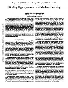
There are three high-level constructs in our architecture: nodes which contain and execute the activation functions, layers which contain the nodes and handle connections between layers and machines which contain the logic for the overarching algorithm. Each node in the bottom visible input layer reflects a feature in the dataset and for supervised models (predicts an outcome given an input) there is a visible output layer at the top of each configuration which performs classification. In unsupervised models (learns a model without a class label) as well for the internal layers (where applicable) in supervised models there is a hidden layer or layers, where the feature representation is learned.

Fig. 1. Machine Configurations within the Framework

Our architecture is implemented in Python and built upon Theano [7], [2] - a library for building and compiling symbolic mathematics expressions and GPU computation. The functions below are implemented for every algorithm. – initialise: instantiates model parameters (weights and biases), configures layers and nodes, and associates hyper-parameters with the architecture. – buildhypothesis: dependent on the classification type it builds a symbolic expression for the hypothesis function, giving the prediction hθ (xi ) = yˆi for the sample xi .

4

– buildcost: based on the classification type it creates symbolic expressions for: the cost J(θ) with regularisation2 (if applicable) and prediction error. – buildmodel: computes the gradient of the cost function with respect to the model parameters and uses this gradient to build a symbolic expression to update the parameters. It compiles these symbolic expressions into functions to train and (if applicable) pre-train the model. – train: optimises the cost function. Can be supervised (with respect to a class label) or unsupervised (no class label) depending on the algorithm. For the DBN it performs unsupervised pre-training and supervised fine-tuning (explained further in Section 2.5). – predict: uses the hypothesis function and model learned to predict an outcome, or reconstruct the data dependent on the algorithm. The following four machines: Regression, Multi-Layer Perceptron (MLP), Restricted Boltzman Machine (RBM) and Deep Belief Network (DBN) are currently implemented in our architecture and displayed in Figure 1. As our focus is not an in-depth discussion of the technical detail of these algorithms but their application to high dimensional clinical data and determining a DBNs best hyper-parameters via a step-wise optimisation of its constituent algorithms, we refer the reader to [4] for detailed technical information. 2.2

Regression

Three types of regression are currently implemented in our architecture: Linear, Logistic and Softmax regression. As our experiments only evaluate softmax regression, it will form the focus of our discussion. Softmax regression is a nonlinear multi-class classification algorithm which uses the softmax function for the hypothesis and the negative log likelihood function for the cost. It is used where class membership is mutually exclusive (sample can only belong to one class) to generate a probability of class membership from 1, . . . , K where K is the number of classes. In our architecture we train softmax regression with stochastic gradient descent. 2.3

Multi-Layer Perceptron

An MLP is a simple form of one hidden layer neural network, where latent and abstract features are learned in the hidden layer. As with the other machines in our architecture and for artificial neural networks (ANN) in general, each node in a hidden layer L(i) is connected to every node in layer L(i−1) and every node (i) (i) in L(i+1) . Each node n1 to nn in layer L(i) contains a non-linear activation function, which calculates a node’s activation energy. This value is propagated through the layers via the connections, a subset of which are shown in Figure 1. This process is called feed-forward propagation and is the hypothesis function for all shallow and deep feed-forward neural networks. 2

ensures features with large data values does not overly impact the model

5

Our MLP was trained with SGD and back-propagation. It is similar to training a regression model and uses the same cost function except the parameters in each layer must be updated with respect to the cost of the output. 2.4

Restricted Boltzmann Machine

An RBM is an energy-based, two-layer neural network. An RBM’s aim is to learn a model which occupies a low energy state over its visible and hidden layers for likely configurations of the data. The energy paradigm is an idea taken from particle physics and associates a scalar energy value (real-number) for every configuration of the variables in a dataset. Highly likely configurations of the data occupy low energy states, synonymous to low energy configurations of particles being most probable [4]. Training achieves this by maximising the probability of the training data in the hidden and visible layers by learning their joint probability distribution. This process gives a way of learning the abstract features that aid in prediction in MAAS. The RBM was trained with contrastive divergence [13] and MSGD. 2.5

Deep Belief Network

A Deep Belief Network is a deep ANN, meaning it can be successfully trained with more than one hidden layer and differs from RBMs and MLPs as such. Each subsequent layer learns a more abstract feature representation and increases the models predictive power. DBNs are generative models characterised by unsupervised pre-training and supervised fine-tuning. Unsupervised pre-training updates the weights in a greedy layer-wise fashion, where two layers at a time are trained as an RBM, where the hidden layer of one acts as the visible layer in the next. Supervised fine-tuning then adjusts these parameters with respect to an outcome via back-propagation, in much the same way as an MLP. Again, like an MLP it makes predictions via feed-forward propagation. Here we pre-trained the DBN with MSGD and fine-tuned with SGD.

3 3.1

Experimental Set-up and Design Dataset Preparation and Preprocessing

The MAAS dataset [16] is a longitudinal clinical trial which recorded biometric data on middle-aged individuals at 3 year intervals over 12 years. There are 3441 unique records and 1835 unique features spread throughout 86 ‘tests’ or study subsections. To remove the temporal nature of the data, only baseline data was analysed. To remove test level sparsity, a subset of the dataset was selected and the remaining sparsity was removed through deletion or mean imputation. The data was scaled to unit variance and categorised to one-hot encoded vectors so that it could be input into our DBN and RBM. The continuous data had 523 instances and 337 features, whereas the one-hot encoded categorical data had 523 instances and 3567 features.

6

3.2

Experimental Procedure and Parameter Initialisation

The optimum parameters for each machine were located via a process called grid search which tests a range of values to find wherein the optimum lies. Regression was used to determine the learning rate, regularisation term and fine-tune steps for the RBM, MLP and DBN; and the RBM and MLP were used to determine the number of nodes in the first and second hidden layers of the DBN respectively. The range searched for regularisation and learning rate was from 0.001 to 1, roughly divided into 10 gradations. Three values for steps of GD were tested: 100; 1000; and 10000 as we estimated any larger values would lead to over-fitting (not generalising well to new data) given the sample-size. All possible combinations were tested for both continuous and categorical data, giving 246 in total. The number of hidden nodes tested for both the RBM and MLP were 10, 30, 337, 900, 1300 and 2000. There were 337 features before categorisation therefore, any more than 2000 hidden nodes was deemed unnecessary. Each configuration was run twice (for categorical and continuous) in the MLP but 5 times each in the RBM (only categorical) as there were 5 epoch values (1, 5, 10, 15 and 20) being tested. Any more than 20 would have over-fit the data. Bias terms were initialised to zero for all models. From Glorot et. al [12], the MLP,qRBM, and DBN q weights were randomly initialised between the bounds: 6 6 [−4 f anin +f anout , 4 f anin +f anout ], whereas for regression the weights were randomly initialised without bounds. f anin is the number of inputs to and f anout is the number of outputs from a node. All experiments were run on a Dell Optiplex 790 running 64-bit Windows 7 Home Premium SP1 with an Intel Core i7-2600 quad-core 3.40 GHz CPU and 16.0GB of RAM. The code was developed in Python using the Enthought Canopy (1.4.1.1975) distribution of 64-bit Python 2.7.6 and developed in PyCharm 3.4.1 IDE, making use of the NumPy 1.8.1-1 and Theano 0.6.0.

4

Experimental Results and Analysis

4.1

Evaluation Metrics

– Ex.: Experiment number - a particular hyper-parameter configuration. Each number is an index into a list of the hyper-parameters being tested. – I. Cost Initial cost - negative log likelihood (NLL) cost of untrained model on training data – T. Cost: Training cost - NLL cost of trained model on training data – V. Cost: Validation cost - NLL cost of trained model on validation data – Tst. Cost: Test cost - NLL cost of trained model on the test set pos+true neg – Error: Prediction error achieved on the test set: 1 − ( true num predictions ) – Alpha: Learning rate, a coefficient for the model parameter updates which decides how big of a step to take in gradient descent. – Lambda: Regularisation parameter, determines how much to penalise large data values – Steps: Number of steps of stochastic gradient descent taken

7

– Data: Format of the data - cont. (continuous) or cat. (categorical one-hot encoded) – Epochs: Iterations through the dataset, 1 epoch = 1 complete iteration – Nodes: Number of nodes in each layer, visible-hidden1 -. . . -hiddenn (-output) 4.2

Regression: Search for DBN learning rate and regularisation term

Table 1 shows the results and hyper-parameter configurations for the ten best performing models in a series of grid-search experiments for regression. The models are ranked by the lowest negative log-likelihood found on the training data out of the 246 experiments performed. Table 1. Regression Learning Rate, Regularisation and Steps Grid Search Ex. 8-0-0 8-1-0 8-2-0 7-0-1 8-1-1 8-0-1 4-0-2 4-0-2 7-0-1 5-0-2

I. Cost 13.188452 4.925 7.608 21.066 9.718 9.200 12.103 16.553 6.193 11.149

T. cost 0.001 0.002 0.00334 0.003 0.004 0.003919 0.004 0.004 0.004 0.005

V. cost 45.818 7.725 22.615 6.449 35.637 15.913 14.097 16.351 8.180 9.223

Error 0.258 0.305 0.225 0.391 0.238 0.305 0.298 0.338 0.298 0.291

Alpha 0.9 0.9 0.9 0.3 0.9 0.9 0.03 0.03 0.3 0.09

Lambda 0.001 0.003 0.009 0.001 0.003 0.001 0.001 0.001 0.001 0.001

Steps 100 100 100 1000 1000 1000 10000 10000 1000 10000

Data cat. cat. cat. cat. cat. cat. cat. cont. cont. cat.

Experiments 8-1-0 and 7-0-1 achieved the best results for the categorical and continuous data respectively. 8-1-0 achieved a low training cost of 0.002, a validation cost of 7.725 and a test cost of 0.305. 7-0-1 achieved a slightly poorer result of 0.004, 8.180 and 2.816 for the same measures. Both experiments achieved the second lowest cost on the training data, but performed significantly better on the validation data, meaning these hyper-parameters generalised better. Models learned were not optimal, but given the amount of data available they were adequate as over 69% of the instances were correctly classified for the categorical data and just over 70% for the continuous data. Although the categorical data achieved a lower cost, the continuous data made better predictions. This suggests categorising the data helped remove noise but along with this the transformation eliminated some information relevant to modelling. Interestingly the best performing learning rate (alpha) is much higher for the categorical than the continuous data and ten times less iterations of gradient descent (GD) were required. Therefore gradient descent was far steeper for the categorical data as it converged and gave us the best parameters much faster than with the continuous, showing that one-hot encoded data can be modelled easier, building a predictive model in far less time.

8

4.3

RBM: To select optimum node count in first hidden layer of DBN

Table 2 shows the 10 highest scoring RBM model configurations out of 35 runs, ranked by the best reconstruction cost (closest to 0) achieved on training data. Table 2. RBM Layer 2 Hidden Nodes Grid Search Ex. 2-0 1-0 3-0 0-0 4-0 5-0 6-0 2-1 1-1 3-1

T. cost -68.719 -73.357 -75.110 -77.774 -98.590 -107.553 -141.144 -241.274 -241.527 -246.462

V. Cost Alpha Epochs Nodes -22.112 0.9 1 3567-100 -19.580 0.9 1 3567-30 -22.009 0.9 1 3567-337 -20.665 0.9 1 3567-10 -20.914 0.9 1 3567-900 -20.575 0.9 1 3567-1300 -22.532 0.9 1 3567-2000 -18.547 0.9 5 3567-100 -18.823 0.9 5 3567-30 -18.575 0.9 5 3567-337

The result of the best performing RBM configuration can be seen in bold in Table 2. It has 30 hidden nodes and went through 1 epoch of training. A node configuration of 100 units in the hidden layer achieved the best reconstruction cost of -68.719 on the training data, compared to the configuration with 30 hidden nodes which scored -73.357. The 30 hidden node configuration was determined to be the better architecture as it performed only slightly worse on the training data but it scored -19.580 on the validation set, performing better than every other configuration in the top 5 which measured in the 20’s. Therefore, the 30 hidden unit configuration generalises better to unseen data. The reconstruction cost achieved on the training data by Ex. 3-1 is far worse at -435.809, but the validation score is better at -17.977 due to the higher number of epochs. As the model iterates through the training data, more and more abstract features are learned so the model makes a better estimate at reconstructing unseen data. We want to learn the features that perform comparable on the training data as well as unseen data, therefore one training epoch gave the best performance. 4.4

MLP: To select optimum node count in final hidden layer of DBN

Table 3 shows the top 10 scoring experiments out of the 14 performed. Here, experiments 2 and 10 gave the best results achieving training, validation and test negative log likelihood costs of 0.17, 2.107, 0.76 and 0.842, 11.664, 0.974 respectively. From the above table it can be shown that ten hidden nodes - which is the smallest possible number of hidden nodes - gave the best results for both the categorical and continuous data. Further to this, the MLP improves upon the

9 Table 3. MLP Layer 3 Hidden Nodes Grid Search Ex. 2 4 6 8 1 10 12 3 14 5

I. Cost 2.389 5.319 13.466 33.467 11.247 64.252 73.305 30.256 121.088 99.757

T. cost 0.17 0.231 0.332 0.456 0.842 0.929 1.426 1.473 2.211 2.549

V. Cost 2.107 4.609 12.436 30.394 11.664 62.453 78.562 35.802 113.605 134.606

Error 0.232 0.225 0.225 0.238 0.291 0.232 0.212 0.318 0.219 0.616

Data Alpha Lambda Steps Nodes cont. 0.3 0.001 1000 337-10-2 cont. 0.3 0.001 1000 337-30-2 cont. 0.3 0.001 1000 337-100-2 cont. 0.3 0.001 1000 337-337-2 cat. 0.9 0.003 100 3567-10-2 cont. 0.3 0.001 1000 337-900-2 cont. 0.3 0.001 1000 337-1300-2 cat. 0.9 0.003 100 3567-30-2 cont. 0.3 0.001 1000 337-2000-2 cat. 0.9 0.003 100 3567-100-2

model found with regression for both data-types as the best performing MLP model was 76.8% accurate in its predictions for the continuous test data and 70.9% for the categorical. As a better predictive model was found through the MLP when we compare to regression, it would suggest that abstract features were learned in the hidden layer. Further to this, as the smallest available hidden node value performed best we conclude that the number of features particularly relevant to the outcome we are modelling are relatively low. It can again be seen from the results that that the continuous data lends itself to more powerful models in comparison to the categorical data and this can be put down to information being lost during transformation. 4.5

DBN: Comparing Configurations

Table 4 compares the results of the model learned with the hyper-parameters found through grid-search in earlier experiments (Ex. 6 - parameters in bold from previous experiments) with a randomly selected configuration (Ex. 1 - estimated to be a logical starting point) which was then tuned (Ex. 3, 4, 5) and two other configurations (Ex. 7, 8) which were an attempt to improve upon the results of Ex. 6. Tuning here refers to adjusting the hyper-parameters to find a better model. The heuristic used was to start the learning rate and training steps low and gradually increase one while observing if either the cost achieved or the accuracy improves. If the measures improve up to a point before deteriorating it can be seen that the global optimum has been overshot. Ex. 6 achieved the third best error rate on the test data. It immediately improved on 0.272 which was the lowest error rate achieved by picking a random initial configuration and tuning using technique outlined above. In fact, 0.272 was the best test error achievable without hyper-parameters found from previous experiments. Tuning improved the model up to a point (Ex. 2) before it degraded (Ex. 3, 4) and then again achieved previous levels of accuracy (Ex. 5).

10 Table 4. Comparing DBN Configurations Exp 1 2 3 4 5 6 7 8

I. Cost 2.582 1.653 3.837 0.694 0.916 2.818 9.236 0.748

T. cost 0.680 0.434 0.541 0.693 0.344 0.632 0.451 0.579

V. Cost 2.950 1.383 4.435 0.695 1.042 0.858 6.378 0.624

Error 0.536 0.272 0.305 0.616 0.272 0.265 0.238 0.245

Alpha 0.001 0.001 0.01 0.9 0.01 0.9 0.9 0.9

Lambda 0.003 0.003 0.003 0.003 0.003 0.003 0.003 0.003

Steps 3000 3000 3000 3000 1000 100 100 100

Nodes 3567-337-200-2000-10-2 3567-3567-200-10-2 3567-3567-200-10-2 3567-3567-200-10-2 3567-3567-200-10-2 3567-30-10-2 3567-337-10-2 3567-337-100-10-2

When choosing the estimated best starting point for the comparison configuration it was thought that more hidden layers would better model the data. The opposite was found when 2 hidden layers performed best. Interestingly, when a number of nodes the same as the number of features for the continuous data were inserted for the first hidden layer (Ex. 7) it improved on the test error from in Ex. 6. Our analysis is that an abstract feature representation similar to that of the original continuous data was learned in the first hidden layer. 0.238 - the lowest test error achieved (Ex. 7), improved upon on the error for the best categorical data model found with the MLP and approaches our previous best continuous data model score of 0.232 with the MLP. We concluded that this was due to the DBN learning a better feature representation in its hidden layers. This shows that a DBN with multiple-layers has great potential in learning a feature representation from text based datasets, given that this model was learned on only a small subset of the MAAS dataset and deep architectures have been shown to far outperform shallow models given enough data [24]. Therefore, it can be seen that performing a grid search on: the regression layer to find the learning rate and regularisation term; the RBM to find the number of nodes in the first hidden layer; and the MLP to find the number of nodes in the last hidden layer gave us a methodology for selecting a good starting point from which to determine the best hyper-parameter configuration for our deep network, at least in the case of a DBN.

5

Related Research

In [6], the authors introduce a random search method to find the best hyperparameter configuration for a DL architecture and compares their results to previous work [17] which - like our own - uses a multi-resolution grid-search coupled with a manual optimisation intervention element. In [6], they also carry out a series of simulation experiments where random search is compared to both grid-search and low discrepancy sequential methods. Their main contribution is a large series of non-simulated experiments which search for the best hyperparameters for a one-layer neural network and Deep Belief Network. These are

11

carried out on eight datasets in order to recreate and compare their experimental results with those obtained in [17]. Random search is found to outperform grid search on all datasets in a onelayer neural network, but for the DBN experiments, random and grid search perform comparably on four datasets with grid search outperforming on three datasets and random search finding the best model on the fourth dataset. In [6], the authors offer many reasons as to why random search is a better option but most hinge on the fact that they show that the hyper-parameter search space, although high-dimensional, has a low effective dimensionality. This means that although there are many parameters to tune, only a particular subset of these have a great effect on training the model and this subset is different for every dataset (also shown in the paper). This property leads to random search being more effective as it leaves fewer gaps in the search space and it does not require as many iterations in order to find the optimum hyper-parameter configuration. We chose grid and manual search for these exploratory experiments as it was shown to perform comparably to random search for a DBN. Both [6] and [17] chose to globally optimise the parameters of the entire DBN at once rather than incrementally tune its constituent parts. In other words, they do not optimise each model first where the results of the last set of experiments feed into the next. Contrary to an adaptive approach, which is the focus of our experiments and methodology. A second major issue is the analysis of high-dimensional data and feature selection [4], [5], [15] which has been extensively explored in a healthcare context [1], [3], [11]. In [11] and [1], both groups describe a methodology where features are selected in a two-step manually intensive fashion in order to learn predictive models. In these two approaches for selecting a feature representation in the health domain, shallow algorithms are utilised and high dimensional data is not encountered, where in one instance only nine features were modelled [11]. Furthermore, sometimes relevant features were completely eliminated which impacted on the performance of the model [1]. Finally, in the medical context, DBNs have been used for medical text classification [24], as well as to aid in medical decision making with electronic health recordds [18], but never for the analysis of clinical trial data. Neither [24] or [18] provide a methodology on how to choose the initial hyper-parameter configuration of a deep learning architecture. Furthermore, they use third party implementations of a DBN which do not allow for the extension with further algorithms, activation functions or hyper-parameter configurations. In [24], the authors utilise a single hidden layer in their DBN, which arguably is not a deep architecture, although they do employ a unsupervised pre-training step.

6

Conclusions and Future Work

Long term clinical studies present a number of key issues for data miners, of which high dimensionality, the identification of the principal features for prediction and distinguishing the optimal hyper-parameter configuration are most

12

prevalent. To address these issues, we developed a strategy which uses a configurable deep network to facilitate many combinations of attributes and multiple layers of attribute manipulation using regression, MLP, RBM and DBN models. Our framework demonstrated the ability to improve upon a randomly selected and tuned DBN configuration, as well the ability to configure many experimental runs in order to test hyper-parameter configurations found with grid-search. Furthermore, the MLP and DBN showed an ability to learn a feature representation in the hidden layers as an increased predictive accuracy was found compared to regression alone. We are now extending our CDN to make use of: more accurate imputations via hidden layer sampling; Gaussian hidden units for continuous data (avoiding one-hot encoding); random search for hyper-parameter optimisation; and dropconnect for improved accuracy [23].

References 1. Antonio Arauzo-Azofra, Jos Luis Aznarte, and Jos M. Bentez. Empirical study of feature selection methods based on individual feature evaluation for classification problems. Expert Systems with Applications, 38(7):8170 – 8177, 2011. 2. Fr´ed´eric Bastien, Pascal Lamblin, Razvan Pascanu, James Bergstra, Ian J. Goodfellow, Arnaud Bergeron, Nicolas Bouchard, and Yoshua Bengio. Theano: new features and speed improvements. Deep Learning and Unsupervised Feature Learning NIPS 2012 Workshop, 2012. 3. Riccardo Bellazzi and Blaz Zupan. Predictive data mining in clinical medicine: current issues and guidelines. International journal of medical informatics, 77(2):81– 97, 2008. R in 4. Yoshua Bengio. Learning deep architectures for ai. Foundations and trends Machine Learning, 2(1):1–127, 2009. 5. Yoshua Bengio, Aaron Courville, and Pascal Vincent. Representation learning: A review and new perspectives. Pattern Analysis and Machine Intelligence, IEEE Transactions on, 35(8):1798–1828, 2013. 6. James Bergstra and Yoshua Bengio. Random search for hyper-parameter optimization. J. Mach. Learn. Res., 13:281–305, February 2012. 7. James Bergstra, Olivier Breuleux, Fr´ed´eric Bastien, Pascal Lamblin, Razvan Pascanu, Guillaume Desjardins, Joseph Turian, David Warde-Farley, and Yoshua Bengio. Theano: a CPU and GPU math expression compiler. In Proceedings of the Python for Scientific Computing Conference (SciPy), June 2010. Oral Presentation. 8. Fabrice Camous, D´ onall McCann, and Mark Roantree. Capturing personal health data from wearable sensors. In Applications and the Internet, 2008. SAINT 2008. International Symposium on, pages 153–156. IEEE, 2008. 9. Kay Deckers, Martin PJ Boxtel, Olga JG Schiepers, Marjolein Vugt, Juan Luis Mu˜ noz S´ anchez, Kaarin J Anstey, Carol Brayne, Jean-Francois Dartigues, Knut Engedal, Miia Kivipelto, et al. Target risk factors for dementia prevention: a systematic review and delphi consensus study on the evidence from observational studies. International journal of geriatric psychiatry, 2014. 10. Neil Donnelly, Kate Irving, and Mark Roantree. Cooperation across multiple healthcare clinics on the cloud. In Distributed Applications and Interoperable Systems, pages 82–88. Springer, 2014.

13 11. Shobeir Fakhraei, Hamid Soltanian-Zadeh, Farshad Fotouhi, and Kost Elisevich. Confidence in medical decision making: application in temporal lobe epilepsy data mining. In Proceedings of the 2011 workshop on Data mining for medicine and healthcare, pages 60–63. ACM, 2011. 12. Xavier Glorot and Yoshua Bengio. Understanding the difficulty of training deep feedforward neural networks. In International conference on artificial intelligence and statistics, pages 249–256, 2010. 13. Geoffrey Hinton. A practical guide to training restricted boltzmann machines. Momentum, 9(1):926, 2010. 14. Geoffrey E Hinton, Simon Osindero, and Yee-Whye Teh. A fast learning algorithm for deep belief nets. Neural computation, 18(7):1527–1554, 2006. 15. Eric J Humphrey, Juan P Bello, and Yann LeCun. Feature learning and deep architectures: new directions for music informatics. Journal of Intelligent Information Systems, 41(3):461–481, 2013. 16. van Boxtel M.P.J. Ponds R.H.W.M Jolles J., Houx P.J. The Maastricht Ageing Study: Determinants of. Maastricht: Neuropsych Publishers, 1995. 17. Hugo Larochelle, Dumitru Erhan, Aaron Courville, James Bergstra, and Yoshua Bengio. An empirical evaluation of deep architectures on problems with many factors of variation. In Proceedings of the 24th International Conference on Machine Learning, ICML ’07, pages 473–480, New York, NY, USA, 2007. ACM. 18. Znaonui Liang, Gang Zhang, Jimmy Xiangji Huang, and Qmming Vivian Hu. Deep learning for healthcare decision making with emrs. In Bioinformatics and Biomedicine (BIBM), 2014 IEEE International Conference on, pages 556–559. IEEE, 2014. 19. Mark Roantree, Jim ODonoghue, Noel OKelly, Maria Pierce, Kate Irving, Martin Van Boxtel, and Sebastian K¨ ohler. Mapping longitudinal studies to risk factors in an ontology for dementia. Health Informatics Journal, pages 1–13, 2015. 20. Mark Roantree, Jie Shi, Paolo Cappellari, Martin F. OConnor, Michael Whelan, and Niall Moyna. Data transformation and query management in personal health sensor networks. Journal of Network and Computer Applications, 35(4):1191 – 1202, 2012. Intelligent Algorithms for Data-Centric Sensor Networks. 21. Ruslan Salakhutdinov and Geoffrey E Hinton. Deep boltzmann machines. In International Conference on Artificial Intelligence and Statistics, pages 448–455, 2009. 22. Martin PJ van Boxtel, Frank Buntinx, Peter J Houx, Job FM Metsemakers, Andr´e Knottnerus, and Jellemer Jolles. The relation between morbidity and cognitive performance in a normal aging population. The Journals of Gerontology Series A: Biological Sciences and Medical Sciences, 53(2):M147–M154, 1998. 23. Li Wan, Matthew Zeiler, Sixin Zhang, Yann L Cun, and Rob Fergus. Regularization of neural networks using dropconnect. In Proceedings of the 30th International Conference on Machine Learning (ICML-13), pages 1058–1066, 2013. 24. Antonio Jimeno Yepes, Andrew MacKinlay, Justin Bedo, Rahil Garnavi, and Qiang Chen. Deep belief networks and biomedical text categorisation. In Australasian Language Technology Association Workshop 2014, page 123.