ate candidate control actions using a technique called hindsight optimization. In hindsight optimization, the finite-horizon âutilityâ achievable from a given system.
A Framework for Simulation-based Network Control via Hindsight Optimization Edwin K. P. Chong, Robert L. Givan, and Hyeong Soo Chang School of Electrical and Computer Engineering Purdue University, West Lafayette, IN 47907-1285 E-mail: {echong,givan,hyeong}@ecn.purdue.edu Abstract We describe a novel approach for designing network control algorithms that incorporate traffic models. Traffic models can be viewed as stochastic predictions about the future network state, and can be used to generate traces of potential future network behavior. Our approach is to use such traces to heuristically evaluate candidate control actions using a technique called hindsight optimization. In hindsight optimization, the finite-horizon “utility” achievable from a given system state is estimated by averaging estimates obtained from a number of traces starting at the state. For each trace, the utility value of the state is estimated by determining the optimal “hindsight control”—this is the control that would be applied by an optimal controller that somehow “knew” the whole trace beforehand—and then measuring the utility obtained under that control. Averaging over many samples then gives a simulation-based “hindsight-optimal” utility for the starting state that upper bounds the true utility value of the state. This technique for estimating state utility can then be used to select the control—simply select the control that gives the highest utility. Our hindsight-optimization approach to designing simulation-based control algorithms can be applied to a wide variety of network decision problems. We present empirical results showing effectiveness for two example control problems— multiclass scheduling and congestion control. 1 Introduction Because of the stochastic nature of network traffic, both at the packet and at the call or flow level, most network decision problems are complex stochastic control problems. These problems can be formalized as Markov decision processes (MDPs) with extremely large state spaces, with the added complexity that the current system state is never fully known to the control process. In such “partially observable” MDPs (POMDPs), finding the optimal control is known to be very difficult in general (see, e.g., [12]). Recent decision-theory research [15], [10] has shown that simulating system behavior can provide a princiResearch supported in part by NSF under grant ECS-9501652 and by DARPA/ITO under grant F19628-98-C-0051.
pled way to find an optimal policy within asymptotically slowly-growing time bounds (i.e., the sampling method runtime does not grow exponentially with problem size). However, these techniques still require absurdly large amounts of simulation to get bounds on policy values that can be used in controlling a network in most common network decision problems. In this paper, we describe an alternative and more effective paradigm for applying simulation to POMDP control problems. Under this paradigm, we do not simulate a policy, but instead use a simulation model to generate traces of the stochasticity in the system (typically traffic traces drawn from a traffic model). For each such trace, we can then compute the optimal control. We call this the “hindsight control,” because the true control problem being faced does not allow us to know the traffic trace—the control problem when knowing the trace is like computing what we wish we had done after encountering the traffic, i.e., the “hindsight” control. For each trace, the hindsight control can be used to determine the “hindsight-optimal value” of the trace—that achieved under the hindsight control. We take this value as a heuristic estimate (in general it is an upper bound) of the value that we can accrue if we encounter that trace. Averaging the hindsight-optimal values over many traces, we get an upper bound on the optimal expected value achievable from the current state. Given this means of estimating optimal values, familiar decision-theoretic techniques (described below) then select an action based on knowledge of the current utility of each action (the “Q-values”). Hindsight optimization provides a general approach to incorporating simulation in decision-making, yielding in turn a general means for creating control policies that incorporate traffic models representing expectations about the future traffic. This technique can be applied to a wide variety of control problems faced in the networking context. We describe below (in Section 3) a proof-of-concept implementation of this approach for two simple problems: multiclass scheduling and congestion control. We have empirically evaluated our implementations and have demonstrated substantially superior performance when comparing to previous control policies. The hindsight-optimization approach exploits the particular structure of some net-
work control problems, making it possible to obtain superior performance. In particular, the technique appears to work best in situations where the randomness is “exogenous”—i.e., the future traffic does not depend on the current control. 2 Hindsight Optimization Problem Framework. Our problem setting follows that of standard Markov decision processes (MDPs). Here we briefly describe the setting (for more details, see [2]). Let X be a set of system states. At each state x ∈ X, we take an action (or apply a control) a in a set A(x) of feasible action choices. If we take action a at state x, we receive a reward of R(x, a), and the next state y is chosen according to a state-transition probability P (x, y, a) (in networking applications, the randomness of the next state is typically due to random traffic). If we start at state x and apply a sequence of actions a0 , a1 , a2 , . . ., resulting in a sequence of states x1 , x2 , . . ., then the total reward �P value over a �horizon H−1 of H time steps is VH (x) = E i=0 R(xi , ai ) where the expectation is taken over possible (random) state sequences, and x0 = x. In the standard problem formulation, we are interested in action choices that are determined by “state feedback”—if we are in state xi at time i, then we set ai = µi (xi ), where µi is a statefeedback map. The sequence π = {µ0 , µ1 , . . .} is called a policy. An optimal policy π ∗ = {µ∗0 , µ∗1 , . . .} is one that maximizes the total value. We denote the associated optimal value by VH∗ . ∗ We write Qi (x, a) = R(x, a) + E(Vi−1 (y)), where the expectation is with respect to the next state y, and ∗ Vi−1 (y) is the optimal value over i−1 time steps starting at state y. The main result in Markov decision theory states that VH∗ (x) = maxa∈A(x) QH (x, a). Moreover, the policy defined by µ∗i (x) = arg maxa∈A(x) QH−i (x, a) is an optimal policy. In particular, for a fixed horizon H, the action a∗ = µ∗0 (x) = arg maxa∈A(x) QH (x, a) is an optimal “current” action in maximizing the total value VH (x). In practice we do not know QH (x, a)—the best we can hope for is to estimate these values. The hindsight-optimization approach is based on the following rationale. At each time step, we select the action a∗ just described using an estimate of the values QH (x, a), for a fixed horizon H. For convenience, we henceforth drop the subscript H and refer to the values of Q(x, a) as the “Q-values.” For a given state x and an action a, we estimate the value of Q(x, a) as follows. We first generate traces of possible future “randomness” over a horizon of H (in the case of network control problems, these are typically traces of future traffic), starting from state x. For each possible trace of the future, we compute the reward accumulated by taking action a at time step 0 followed by the trace-specific optimal sequence of actions a∗1 , a∗2 , . . . for the remaining horizon of H − 1 in the trace. This optimal sequence of actions corresponds to one that would be taken by a
controller with “hindsight” knowledge of uncertainties in the future. The optimal accumulated reward along a given trace is called the hindsight-optimal value of that trace. We use the average of the hindsight-optimal values over the set of generated traces as our estimate of the value of Q(x, a). Once we have estimated Q(x, a) for all values of a ∈ A(x), we can then select the action a∗ to be applied using the equation defining a∗ above. This approach of applying a “moving-horizon” control solution in an on-line fashion is common in the optimalcontrol literature, (e.g. receding-horizon control [13]). Formally, our procedure for estimating the Q-values ˆ a) as an estimate of uses the following quantity Q(x, ˆ Q(x, a): Q(x, a) = R(x, a) + E(VˆH−1 (x1 )), where ! H−1 X ˆ VH−1 (x1 ) = E max R(xi , ai ) x1 . a1 ,a2 ,... i=1
Comparing the above with the equation Q(x, a) = ∗ R(x, a) + E(VH−1 (x1 )), where ∗ (x1 ) VH−1
= max E µ1 ,µ2 ,...
H−1 X i=1
! R(xi , µi (xi )) x1 ,
ˆ a) is an upper it is easy to see that our estimate Q(x, bound of Q(x, a). Note that the “max” in the definition of VˆH−1 is over sequences of actions, due to the ability (in VˆH−1 ) to apply tailored action sequences to different stochastic futures. In contrast, the “max” in ∗ VH−1 above occurs outside the expectation, requiring a single policy to be selected for all futures. In a general decision problem, there is no reason to ˆ upper bound is at all tight (it can suppose that the Q be arbitrarily loose). Even in the network-control problems we consider, we expect that this upper bound may often be loose. However, because we are interested in Q-values only to rank candidate control actions, we only need the upper bounds to preserve the relative value at different states. Our initial results below for selected problems illustrate that these relative values are often ˆ upper bounds. The problems for well reflected in the Q ˆ upper bound to help us which we most expect the Q make decisions are those that involve “exogenous” randomness; i.e., problems where the randomness is not a function of the control, such as networks where the traffic does not depend on the control decision. The key step in our approach is selecting the hindsight-optimal sequence of control actions, given a particular trace of future randomness. In general this can be a very hard optimization problem; however, for typical network control tasks, this problem is both solvable and novel—limited work has been done on optimal network decision-making with known traffic traces. The utility estimates obtained by this technique may not converge to the true utility with large sample size— these are heuristic estimates that must be evaluated empirically by the performance of the resulting policy.
Network Partial Observation State Estimation
Selected Action Candidate Action
Action Selection
Traffic Traces
Hindsight-optimal Values
Hindsight Optimizer
...
...
State Estimate
Traffic Simulation
Q-value Estimate
Averaging
Action Evaluator
Figure 1: Basic control architecture Control Architecture. The basic control architecture of our framework is shown in Figure 1. The main components of the framework (the decision-making module) are the action evaluator and action selector, which use system-state estimates together with a traffic simulator to select control actions to be applied to the network. As will be described further below, because we only have partial observations of the system, we do not have access to actual system states but only estimates of them. The state variable x from our previous description must then be interpreted as a state estimate. Indeed, standard MDP theory can be applied to the partially-observed case by incorporating the state estimate distribution into the state space (see [2]). The controller takes as input a state estimate reflecting what is known about the hidden state of the traffic sources—this state estimate and its maintenance over time depend on the particular traffic model used. For example, if the traffic model is a Markov-modulated Bernoulli process, the state estimate is a probability distribution over the hidden Markov state space, and the update rule is given by POMDP theory and is essentially a form of Bayes’ rule for incorporating new observations. (Put more concretely, each time new traffic arrives, Bayes’ rule is used to update our expectations about future traffic based on our traffic model.) The decision-making module (action selection plus action evaluation) uses the state estimate to inform the traffic simulations used to select the control action, shown as the output of the module fed back into the network. The decision-making component is dominated by the action evaluator. This module first uses the traffic model (with the state estimate) to generate potential future traffic traces. The hindsight optimizer then computes the value obtainable by a controller encountering each trace with foreknowledge (or, equivalently, the value obtainable by a “revisionist” hindsight controller looking back on the traffic). The values for the different traces are then averaged, giving the overall value obtainable. The module shown is labeled an “action evaluator” because it accepts as input a “candidate action” to be evaluated—this evaluation is done by requiring that the selected control in the hindsight optimizer begin with that action, as described in the previous section. The action evaluator returns an estimate of the utility of taking the candidate action a ˆ a)). This same estimation process at state x (i.e., Q(x, is performed for each candidate action, and the action
with the highest utility estimate is selected. We have found it critical for the simulation traces used in evaluating different candidate actions for comparison against one another be the same traces— otherwise far more traces are needed for the comparison. Our interest in the relative rather than exact utility of the actions allows us to tolerate less accurate estimates when the inaccuracy is systematic across all actions. So, our technique allows savings in simulation time by focusing on the relative utility—similar to the benefits of common-random-numbers simulation in perturbation analysis [9] (see also [3]). State Estimation: Stochastic traffic models implicitly describe probability distributions over possible future traffic sequences. With many traffic models, these distributions change over time depending on the actual traffic. For example, if the model indicates we are expecting a burst of traffic in the near future with high likelihood, and then such a burst arrives, we may no longer be expecting such a burst (i.e., traffic sequences containing such bursts will be assigned a low probability by the model after the burst arrives, but a high probability before the burst). Maintaining the traffic model during traffic arrivals is the task of state estimation. In our initial work in this framework, we have used Markov-modulated Bernoulli Process (MMBP) traffic models (e.g., [7], [14]). These models can easily represent a wide variety of interesting traffic patterns, including self-similar traffic. An MMBP traffic model is a discrete time model given by providing a finite set S of traffic generation states, with a transition probability matrix T giving for each pair of states s1 and s2 from S the probability of transitioning from s1 to s2 at each time step spent in s1 . Associated with each state s ∈ S is a Bernoulli process Bs governing traffic generation for each time step spent in state s. This process is given by specifying a single probability of generating a packet during each time step (when multiple simultaneous arrivals are allowed, a distribution over the possible number of arrivals must be given). While we currently model network traffic with a state-based model such as an MMBP traffic model, we assume that the controller does not have access to any direct observation of the current state of the traffic model. The only way the controller can gain any knowledge of this state is by observing the traffic generated and performing state estimation. In this case, a state estimate is a probability distribution over the possible traffic generation states (all those in S). This estimate is easily updated using Bayes’ rule after each time step of traffic arrivals, given knowledge of the transition probabilities T and the state-associated Bernoulli processes Bs . Note that the state estimation process relies on the controller having knowledge of the traffic model itself: this knowledge is expected to derive either from a model inference algorithm (such as the expectation maximization (EM) algorithm, widely used in hiddenMarkov-model estimation problems (e.g., [17])[18]), or
from call or flow-related information (possibly selected from a library of generic traffic models representing different types of call or flow), or possibly even from policing of the traffic source. Action Evaluation: The action evaluation module is the heart of our control framework. This module accepts a state estimate and a candidate action as input, and must return a Q-value estimate reflecting the expected utility achieved by taking that action assuming optimal behavior thereafter. Accurate calculation of Q-values is known to be intractable in general in partially observable contexts (i.e., where state estimation must be used rather than direct knowledge of the underlying state), and is expensive even in fully-observable contexts where the state space is very large. However, because we are only using the Q-values to select an action to perform, we only care about the relative values, not necessarily about the accuracy of the values. For these reasons, it may suffice to use our previously described heuristic method of Q-value estimation, focusing on preserving the relative Q-values where possible. Recall that our approach is to use the state estimate provided to generate simulation traces of the stochasticity in the system. In simple cases where the control is open-loop, this trace does not depend on the selected control actions and often simply amounts to a likely future traffic sequence. Closed-loop control problems (e.g., those resulting from models incorporating TCP protocol effects) are more complex and are subjects of further ongoing research to broaden our framework. Once we have simulation traces describing “possible futures” for the system, we derive an approximate Qvalue for taking the candidate action by assuming that we start with that action, and then solving for the optimal subsequent control for each simulation trace and measuring the value attained under that control. By averaging these values over the different traces, we get what we call the hindsight-optimal Q-value for the candidate action. This is the value we expect to obtain if we start with the candidate action and our controller presciently knows the future traffic. It is important to note that we use the simulation traces by assuming for each one (in turn) that the trace is the actual traffic, and then computing the optimal control for that traffic. This assumption often makes fast analysis possible. Action Selection: In the simplest case, the action selection portion of our framework involves using the action evaluator to estimate the Q-value for each candidate action, and then selecting the action with the highest estimate. This technique is used in the scheduling example described in Section 3 below. However, a number of issues can complicate this plan. In many network problems, the control decision must be made at a very fine timescale-too fine to allow for repeated simulation and even very simple simulation analysis. In these situations, the action selection technique just described will be too expensive. We intend to design control for such problems by design-
ing a parameterized policy and using the hindsightoptimization technique to select the best parameter settings at a coarser timescale. In this case, the action selection task is to select a parameter setting to be used by the parameterized policy for a period of time until a new selection is made (thus giving a mechanism for automatically adapting the parameter setting to changing traffic conditions as reflected in the traffic model). An additional issue that arises when the space of candidate actions is quite large (e.g., the space of possible parameter settings for a parameterized policy, as just described). In this case, it is not possible to try every possible candidate action—instead, it is necessary to use search techniques such as gradient ascent to find a locally hindsight-optimal action by using hindsightoptimization to evaluate some but not all of the candidate actions. This technique is used in the congestion control example discussed below. The details of this approach will depend heavily on the structure of the action space for the problem at hand. Adaptation: The block diagram in Figure 1 reflects the basic operation of a hindsight-optimization-based controller. Implicit in this operation is the presence of a traffic model that is informing the traffic simulation block. Therefore, it is quite natural to convert a hindsight-optimization controller into an adaptive controller by adding a traffic model inference module that updates the traffic model periodically. The resulting controller can be expected to select control based on an ongoing and changing estimate of the expected future traffic patterns. Such a controller will react flexibly to a variety of changing conditions including both unexpected network faults and changing congestion conditions, providing a form of adaptive fault tolerance automatically at each control point in the network structure. Related Work: As mentioned in Section 1, the recent decision-theoretic work of [15] and [10] provide an impractical alternative way of finding optimal policies using simulation. Recent work by Bertsekas et al. on rollout algorithms also provide a means of using simulations to find “good” control actions [3, 4]. However, that work was formulated for the simpler fullyobservable problem domain, rather than the partiallyobservable domain common in network control. Also, the rollout approach relies on starting with a good heuristic policy for the control problem being considered, in contrast with our approach. Interestingly, while our hindsight approach provides an upper bound on the Q-values, the rollout approach provides a lower bound. Together such upper and lower bound values may yield useful information on the accuracy of our Q-value approximation, suggesting the possibility of combining the rollout approach with ours in a natural way. 3 Examples Multiclass Scheduling. In this section we discuss a network control problem that we have studied within our framework. We considered the scheduling problem
10000 9000 8000
Cumulative weighted loss
for packet networks with multiple classes of traffic with associated deadlines. For this example, we assumed discrete time and fixed-size packets falling into a small finite number of classes, where each class has an associated weight. The objective of the scheduler here is to minimize the weighted loss of packets, where a packet is lost if it is not served before its deadline. As a baseline for comparison, we considered two simple schedulers for this problem, along with a third scheduler that we designed without using simulation. The simple schedulers were: (1) earliest-deadline-first (EDF), which ignores the classes and serves the soonestto-expire packet; and static-priority (SP), which ignores deadlines and always serves the highest weighted outstanding packet. The scheduler we designed without simulation is a greedy scheduler called current-minloss (CM), which selects a packet so as to minimize weighted loss on those packets already in the queue if no further packets arrive (see [6] for details). Note that both EDF and CM are throughput optimal scheduling policies— these policies minimize idle time, always serving as many packets as possible over any time interval and traffic (see [8]). SP can fail to have this property by focusing exclusively on class weight. We then designed a hindsight-optimizing (HO) scheduler, which uses the techniques of this paper to estimate the impact of modeled future traffic on the scheduling decision. The framework requires solving the offline problem in order to analyze simulation traces-in this case, that problem is to find the optimal schedule for a multiclass traffic stream with deadlines when that traffic is known in advance. We designed a solution to this problem that we call the “Prescient Minloss” algorithm (see [5] for details). This solution works by considering the packets from highest weight to lowest weight, and creating a schedule by adding each packet as it is considered at the latest possible time in the schedule. Adding a packet to the schedule may require shuffling the packets already in the schedule to earlier times-as long as no packet is shuffled to a time before its arrival. If there is no way to shuffle packets in the schedule to allow the addition of a packet when it is considered, then the packet is dropped. We have proven that this approach yields an optimal schedule for the specific traffic in the simulation trace. The hindsight-optimization technique described in Section 2 provides a natural means to extend this algorithm for offline scheduling into an online scheduler that uses simulation and traffic modeling. Each simulation trace is analyzed using the offline algorithm for each candidate action, to give an “optimistic” estimate of the value obtainable after the action (an optimistic Q-value estimate). The action with the best estimate (averaged over the different traces) is selected and performed. For this example, the simulation-based decision-making is repeated at each time step. The resulting control policy is called the hindsight-optimizing (HO) policy. Figure 2 shows results for comparing these four
7000 6000 5000 4000 3000 EDF SP CM HO
2000 1000 0 0
2
4
6
8
10 Time
12
14
16
18 4
x 10
Figure 2: Weighted packet loss for four schedulers schedulers on this multiclass scheduling problem with deadlines. The graphs show the cumulative weighted packet loss over time for each scheduler against two different traffic sources. These results were obtained using the NS simulator to evaluate the four schedulers for the problem. These results show that the simple schedulers fail completely to control weighted loss. The greedy CM scheduler we designed achieves a more reasonable weighted loss, and our hindsight-optimizing HO policy achieves a further substantial improvement by incorporating an accurate traffic model using our techniques. Congestion Control. We have also tested our control framework for a multi-source congestion control scheme, in work with Gang Wu. A full description of our results on congestion control is presented in [19]; here we present a brief summary. The control problem involves a bottleneck node in a network through which we assume there are a number of fully controllable sources attempting to transmit data—these sources are located at various control delays from the bottleneck node. We assume Markov-modulated cross-traffic affecting the available bandwidth at the bottleneck node, and attempt to select flow rates for the sources to maximize the (weighted) difference between throughput achieved and delay experienced at the bottleneck node, with a fairness penalty term applied to encourage fair allocation of bandwidth among the sources. In our empirical evaluation of the congestion control scheme, we used the network simulator “NS” (currently available from Lawrence Berkeley National Laboratory’s website at http://www-mash.cs.berkeley.edu/). The simulated network comprises three controlled traffic sources (transimitting low-priority traffic), one uncontrolled “cross-traffic” source (transmitting highpriority traffic), one bottleneck node, and one sink node. Traffic from all the sources, controlled or uncontrolled, goes through the bottleneck node to the sink node via a 55 Mbps link. All other links are of bandwidth 155 Mbps. The round-trip delays from the three controlled sources to the bottleneck node are nonnegligible: they are 20, 30, and 40 ms. The uncontrolled node generates traffic consisting of 10 identical two-state on/off traffic flows, each having a mean rate of 2.2 Mbps. In tests below, we will be varying the (on and off) rates to have different variation of the aggre-
1
1000
ing the interaction of the TCP protocol with network control. Further, by incorporating online traffic model inference techniques into the framework, we hope to automatically extend the control algorithms designed using our framework to adaptive algorithms that react to changing traffic conditions, including hostile attacks and unforeseeable congestion.
0.95 800
0.9
Delay (secs.)
Utilization
0.85 0.8 0.75 0.7 0.65 0.6 0.55 0
HO PD−50 PD−10 PD−1 20
HO PD−50 PD−10 PD−1
600
400
200
40
Variance (Mbps2)
60
80
0 0
20
40
60
80
Variance (Mbps2)
References
Figure 3: Utilization and delay for four controllers gated traffic rate but at the same time keep the same mean. This allows us to study the impact of the cross traffic variance on the congestion controller. Our congestion controller, residing at the bottleneck node, computes rate commands based on the bandwidth left unused by the high-priority cross-traffic and relays them to the controlled sources. The controller is implemented within the hindsight optimization framework, using a gradient ascent method to find a locally “hindsight optimal” action in the continuous action space. We note that the hindsight optimizing controller here exploits an accurate stochastic model of the cross traffic, which is not used by the competing controllers. The goal is to show that this model can be used to improve the provision of high utilization, low delay, low packet loss rate, while maintaining fairness. Figure 3 shows bottleneck-link utilization and delay experienced for our technique and three competing PD-style controllers [11, 1] on this problem, as the variance of the cross-traffic model is increased. These plots show that our scheme provides the desired balance between utilization and delay—the only comparable PD controller with respect to delay has highly unacceptable throughout. Space precludes showing results that demonstrate the new technique dramatically reduces packet loss and achieves reasonable fairness (but somewhat less fairness than PD controllers). 4 Summary and Conclusions We presented a novel paradigm for designing online simulation-based control algorithms. However, much remains to be explored in our framework. Perhaps the most significant research task is to determine the breadth of applicability and select most fruitful areas of application of the new approach; a closely related task is to develop a better analytical understanding of the new paradigm. The experimental work summarized above represents a preliminary proof-of-concept for this new idea, but cannot be viewed as a measure of its potential generality. We plan to exploit fully the potential impact of this technique by applying it to a wide range of network control problems at varying granularities of network behavior; we further plan to study the interaction between our technique and self-similar and multifractal traffic models (e.g., [16]) and expand the applicability of our approach by considering closedloop control questions such as those raised by consider-
[1] L. Benmohamed and S. M. Meerkov, “Feedback control of congestion in packet switching networks: The case of a single congested node,” IEEE/ACM Trans. Networking, vol. 1, no. 6, pp. 693–707, Dec. 1993. [2] D. P. Bertsekas, Dynamic Programming and Optimal Control, Vol. 1 and 2. Athena Scientific, 1995. [3] D. P. Bertsekas, “Differential Training of Rollout Policies,” in Proc. 35th Allerton Conference on Communication, Control, and Computing, October 1997. [4] D. P. Bertsekas and D. A. Castanon, “Rollout Algorithms for Stochastic Scheduling Problems,” J. of Heuristics, Vol. 5, pp. 89–108, 1999. [5] H. S. Chang, R. Givan, and E. K. P. Chong, “On-line scheduling via sampling,” in Proc. 5th Int. Conf. on Artificial Intelligence Planning and Scheduling (AIPS2000), April 11–15, pp. 62–71, 2000. [6] R. Givan, E. K. P. Chong, and H. S. Chang, “Scheduling multiclass packet streams to minimize weighted loss,” unpublished manuscript, 2000. [7] W. Fischer and K. Meier-Hellstern, “The Markovmodulated Poisson process (MMPP) cookbook,” Perf. Evaluation, Vol. 18, pp. 149–171, 1992. [8] B. Hajek and P. Seri, “On causal scheduling of multiclass traffic with deadlines,” in Proc. IEEE Int. Symp. on Infor. Th., pp. 166, 1998. [9] Y.-C. Ho and X.-R. Cao, Perturbation Analysis of Discrete Event Dynamic Systems, Kluwer, 1991. [10] M. Kearns, Y. Mansour, and A. Y. Ng, “Approximate Planning in Large POMDPs via Reusable Trajectories,” in Adv. in Neural Infor. Proc. Sys., S. A. Solla, T. K. Leen, and K. R. Muller, eds., MIT Press, 2000. [11] A. Kolarov and G. Ramamurthy, “A control-theoretic approach to the design of an explicit rate controller for ABR service,” IEEE/ACM Trans. Networking, vol. 7, no. 5, pp. 741–753, Oct. 1999. [12] M. L. Littman, Algorithms for Sequential Decision Making. Ph.D. dissertation and Technical Report CS-96-09, Brown University, Computer Science Dept., Providence, RI, March 1996. [13] D. Q. Mayne and H. Michalska, “Receding horizon control of nonlinear systems,” IEEE Trans. Auto. Contr., vol. 35, no. 7, pp. 814–824, Jul. 1990. [14] H. Michiel and K. Laevens, “Teletraffic engineering in a broad-band era,” Proc. IEEE, vol. 85, No. 12, pp. 2007–2032, 1997. [15] D. A. McAllester and S. Singh, “Approximate Planning for Factored POMDPs using Belief State Simplification,” in Proc. 15th Annual Conf. on Uncertainty in AI, pp. 409–416, 1999. [16] K. Park and W. Willinger (eds.), Self-Similar Network Traffic and Performance Evaluation, Wiley Interscience, 1999. [17] L. R. Rabiner, “A tutorial on hidden Markov models and selected applications in speech recognition,” Proc. IEEE, Vol. 77, No. 2, pp. 257–285, 1989. [18] J. W. Turin, “Fitting stochastic automata via the EM algorithm”, Stochastic Models, vol. 12, pp. 405–424, 1996. [19] G. Wu, E. K. P. Chong, and R. Givan, Jr. Burst-level Congestion Control Using Hindsight Optimization, unpublished manuscript, School of Electrical and Computer Engineering, Purdue University, 2000. (available at http://dynamo.ecn.purdue.edu/ ngi/)