. VRML
A Framework for Streaming Geometry in VRML S
everal factors currently limit the size of Virtual Reality Modeling Language (VRML) models that can be effectively visualized over the Web. Principal factors include network bandwidth limitations and inefficient encoding schemes for geometry and associated properties. The delays caused by these factors reduce the attractiveness of using VRML for a large range of virtual reality models, CAD data, and scientific visualizations. The Moving Pictures We introduce a framework Expert Group’s MPEG-4 addresses the problem of efficiently encoding for streaming geometry in VRML scene graphs. MPEG-4 version 2 contains a 3D mesh coding VRML that eliminates the toolkit to compress IndexedFaceSet and LOD nodes, featuring need to perform complete progressive transmission.1 downloads of geometric In this article we propose a framework to mitigate the effects on users of long delays in delivering VRML models before starting to content. Our solution is general and can work independently of VRML. display them. We exploit the powerful prototyping mechanisms in VRML2 to illustrate how our techniques might be used to stream geometric content in a VRML environment. Our framework for the progressive transmission of geometry has three main parts, as follows: 1. a process to generate multiple levels-of-detail (LODs), 2. a transmission process (preferably in compressed form), and 3. a data structure for receiving and exploiting the LODs generated in the first part and transmitted in the second. The processes in parts 1 and 2 have already received considerable attention (see below and the sidebars). In this article we’ll concentrate on a solution for part 3. Our basic contribution in this article is a flexible LOD storage scheme, which we refer to as a progressive multi-
68
March/April 1999
André Guéziec, Gabriel Taubin, and Bill Horn IBM T.J.Watson Research Center Francis Lazarus IRCOM-SIC and University of Poitiers
level mesh. This scheme, primarily intended as a data structure in memory, has a low memory footprint and provides easy access to the various LODs (thus suitable for efficient rendering). This representation is not tied to a particular automated polygon reduction tool. In fact, we can use the output of any polygon reduction algorithm based on vertex clustering (including the edge collapse operations used in several algorithms). The progressive multilevel mesh complements compression techniques such as those developed by Deering,3 Hoppe,4 Taubin et al.,5 or Gumbold and Strasser.6 We discuss the integration of some of these compression techniques. However, for the sake of simplicity, we use a simple file format to describe the algorithm, which we’ll explain later. Transmitting or storing a mesh in this file format (or compressing it with standard tools such as gzip) proves useful only in situations where no available geometric compression methods will serve. (For instance, when encoding arbitrary vertex clusterings that change the topology and introduce a nonmanifold connectivity). In our approach, we partition the vertices and triangles of the mesh into several LODs by assigning an integer level to each vertex and triangle. We define and use vertex representatives to cause certain vertices—depending on the selected LOD—to be represented by another, substitute vertex. Not all vertices have representatives. Or, more precisely, a vertex may be represented by itself. Representatives can be stored in a single array with one entry per vertex. Using the PROTO mechanism of VRML and a script node executing Java code, we implemented a new VRML node to support this representation. A live demo is currently available on the Web at http://www .research.ibm.com/people/g/gueziec (where you can access relevant VRML files and Java bytecode). Figure 1 shows snapshots of our VRML implementation (an earlier version of this demo appeared at VRML 987). Note the LOD can be changed interactively after (and even during) progressive loading. When restricting ourselves to LODs produced using the familiar edge-collapse operations (as Ronfard and
0272-1716/99/$10.00 © 1999 IEEE
.
1 Snapshots of our VRML implementation using a horse model (original model provided by Rhythm & Hues Studios). LODs with (a) 247, (b) 665, (c) 1,519 and (d) 4,350 triangles are accessed interactively on a Pentium 133MHz laptop PC using a VRML browser.
Triangular Meshes, LODs, and Edge Collapses A polygonal surface is often represented with a triangular mesh, composed of a set of vertices and a set of triangles, each triangle being a triplet of vertex references. In addition, triangular meshes have a number of vertex or triangle properties such as color, normal, or texture coordinates. A corner is a couple (triangle, vertex of triangle). An edge is a pair of vertices, called endpoints, used in a triangle. An edge collapse consists of bringing both endpoints of an edge to the same position, thereby eliminating two triangles (or one triangle at the boundary of the surface). The edge collapse has an inverse operation, often called vertex split. A significant number of automated methods for producing LOD hierarchies of a triangular mesh rely on edge collapses or on clustering vertices connected by edges, corresponding to applying several edge collapses in sequence. Methods differ in the particular strategy used for collapsing edges. For instance, Ronfard and Rossignac,8 Guéziec,12 and Garland and Heckbert13 ordered the potential collapses according to different measures of the deviation from the original surface that results. Hoppe’s4 approach minimizes a surface energy (based on pairwise vertex distances) and other criteria. Guéziec,12 Bajaj and Schikore,14 and Cohen, Manocha, and Olano,15 bound the maximum deviation from the simplified surface to the original. Note that many very effective simplification techniques work without collapsing edges (notably triangle collapses,16 vertex removals,17,18 and the Superfaces method19).
2 Forest of collapsed edges obtained using a simplification algorithm.12 Vertices connected by marked edges collapse to the same location.
Rossignac,8 Xia and Varshney,9 and Hoppe10 did), we can use a directed acyclic graph (DAG) to represent a partial ordering among the edge collapses, allowing for local (possibly view dependent) LOD control of a given shape (similar to deFloriani11).
Edge collapses A variety of polygon reduction techniques4,8,9 use edge collapses to create intermediate LODs. As Figure 2 shows, applying such a polygon reduction technique creates a forest (set of disjoint trees) of collapsed edges. Individual trees can be partially collapsed, with each partial collapse corresponding to an intermediate LOD.
Vertex representatives A sequence of edge collapses creates a surjective map from the original surface to a simplified surface. With this technique, we don’t have to create new triangles. Instead, we use the surjective map to modify triangles from the original surface. To construct the surjective map, we assign a representative for each surface vertex. In the beginning of the process, each vertex represents itself. As edges collapse, the process removes some ver-
tices and chooses representatives for them among the remaining vertices. It helps to use colors to illustrate this process. In the beginning, every vertex and triangle is red. We use blue for vertices and triangles that are gradually removed from the mesh. We give the edge collapse a direction: one endpoint is removed and painted blue; the other endpoint stays red (until a subsequent collapse removes it) and remains in the mesh (note that its actual coordinates may be modified, but it keeps its index). The triangles removed during the edge collapse are blue. Figure 3 (next page) illustrates the (directed) collapse of an edge v1 → v2. The red vertex v2 becomes the representative of the blue vertex v1. A one-to-one correspondence exists between the blue vertices and edge collapses. The representatives are preferably stored using an array, with one entry per vertex (red vertices are represented by themselves). To build the simplified surface,
IEEE Computer Graphics and Applications
69
. VRML
we path-compress the vertex representatives array as shown in Figures 3b and 3d. We refer to the resultant array as the pc-rep array. To perform the path compression, we follow the representative hierarchy until we find a root and make each element in the path point directly to the root.20 Triangles are stored using the original vertex indices and, for a particular LOD, they’re rendered using the pc-rep array.
Representative Vertex index pc-rep v1
v2
v2
1 2 2 2 5 1 7 11 15 11 15 15 12 12 12
v1
is represented by
Vertex and triangle levels (a)
(b)
(c)
Now we’ll explain how to assign levels to vertices and triangles as edges collapse. In what follows, we’ll write that a vertex is in the star of an edge if it’s either an endpoint of the edge or adjacent to an endpoint.
(d)
3
(a) During an edge collapse, the blue vertex v1 and blue triangles are removed. The arrow indicates a vertex representative assignment. (b) A vertex representative array and pathcompressed representative (pc-rep) array. (c) Tree of representatives before path compression. (d) After path compression.
1 0
1
2
3
4
5
6
7
8
9
10
11
12
13
14
15
3
1
1
1
1 2
2 1
1
2
1
2
2 I 3
4
3
1
II
5→1 4
III
6→2
5
4
2
3
1
3
5
4
IV
2 9→13
5
4
3
1
4
1
2
2
3
2 10→14
5
4
3
1
4
0
2 5
5 3
2
1
2
VI
2 4→0
2
2
1→2
VII
2 VIII
6
5
3
3 8→0
2
2
5
5
3
3
3 V
2
2
2
3
2
2
3
3 0 2 IX
7→11
3
6
11→15
(a)
7 I
II
1
V
4
7
7
7
2
3 VI
5
VIII
VII
5
4 5
7
2
(b)
(c)
6
5
3
3
7
4
2
2 6
IV
1
7
IX III
3
7
7
7
7
(d)
(a) A simple mesh. Nine edge collapses, numbered I through IX, affect the levels of the red and blue vertices as shown (numbers in black indicate the vertex identifiers; numbers in blue and red indicate the levels assigned to vertices during edge collapses). (b) Labeling the blue triangles according to the edge collapse number (I through IX) that eliminates them. (c) and (d) Partitioning the surface in seven LODs. The ith LOD uses vertices and triangles with labels i, i + 1. . . ., 7.
70
March/April 1999
.
Consider the model of Figure 4, L2 L1 L0 called the simple mesh, with 16 vertices and 18 triangles. We used nine edge collapses to simplify the mesh. We assigned levels to vertices as follows: at the start all vertices are red with Level 0. When an edge collapses, we compute the maximum Level l in vertices of the edge star and assign Level l + 1 to both the red and blue edge endpoints. L + 1 is also the level assigned to the triangles that Vertex indices Representatives become blue during the collapse. We Level nV nT Level nV nT used levels of blue vertices and tri- Level nV nT 6 7 6 7 6 7 0 8 0 8 0 8 angles to generate LODs. Levels of 2 7 5 2 7 5 2 7 5 7 9 7 9 7 9 red vertices are used only temporar10 1 10 1 10 1 ily for computing levels of blue ver11 0 11 0 11 0 1 1 13 12 1 13 12 12 5 12 5 12 5 tices. To become familiar with this 13 1 13 1 13 1 process, examine Figure 4 careful14 4 14 4 14 4 0 0 0 16 18 ly—it provides the complete details 15 10 15 10 15 10 of the edge collapses. In the end of the simplification process, we incre- 5 Accessing different LODs of the progressive multilevel representation: Level 2 (left), Level 1 mented the highest level and (middle), and Level 0 (right). assigned it to all red vertices and triangles (this is Level 7 in Figure 4). ■ Vertices and triangles are assigned a level starting from 0 (the most detailed level) to L − 1 (coarsest Partitioning a surface into LODs level). Both are enumerated in order of decreasing Once we’ve produced a partition of the vertices and level, and the maximum index nl for a vertex of a given the triangles in levels (Figures 4c and 4d illustrate this for the simple surface), we can define the surface LODs. level l is stored. The ith LOD consists of all vertices and triangles of a level ■ For each vertex v with a level less than L − 1, a repregreater or equal to i. In Figure 4 the coarsest surface level sentative may be supplied. A representative references is 7 and the finest is 1. To evolve from surface LOD i to j another vertex, with a higher level (and lower vertex < i, we simply provide vertex and triangles of levels j to i number) substituted for the vertex v whenever v is − 1. If a high granularity isn’t required, we can create missing from the current mesh. Representatives define fewer levels by merging any number of consecutive leva graph called a forest, which can be conveniently els in a single level. (In fact, we reduced the number of stored using an array with one entry per vertex. levels to three from the same data in Figure 5.) ■ From this information, we can efficiently compute L Figure 5 shows how to access different LODs of the LODs: each LOD l, 0 ≤ l ≤ L − 1 uses vertices and triprogressive multilevel representation. For Level 2 (left), angles of levels l, l + 1, …, L − 1. For each such trianwhich has five triangles, follow the representatives hiergle, if a vertex reference exceeds nl, we follow the archy toward the roots until the representative indices forest of representatives as shown in Figure 5 until we fall below 7 (the current number of vertices). For Level fall below nl. For speed-up we path-compress the for1 (middle), which has 12 triangles (and 13 vertices), est of representatives. The cost of pointing directly to follow the representatives until they fall below 13 (repthe roots from each node is slightly superlinear in resentatives for vertices below index 13 can be ignored terms of the number of nodes (see Tarjan20). By suband thus crossed out). Level 0 (right) shows 16 vertices stituting vertex references in triangles with their corand 18 triangles. All representatives can be ignored. responding forest root, we can switch directly from We next sort the vertices and triangles according to any level to any other level without explicitly buildtheir level, starting from the highest to the lowest level ing intermediate levels. Path compression is per(red vertices and triangles have the highest level), and formed on a temporary copy of the representatives update the triangle vertex indices and the vertex reprearray (to preserve the forest hierarchy for subsequent sentatives to reflect the permutation (sorting) on the use) every time the LOD changes. vertices. This results in a progressive multilevel mesh as ■ Vertices of the LODs don’t have to be a proper subset defined in the next section. of the original vertices (although it’s more convenient). When evolving from Level l of the triangular mesh to Level l − 1 (increasing the resolution), the Progressive multilevel mesh positions and properties (color, texture coordinates, A progressive multilevel mesh with L different levels surface normal) of the representatives of Level l − 1 is a particular triangular mesh as follows (instead of enuvertices may be changed by reading them from a secmerating levels from 1 through L, we enumerate them ondary array (or list). The primary array stores the from 0 through L − 1 for easier translation to a C- or Javaoriginal values. type array):
IEEE Computer Graphics and Applications
71
. VRML
6
Exemplary ASCII file for storing a mesh with three progressive LODs. This example is 2D. (# signs precede comments.)
7
The file “ProgIfs.wrl” defining a PROTO for an IndexedFaceSet that can be streamed and whose LOD can be changed interactively.
#3-level progressive mesh {#level 2 vertices (4) -3.0, 3.0, 3.0, 3.0, -3.0, -3.0 3.0. -3.0} {#level 2 triangles (2), followed with # representatives 6, 2, 8, 0, 1, 3, 8, 2} {#level 1 vertices (3) -2.3, 3.0,-3.0, 2.3, 2.3, 2.3} {#level 1 triangles (4) 4, 6, 7, 1, 5, 2, 6, 6, 4, 5, 4, 0, 5} {#level 0 vertices (3) 2.3, 3.0, 2.3, 2.3, 3.0, 2.3} {#level 0 triangles (no representatives #necessary) 8, 3, 9, 9, 1, 8, 7, 8, 1, 8, 7, 6}
PROTO MultiLevelProgIfs [ field SFString urlData “” field SFBool debug FALSE ] { DEF ifs IndexedFaceSet { coordIndex [] coord Coordinate { point [ ] } } DEF script Script { url “ProgIfs.class” directOutput TRUE mustEvaluate TRUE
only if no geometry compression method is available.) Batches of vertices and triangles are specified similarly to a typical triangular mesh, with the difference that some triangles use vertex indices that potentially can refer to vertices in missing batches. In Figure 6, the line 6,2,8, 0,1, should be interpreted as follows: when the system reads triangle (6,2,8) from the storage or network, only vertices 0 to 3 can be referenced (this single vertex batch was read so far). Vertex 6 requires a representative (this is 0) as well as vertex 8 (1). The next time the system reads 8, this vertex’s representative is not specified again.
Low memory footprint We perform a simple byte count for specifying a generic mesh— ignoring vertex and triangle properties—and assume that n vertices and approximately 2n triangles exist (this depends on the surface genus and number of boundaries; it’s exact for a torus). We also assume that the system uses 4 bytes to store each vertex coordinate (typically a 4-byte float) and vertex index (a 4-byte int). A generic mesh would be stored using 36n bytes. Our representation would use less than 40n bytes, since vertex representatives— the sole addition—aren’t supplied for all vertices (the additional cost factor is at most 40/36 ≅ 1.1).
Support for smooth transitions
When we add detail to the triangular mesh by lowering the level from l to l − 1, we introduce the verfield SFString urlData IS urlData tices of Level l − 1 in the mesh. The field SFNode ifs USE ifs new triangles are determined as eventIn SFBool update explained above, but for the new vereventOut SFBool isReady tices, the coordinates of their repre} sentative are used first, resulting in ROUTE script.isReady TO script.update a mesh that remains geometrically } the same as the Level l mesh (when all added vertices have a representative in Level l). Then, gradually, the coordinates are interpolated linearly from that position to the new coordinates using a para■ Potentially, vertices can be added in a level without adding corresponding triangles, thus allowing addi- meter λ that varies between 0 and 1. tional freedom for changing the topology.
VRML implementation Figure 6 shows a simple file format that summarizes the information required in a progressive multilevel mesh. (Recall that a progressive multilevel mesh is primarily a data structure. Files such as the one in Figure 6 should be used in practice for transmission and storage
72
March/April 1999
In this section we describe our VRML 2.0 implementation, based on defining a new node using the PROTO mechanism and Java in the script node for the logic. Figure 7 shows the PROTO that we defined and Figure 8 shows a sample VRML file using the PROTO. The new
.
node behaves as an IndexedFaceSet, has the URL of the file containing the data as the only field (instance variable) to be set up when the node is instantiated, and has one eventIn that the browser uses to request an update. The Java program in the script node implements two fundamental functions. One function, called addLevel(), appends a new level to the data structure after it’s read and thus implements progressive loading. The other, called setLevel(int level), implements fast switching between LODs, potentially setting a fractional level for a geomorph using setLevel(float level). The code has two threads: upon instantiation, a thread downloads the data from the URL provided in the urlData field, immediately returning control to the browser. Then, whenever a level is completely downloaded and ready for display, Java notifies the VRML browser by sending an isReady event. After the browser regains control, it decides when to paint the new levels by sending an update event to the node. The main thread of the Java program handles the changes in LOD of the IndexedFaceSet node. The download thread progressively downloads the total number of LODs, vertex, triangle, and properties data, and periodically updates the corresponding arrays (triangle, vertex pc-rep, vertex representative, and, optionally, property arrays). These arrays—which are private to the script code but persist after the download thread finishes—are used later by the script code’s main thread to update the IndexedFaceSet fields responding to browser requests. The main thread does this by setting and changing values of the coord and coordIndex fields (and optionally of the other property fields) as a function of the data downloaded by the download thread and the requested LOD. Typically, the download thread automatically updates the IndexedFaceSet fields with the highest resolution LOD available as soon as all the data associated with it finishes downloading. Note that we decided not to show the VRML logic necessary to trigger the change in LODs in Figure 7. This can be done in many different ways. For instance, as shown in Figures 1, 9, 10, and 11 (next page), a simple user interface (including a slider) can be spawned to interactively change the LOD. Another possibility is to maintain a triangle budget in (a) the VRML scene and change it using a Script (for simplicity, using JavaScript) depending on the object’s relative position in the scene. This triangle budget can be a field of the PROTO that the Java code handles. In Figure 9, texture coordinates are specified for each vertex. A file specifying this model must thus provide texture coordinates in addition (c) to the vertex positions (Figure 6 doesn’t show this).
#VRML V2.0 utf8 EXTERNPROTO MultiLevelProgIfs [ field SFString urlData ] [“ProgIfs.wrl”] Shape { geometry MultiLevelProgIfs{ urlData “horse.lod.gz” } }
8 A simple VRML file using the PROTO defined in “ProgIfs.wrl.” Using a VRML browser when adding a Background node and some Appearance information, we can produce the pictures shown in Figure 1.
Figure 11 shows a progressive multilevel mesh obtained by clustering vertices and exhibiting topological changes. Figure 11 also shows a geomorph between two levels of the model. As we’ll discuss in the next section, we use representatives only for a selected number of clustered vertices. Accordingly, when performing a geomorph, we generally don’t have a complete mapping between vertices of the higher and lower levels, unless more representatives are supplied than those required strictly for discrete levels. As illustrated in Figure 11 geomorphs are nonetheless possible without this additional information. The results may sometimes be less visually pleasing.
Vertex clustering Although it was convenient in the section “Edge collapses” to start with the specification of a sequence of edge collapses on a given mesh to build a progressive multilevel mesh, we can use more general input. We can easily build a progressive multilevel mesh
(b)
9 A model with texture coordinates per vertex at the highest (a) and lowest (b) LOD. Corresponding wireframe models are shown in Figures 9c and 9d. We can switch between them in real time on a Pentium 133MHz laptop computer.
(d)
IEEE Computer Graphics and Applications
73
. VRML
10 A model of marble using colors per vertices with 50,000 triangles at the highest resolution.
11
Nonmanifold model with levels of (a) 64, (b) 16, and (c) 4 triangles. Topological changes, obtained by vertex clusterings, can be represented in a progressive multilevel mesh. (d) A geomorph between two levels of the model.
(a)
(b)
(d)
74
March/April 1999
(c)
.
using the vertex clustering informa7 tion provided by any polygon reduc8 9 tion tool. To do this, we need the vertices and triangles of the most detailed mesh and, for each clustering, a new set of vertices (of the mesh after clustering) and a mapping between the vertices of the previous mesh and the new vertices. Figure 12 illustrates this process and shows a model for which two successive clustering operations were applied. Level 0 We’ll now explain how we obtained the resulting progressive multilevel mesh shown in Figure 6. Vertices and triangles are assigned levels and re-enumerated. For each remaining vertex after clustering, we identify its ancestors in the previous mesh using the mapping provided. Among its ancestors, we select one vertex as a “preferred” ancestor based on geometric proximity. (Other criteria are possible.) We assign the remaining vertices to Level 0 and the largest indices (for example, 7, 8, and 9 in Figure 12). We also identify the triangles that become degenerate during the clustering and assign them to Level 0 as well. Then we assign the largest triangle indices to these degenerate triangles. (To avoid visual clutter, Figure 12 doesn’t show this.) The remaining vertices (0 through 6 in Figure 12) and triangles are re-enumerated and the mapping adjusted to take the re-enumeration into account. The operation then repeats for the second clustering, for assignments to Level 1. We stop when all clusterings are processed. This construction actually demonstrates that nonmanifold models and topological changes can be represented in a progressive multilevel mesh (those obtained by clustering vertices). In fact, Figure 11 shows a nonmanifold mesh whose topology is gradually simplified to that of a sphere (or tetrahedron). Figure 13 shows the corresponding multilevel file. Returning to Figure 12, to specify the clustering operations, you would naturally specify that four vertices get mapped into one, and that again four vertices get mapped into one. Does this mean that 4 + 4 = 8 representatives should be specified in the multilevel mesh representation (or six, since when a vertex is its own representative, the information is implicitly recorded)? Not so, because representatives are required only when vertices touched by triangles of a given level are missing from the current level. It turns out that the information confined in Figure 6 suffices to encode the LODs of Figure 12, with only three representatives. (You may want to examine which representatives are necessary in Figure 13.)
Local surface refinement Here we assume again that a suitable algorithm generates a succession of edge collapses to produce LODs. The actual order in which the collapses occur is irrelevant. However, when the algorithm validates a given collapse i, the collapsed edge neighborhood is in a particular configuration, resulting from a few identifiable edge collapses, say collapses j and k. We record that collapse i
4 5 6
0
1
2
Level 1
3
Level 2
12 Building a progressive multilevel mesh from two vertex clusterings (circles show which vertices are clustered). The vertices are enumerated according to the level at which they appear or disappear (top row). The system identifies and enumerates the triangles that collapsed as a result of the clustering (bottom row). The first clustering is shown in green, while the second is shown in blue.
must occur after collapses j and k, defining a partial ordering on the collapses. This partial ordering proves useful in selecting a consistent subset of the collapses for a local simplification or refinement of the surface.
Storing a partial ordering between collapses Each edge collapse has a status: S stands for “split,” meaning that the collapse hasn’t occurred yet. C stands for “collapsed,” meaning that the collapse has occurred. If performing a certain collapse—for instance in Figure 4 collapse V with blue vertex 4 and red vertex 0 (4 → 0) —requires that other collapses be performed beforehand—for example, collapse I (5 → 1) and collapse III (9 → 13)—we add two edges (V → I) and (V → III) to a directed acyclic graph (DAG). This means that situations in which V has status C and I has status S or III has status S are impossible. We can store this DAG in various ways. (Essentially, for each vertex of the DAG, we want to have
#2-level progressive mesh {#level 2 vertices 0, 0, 0, 2, 2, 0, 2, 0, 2, 0, 2, 2} {#level 2 triangles 0, 4, 5, 1, 2, 5, 4, 6, 3, 6, 0, 5, 4, 0, 6} {#level 1 vertices 1, 1, 0, 1, 0, 1, 0, 1, 1, 2, 1, 1, 1, 2, 1, 1, 1, 2} {#level 1 triangles 8, 6, 3, 3, 6, 9, 9, 8, 3, 6, 8, 9, 7, 5, 9, 9, 5, 2, 2, 7, 9, 5, 7, 2, 1, 4, 8, 8, 4, 7, 7, 1, 8, 4, 1, 7}
IEEE Computer Graphics and Applications
13 Vertices, triangles, and representatives for the first two levels of the (nonmanifold) mesh of Figure 11. Note that three representatives suffice.
75
. VRML
Related Work on Progressive and View-Dependent Mesh Representations The progressive meshes method introduced by Hoppe4 consists of representing a mesh as a base mesh followed with a sequence of vertex splits (defined in the sidebar “Triangular Meshes, LODs, and Edge Collapses”). This permits progressive loading and transmission and view-dependent refinement. Progressive meshes can also be used to obtain a compressed representation of a mesh. The progressive multilevel meshes introduced here provide freedom on the granularity of LOD changes and permit switching between arbitrary LODs without constructing intermediate levels. Also, arbitrary vertex clusterings can be encoded on manifold or nonmanifold meshes, allowing changes to the topology. Xia and Varshney9 applied edge collapses and vertex splits selectively for view-dependent refinement of triangular meshes. In the section “From edge collapses to a progressive multilevel representation,” red vertices resemble the “parents” and blue vertices the “children” in Xia and Varshney’s method. De Floriani et al.11 used a directed acyclic graph (DAG) to represent local mesh updates and their dependencies. In this article, we present a related DAG representation where each node represents an edge collapse and vertex split pair, and directed edges represent dependencies between collapses. Hoppe defined vertex hierarchies to perform selective, viewdependent refinement of meshes.10 By querying neighboring faces of a given edge or vertex, he can determine whether a given collapse or split proves feasible in a given configuration. Luebke and Erikson21 used an octree to represent vertex hierarchies. Vertex representatives defined here relate to “triangle proxies” in their work.
VI
V
14
A directed acyclic graph representing the partial ordering of edge collapses corresponding to Figure 4.
I VII IX
II III
VIII IV
a list of all the directed edges that enter the vertex and all the directed edges that exit from the vertex.) For our approach, we chose to use hash tables keyed with the vertex number. We also note that V has two collapse constraints and that I and III each have one split constraint. When we split V, then we can decrease the number of split constraints of I and III. Similarly, we can increase or decrease the number of collapse constraints. Figure 14 shows the complete DAG for the surface of Figure 4. The procedure we use for building the DAG is very simple. First we examine the current level of all vertices belonging to the star (1-neighborhood) of the collapsed edge. Each level greater than zero indicates that the corresponding vertex was the outcome of a collapse. Then we determine the collapses that produced that particular vertex (for instance, by recording this information in a list or hash table).
76
March/April 1999
Figure 15 shows how this DAG can locally refine the surface using a consistent subset of vertex splits. You can use various criteria to decide which vertices of the surface should be locally split (based on the distance to the viewpoint or the relation between the surface normal and viewing direction, and so on). Then, using the partial ordering defined above, it’s easy to determine which vertex splits must occur and in which sequence they must occur. Performing a topological sort on the DAG’s subgraph represented by the vertex splits accomplishes this.
Coupling with a geometry-compression method Taubin et al.5 introduced the progressive forest split compression method, which represents a triangular mesh as a low resolution mesh followed by a sequence of refinements, each one specifying how to add triangles and vertices. Figure 16 shows the basic operation— a forest split. After marking a forest of edges on the lower resolution surface, the surface is cut through the edges and the resulting gap is filled with a forest of triangles. For the added triangles to form a forest, we impose topological constraints on the polygon reduction method. For instance, when using edge collapses, we make sure that after removing the two triangles corresponding to the collapse (of an interior edge), the set of removed triangles still forms a forest (this occurs after the very first edge collapse). The information to encode this operation can be highly compressed. A simple encoding of the forest of edges requires 1 bit per edge (for example, a value of 1 for the edges belonging to the forest and 0 for the other edges). Since any subset of the forest edges forms a forest, we can determine at a certain point that some edges must have a bit of 0, thus achieving additional savings. The resulting bitstream can be further compressed using arithmetic coding. The triangles for insertion form a forest as well. Various possibilities exist for a compressed encoding of their connectivity. For instance, for each tree of the forest, we can use 2 bits per triangle to indicate whether it’s a leaf, has a left or right neighbor, or both. Overall, a forest split operation doubling the number n of triangles of a mesh requires a maximum of approximately 3.5n bits to represent the changes in connectivity. We obtain this bit count by multiplying the number of edges marked (approximately 1.5 times the number of triangles) by 1 bit and the number of triangles added (n) by 2 bits. Note that it’s impossible to more than double the number of triangles in a mesh when applying a forest split operation, because we can’t mark more edges than what a vertex spanning tree has (one less than the number of vertices, which is approximately half the number n of triangles of the mesh). We can, however, make the encoding of changes in geometry (vertex displacements and new properties) more compact by using efficient prediction methods along the tree of edges or the gap obtained after cutting. The forest split compression can be coupled with our progressive multilevel representation as follows: As soon as a forest split refinement is transmitted, it can be interpreted as a vertex clustering operation performed on the
.
15
An example of selective refinement (the original mesh is shown on the left). The partial ordering of edge collapses and vertex splits enables a consistent subset of vertex splits (right) starting from a simplified mesh (middle).
16 The forest split refinement operation: after marking a forest of edges on the lower resolution surface (left), the surface is cut through the edges and the resulting gap is filled with a forest of triangles (right).
refined mesh to obtain the previous mesh (since the correspondence between the vertices before and after the split is implicitly known), and thus be decoded into an additional LOD by building a progressive multilevel mesh from vertex clustering. The addLevel() method described in the “VRML implementation” section may then be used to append the new level to the data structure. A similar mechanism could be used to incorporate other geometry compression methods as well.
Conclusion We’ve described a framework for streaming polygonal data. Our LOD representation features the following characteristics: ■ It can be built from the output of most automated polygon reduction algorithms (using vertex clustering). ■ It requires only a 10 percent memory overhead in addition to the full detail mesh. ■ LODs can be accessed on-the-fly by manipulating vertex indices. ■ Any granularity is possible, from individual vertex splits to, for example, doubling the number of vertices. ■ It supports smooth transitions (geomorphs). ■ It’s complementary to a compression process: the data can be put in our format after it’s transmitted in compressed form.
We exploited VRML’s capability to create new nodes and implemented our method for streaming geometry in VRML. We used Java in Script nodes to interactively load and change the LODs. Java’s performance was very satisfactory. Some of the main difficulties we experienced were related to inconsistent or noncompliant support of Java in Script nodes in VRML browsers. However, we found that Platinum Technology’s Worldview 2.1 for Internet Explorer 4.0 is a good environment to work with. When VRML browsers mature, we hope that these issues will be resolved. We believe that we’ve provided one of the first documented examples of how to use Java in Script nodes to stream 3D geometry content in VRML. Our work can be extended in many ways. While VRML supports a very general binding model for properties (color, texture coordinates, and so on) of various mesh elements (vertex, face, corner), this article focuses on the geometry and properties bound to vertices—vertex colors in Figure 10 and texture coordinates per vertex in Figure 9. Implementing the selective refinement of the LOD in Java would probably push the limits of Java in script nodes (or the External Authoring Interface), because geometry refinement computations (in Java) and rendering (by the browser) must be tightly coupled and exchange considerable information. ■
IEEE Computer Graphics and Applications
77
. VRML
References 1. ISO/IEC 14496-2 MPEG-4 Visual Working Draft Version 2 Rev. 5.0, SC29/WG11 document number W2473, 16 Oct. 1998. 2. R. Carey and G. Bell, The Annotated VRML 2.0 Reference Manual, Reading, Mass., Addison Wesley, 1997. 3. M. Deering, “Geometric Compression,” Proc. Siggraph 95, ACM Press, New York, 1995, pp. 13-20. 4. H. Hoppe, “Progressive Meshes,” Proc. Siggraph 96, ACM Press, New York, 1996, pp. 99-108. 5. G. Taubin et al., “Progressive Forest Split Compression,” Proc. Siggraph 1998, ACM Press, New York, 1998, pp. 123-132. 6. S. Gumbold and W. Strasser, “Real-Time Compression of Triangle Mesh Connectivity,” Proc. Siggraph 1998, ACM Press, New York, 1998, pp. 133-140. 7. A. Guéziec et al., “Simplicial Maps for Progressive Transmission of Polygonal Surfaces,” Proc. VRML 98, ACM Press, New York, 1998, pp. 25-31. 8. R. Ronfard and J. Rossignac, “Full-Range Approximation of Triangulated Polyhedra,” Computer Graphics Forum, Proc. Eurographics 96, Vol. 15, No. 3, 1996, C67-C76. 9. J.C. Xia and A. Varshney, “Dynamic View-Dependent Simplification for Polygonal Models,” Proc. IEEE Visualization 96, ACM Press, New York, 1996, pp. 327-334. 10. H. Hoppe, “View-Dependent Refinement of Progressive Meshes,” Proc. Siggraph 97, ACM Press, New York, 1997, pp. 189-198. 11. L. DeFloriani, P. Magillo, and E. Puppo, “Building and Traversing a Surface at Variable Resolution,” Proc. IEEE Visualization 97, ACM Press, New York, 1997, pp. 103-110. 12. A. Guéziec, “Surface Simplification with Variable Tolerance,” Proc. Second Annual Symp. Medical Robotics and Computer-Assisted Surgery, Wiley and Sons, New York, 1995, pp. 132-139. 13. M. Garland and P. Heckbert, “Surface Simplification using Quadric Error Metrics,” Proc. Siggraph 97, ACM Press, New York, 1997, pp. 209-216. 14. C. Bajaj and D. Schikore, “Error-Bounded Reduction of Triangle Meshes with Multivariate Data,” Proc. SPIE, Vol. 2656, SPIE Press, Bellingham, Wash., 1996, pp. 34-45. 15. J. Cohen, D. Manocha, and M. Olano, “Simplifying Polygonal Models using Successive Mappings,” Proc. IEEE Visualization 97, ACM Press, New York, 1997, pp. 395-402. 16. T.S. Gieng et al., “Smooth Hierarchical Surface Triangulations,” Proc. IEEE Visualization 97, ACM Press, New York, 1997, pp. 379-386. 17. W. Schroeder, J. Zarge, and W.E. Lorensen, “Decimation of Triangular Meshes,” Computer Graphics (Proc. Siggraph 92), Vol. 26, No. 2, ACM Press, New York, 1992, pp. 65-70. 18. J. Cohen et al., “Simplification Envelopes,” Proc. Siggraph 96, ACM Press, New York, 1996, pp. 119-128. 19. A.D. Kalvin and R.H. Taylor, “Superfaces: Polygonal Mesh Simplification with Bounded Error,” IEEE Computer Graphics and Applications, Vol. 16, No. 3, May 1996, pp. 64-77. 20. R.E. Tarjan, Data Structures and Network Algorithms, No. 44 in CBMS-NSF Regional Conference Series in Applied Mathematics, Soc. for Industrial and Applied Mathematics (SIAM), Philadelphia, 1983. 21. D. Luebke and C. Erikson, “View-Dependent Simplification of Arbitrary Polygonal Environments,” Proc. Siggraph 97, ACM Press, New York, 1997, pp. 199-208.
78
March/April 1999
André Guéziec is a research staff member at the IBM T.J. Watson Research Center. His main contributions are in the fields of medical imaging (for co-registering computed tomography and X-ray image data), scientific visualization (isosurfaces), and computer graphics. His polygonal surface optimization methods are part of an IBM product (Data Explorer) and are routinely used for radiotherapy planning and various other visualization applications. He earned a PhD (with honors) in computer science from University Paris 11 Orsay in 1993. He has authored eight patents.
Gabriel Taubin is manager of the Visual and Geometric Computing group at the IBM T.J. Watson Research Center, where he leads a group of researchers in the creation of new geometric computation and imagebased algorithms and technologies for 3D modeling, 3D scanning, network-based graphics, and data visualization. During 1998 he lead the effort to incorporate IBM’s geometry compression technology into MPEG-4 version 2. He earned a PhD in electrical engineering from Brown University, Rhode Island, in the area of computer vision, and an MS in pure mathematics from the University of Buenos Aires, Argentina. He has authored 12 patents.
Bill Horn currently manages the Advanced Visualization Systems group at the IBM T.J. Watson Research Center. He has a PhD from Cornell University in computer science and has worked on a variety of projects in mechanical computeraided design and 3D graphics.
Francis Lazarus works with the Research Institute in Optical, Microwave, and Communications—Signal, Image, and Communication Laboratory (IRCOM-SIC). IRCOMSIC is affiliated with the University of Poitiers, France, where he is an assistant professor of computer science. He received his PhD in computer science in 1995 from the University of Paris VII, France. He was a postdoctoral researcher at the IBM T.J. Watson Research Center, Yorktown Heights, New York, from 1996 to 1997, and he coauthored the IBM VRML 2.0 binary standard proposal. His research interests include geometric modeling, geometry compression, computer animation, and 3D morphing. Readers may contact Guéziec at the IBM T.J. Watson Research Center, 30 Sawmill River Rd., Hawthorne, NY 10532, e-mail
[email protected].