A Framework for the Visualization of Cross Sectional Data in Biomedical Research Enrico Kienel1 , Marek Vanˇco1 , Guido Brunnett1 , Thomas Kowalski1 , Roland Clauß1 , and Wolfgang Knabe2 1
2
Chemnitz University of Technology, Straße der Nationen 62, D-09107 Chemnitz, Germany {enrico.kienel, marek.vanco, guido.brunnett, roland.clauss}@informatik.tu-chemnitz.de AG Neuroembryology, Dept. of Anatomy and Embryology, Georg August University, Kreuzbergring 36, D-37075 G¨ ottingen, Germany
[email protected]
In this paper we present the framework of our reconstruction and visualization system for planar cross sectional data. Threedimensional reconstructions are used to analyze the patterns and functions of dying (apoptotic) and dividing (mitotic) cells in the early developing nervous system. Reconstructions are built-up from high resolution scanned, routinely stained histological serial sections (section thickness = 1 µm), which provide optimal conditions to identify individual cellular events in complete embryos. We propose new sophisticated filter algorithms to preprocess images for subsequent contour detection. Fast active contour methods with enhanced interaction functionality and a new memory saving approach can be applied on the pre-filtered images in order to semiautomatically extract inner contours of the embryonic brain and outer contours of the surface ectoderm. We present a novel heuristic reconstruction algorithm, which is based on contour and chain matching, and which was designed to provide good results very fast in the majority of cases. Special cases are solved by additional interaction. After optional postprocessing steps, surfaces of the embryo as well as cellular events are simultaneously visualized.
1 Introduction Imaging techniques have achieved great importance in biomedical research and medical diagnostics. New hardware devices permit image formation with constantly growing resolution and accuracy. For an example, whole series of digital photos or images from computed tomography (CT) or magnetic reso-
2
Enrico Kienel et al.
nance imaging (MRI) are consulted to analyze human bodies in three dimensions. Three-dimensional reconstructions also can be favorably used to investigate complex sequences of cellular events which regulate morphogenesis in the early developing nervous system. Having established the high resolution scanning system Huge image [25] as well as new methods for the alignment of histological serial sections [16] and for the triangulation of large embryonic surfaces [7, 18], we have applied three-dimensional reconstruction techniques to identify new patterns and functions of programmed cell death (apoptosis) in the developing midbrain [15], hindbrain [17], and in the epibranchial placodes [29]. Our three-dimensional reconstructions are based on up to several hundred routinely stained histological serial sections, which are scanned at maximum light microscopic resolution (×100 objective). For each serial section, all single views of the camera are automatically reassembled to one huge image. The size of the resulting huge image may amount to 1 gigapixel. Due to the size of these images we do not consider volume rendering techniques, which have extremely high memory requirements [25, 27]. Instead, we construct polygonal surfaces from contours that are extracted from the sections. Further references are given in the respective sections. The present work first aims to briefly describe the whole pipeline. For this purpose, Section 2 provides an overview of our complete reconstruction and visualization system. Here it will be shown how individual components of the system which, in some cases, are variants of existing methods, interact to produce adequate reconstructions of the patterns of cellular events in the developing embryo. Section 3 demonstrates new methods introduced to improve specific parts of the framework in more detail, e.g. new image processing filters which eliminate artifacts, and thus facilitate automatic contour extraction. Furthermore, it is shown how the active contour model can be equipped with an elaborate interaction technique and a new memory saving approach to efficiently handle huge images. Finally, we present our new reconstruction algorithm that is based on heuristic decisions in order to provide appropriate results very fast in the majority of cases. We demonstrate the successful application of our system by presenting representative results in Sect. 4. Section 5 concludes this paper with a summary and with an outlook on future research activities.
2 The Framework In this section we describe how the 3D models of embryonic surfaces are builtup and visualized.
Visualization of Cross Sectional Data in Biomedical Research
3
2.1 Image acquisition Resin-embedded embryos are completely serially sectioned (section thickness = 1 µm). Consecutive histological sections are alternately placed on two sets of slides. For cytological diagnosis, sections from the working series are routinely stained with hematoxylin (Heidenhain). During the staining procedure, contours of the resin block are lost. Consequently, corresponding unstained sections of the reference series are used to semiautomatically extract these external fiducials in AutoCAD [16]. Thereafter, manually vectorized contours and cellular events from sections of the working series as well as vectorized contours of the embedding block from corresponding sections of the reference series are fused to hybrid sections in AutoCAD. Reconstructions are built-up from hybrid sections that were realigned with the methods described in [16]. Histological sections are scanned with the high resolution scanning system Huge image [25]. Stained sections of the working series are scanned with maximum light microscopic resolution (×100 objective). Each single field of view of the camera provides one single small image with a resolution of 1300×1030 pixels. To facilitate reassembly of all small images to one huge image and to speed-up further processing of the resulting huge images, all small images are scaled down to a resolution of 650×515 pixels [25]. Total resolution of one huge image may amount to approximately 1 gigapixel. Acquisition of block contours from unstained sections of the reference series does not require high resolution scanning. Hence, these sections are scanned with the ×5 objective to reduce scanning times [16]. The following filtering steps are exclusively applied to images that were derived from high resolution scanned sections of the working series. Figure 1 demonstrates how apoptotic bodies can be identified in images from high resolution scanned sections of the working series.
Fig. 1. 13-day-old embryo of Tupaia belangeri. High resolution scanned stained sections of the working series (A) are required for the unambiguous identification of apoptotic bodies ((B), grey) in the embryonic brain and surface ectoderm; scale bar = 10 µm
4
Enrico Kienel et al.
2.2 Image preprocessing Reconstruction of a given embryonic surface requires extraction of the corresponding contours from images of stained sections of the working series at appropriate intervals. Adequate filtering of reassembled images improves the subsequent semiautomatic contour detection. Furthermore, artifacts that may have been introduced during the scanning process are removed. To these ends, three major filters are applied on the images. The antigrid filter is applied to remove a grid pattern which, in some few huge images, may have resulted from blebs in the immersion oil used during high resolution scanning. Hence, time-consuming repetition of such scans is no longer needed (Fig. 2a). Often, embryonic surfaces of interest delimit cavities, which may contain particles, e.g. blood cells which are transported in blood vessels. If an active contour is applied inside the vessel to detect its inner contour, the deforming snake would be obstructed by the particle boundaries, which represent unwanted image edges. To avoid these problems, a particle filter was designed, which eliminates such particles and provides a uniformly filled cavity background (Fig. 2b). These two novel filters are described in more detail in Sect. 3.1. They are applied to high resolution scanned huge images in order to get as exact results as possible. Compared with cytological diagnosis, which requires
(a)
(b)
(c)
Fig. 2. Images from high resolution scanned sections of the working series (overview or detail) prior to (top row) or after the application of filters (bottom row); (a) The antigrid filter removes grid patterns, which sometimes may result from the scanning process; (b) The particle filter removes immature blood cells inside an embryonic vessel, which would obstruct moving active contours; (c) Several common image filters are used to enhance the contrast and to blur the image
Visualization of Cross Sectional Data in Biomedical Research
5
maximum light microscopic resolution, neither the extracted contours nor the reconstructed surfaces of an embryo need to have this level of detail for a visualization of sufficient quality. Therefore, huge images are resampled to lower scales allowing an easier handling with common desktop hardware in terms of the available main memory. Obviously, a trade-off between a sufficient quality of contour extraction and the highest possible speed or at least available memory has to be made. Presently, huge images are resampled to sizes between 20 and 200 megapixels. After resampling we apply a combination of several common image filters. We use thresholding and histogram stretching to enhance contrast of the images. Furthermore, a Gaussian is used to blur the image (Fig. 2c). Application of these filters results in the intensification of image edges and enlarges their attraction range for active contours. 2.3 Contour extraction Presently, the huge images are imported in AutoCAD to manually extract contours of large embryonic surfaces as well as to manually mark individual cellular events using graphic tablets [16]. Prior to surface reconstruction, vectorized embryonic contours are realigned mainly by external fiducials. For this purpose, hybrid sections are created which combine anatomical information from the embryos and contours of the embedding block [16]. Manual extraction of the contours of large embryonic surfaces delivers the most exact results but takes a considerable amount of time and, for technical reasons, may introduce errors in the composition of polylines. Approaches providing fully automatic segmentation algorithms, like region growing or watershed segmentation, often suffer from over- and undersegmentation, of course, depending on the image quality. Since it is impossible to extract contours of interest fully automatically, the present work demonstrates how time-consuming manual extraction of the contours of selected embryonic surfaces can be assisted by semiautomatic contour detection (active contours or snakes), and how huge images should be preprocessed to facilitate this procedure. Two major active contour classes can be distinguished, the classical parametric snakes [11] and geometric snakes [8, 19], which are based on front propagation and level sets [23]. The major advantage of the latter approach is a built-in handling of topological changes during the curve development. However, we prefer the parametric model for reasons of computational efficiency and the possibility to incorporate user interaction [20]. In the following, we consider snakes to be parametric active contours. Snakes can be applied to selected embryonic contours of interest, e.g. the inner surface of the brain or the outer surface of the ectoderm. In these cases, our semiautomatic approach works faster than the manual contour extraction. Furthermore, the integration of user control allows overcoming problems resulting in incorrectly detected contours, i.e. snakes can be guided to detect the contours in complicated parts of the embryonic surfaces.
6
Enrico Kienel et al.
A snake can be defined as a unit speed curve x : [0, 1]R → R2 with x(s) = (x(s), y(s))T that deforms on the spatial domain of an image by iteratively minimizing the following energy functional: 2 2 ! 2 Z1 ∂ x ∂x 1 (1) α + β 2 + Eext (x)ds E= 2 ∂s ∂s 0
where α and β are weighting parameters. The first two terms belong to the internal energy Eint controlling the smoothness of the snake while the external energy Eext = Eimg + Econ consists of a potential energy Eimg providing information about the strength of image edges and possibly a user-defined constraint energy Econ . Despite their many advantages, active contours also suffer from some drawbacks [12]. Due to the limited capture range of image edges, the snakes need to be initialized rather close to the embryonic contour of interest. They tend to shrink as they minimize their length and curvature during the deformation process. In the original formulation, active contours are not able to detect concave boundary regions. To overcome these problems, different extensions and improvements of the method have been proposed. In our implementation, we use the following well-known approaches. The Gradient Vector Flow (GVF) field [30] represents alternative image forces providing a larger attraction range of image edges. Pressure forces [10] are additional forces that act along the normals and enable the active contours to be inflated like balloons. Both approaches ease the task of contour initialization and permit the detection of concave boundaries. Further enhancements of the active contour model are described in Sect. 3.2. The snakes can be successfully applied on the images of high resolution scanned sections of the working series to detect selected embryonic contours, e.g. the inner surface of the brain and the outer surface of the ectoderm. Other embryonic contours that face or even contact cells from neighboring tissues (e.g. outer surface of the brain, inner surface of the ectoderm) are presently undetectable by snakes. Further limitations include the fact that production of hundreds of hematoxylin-stained semithin serial sections (section thickness = 1 µm) requires refined technical skills and, therefore, is not routinely performed in biomedical laboratories. Compared with semithin sections, routinely-cut and routinely-stained sections from paraffin-embedded embryos (section thickness = 7 to 10 µm) provide much lower contrast of cells which delimit embryonic surfaces. Consequently, further improvements of active contours are required for semiautomatic contour extraction from paraffin sections. 2.4 Reconstruction Realigned contours of a given embryonic surface are rapidly reconstructed by using a new heuristic algorithm, which triangulates adjacent sections. Pro-
Visualization of Cross Sectional Data in Biomedical Research
7
vided that serial sections are chosen at intervals that do not exceed 8 µm, surface reconstruction with the heuristic approach works well in the majority of cases due to the presence of many simple 1:1 contour correspondences. More complicated cases are handled separately with an extended algorithm. Section 3.3 describes this algorithm in detail. 2.5 Postprocessing The reconstructed meshes often suffer from sharp creases and a wrinkled surface that partly result (a) from unevitable deformations of embryonic and/or block contours during the cutting procedure, (b) from the mechanical properties of the scanning table, and (c) from the fact that serial sections are chosen at rather small intervals (8 µm) to build-up three-dimensional reconstructions. Furthermore, non-manifold meshes can arise due to very complicated datasets. For these reasons, we have implemented several postprocessing and repairing approaches. Meshes are analyzed and different errors can be highlighted. Bad triangles (acute-angled, coplanar, intersections) as well as singular vertices and edges can be identified and removed from the mesh. Resulting holes can be closed with the aid of simulated annealing [28]. Furthermore, the triangles can be oriented consistently, which is desirable for the computation of triangle strips that provide an efficient rendering. The implemented Laplacian, Taubin and Belyaev smoothing methods [4] can be applied to reduce the noisiness of the surface. Subdivision (Sqrt3, Loop) and mesh reduction algorithms allow a surface refinement or simplification, respectively. 2.6 Visualization Identification of functionally related patterns of cellular events in different parts of the embryonic body is facilitated by simultaneous visualization of freely combined embryonic surfaces and cellular events [15, 16, 17, 29]. Furthermore, material, reflectivity and transparency properties can be adjusted separately for each single surface. The scene is illuminated by up to three directional light sources. The visualization module supports vertex buffer objects and triangle strips [26]. In the former case, the vertex data is kept in the graphics card’s memory. Consequently, the data bus transfer from main memory to the graphics hardware is saved in each rendered frame. Strips are assemblies of subsequently neighbored triangles that are expressed by only one vertex per triangle except for the first one. Thus, it is not necessary to send three vertices for each triangle to the rendering pipeline. Programmable hardware is used to compute nice per-pixel-lighting, where the normal vectors instead of the intensities of the vertices are interpolated and determined for each pixel. Stereoscopic visualizations amplify the three-dimensional impression on appropriate displays. Finally, the render-to-image mode allows the generation of highly detailed images of an arbitrary resolution in principle.
8
Enrico Kienel et al.
3 New methods integrated into the framework In this section we present some novel image filters, further improvements of the active contour model and our new heuristic reconstruction algorithm. 3.1 New image filters Antigrid filter The antigrid filter analyzes the brightness differences along the boundary of two adjacent single small images of a given huge image to detect scanning artifacts as shown in Fig. 2a. This comparison is based on areas along the boundaries (instead of just lines) to achieve robustness against noise. Four discrete functions are defined for every single small image – one for each edge – which describe how the brightness has to be changed on the borders in order to produce a smooth transition. These high-frequency functions are approximated by a cubic polynomial using the least squares method. The shading within a single image can be equalized by brightening the single pixels with factors obtained by the linear interpolation of the border polynomials. The presented algorithm produces sufficient quality images in about 95% of the affected cases. Due to the non-linear characteristics of light, the linear interpolation is not suitable for the remaining cases. Currently, the algorithm assumes a user-defined uniform image size. However, it may be possible to automatically detect the image size in the future. Particle filter The elimination of particles, as shown in Fig. 2b, can be generally divided into two work steps, firstly, the detection of the particles (masking) – the actual particle filter – and secondly, their replacement by a proper background color or image (filling). The masking of the particles is not trivial because it must be ensured not to mask any objects of interest in the image, particularly parts of any embryonic surface that might be extracted in the further process. Thus, at first the filter detects all pixels that belong to the foreground, and then it uses heuristics to classify them into either objects of interest or particles. The detection of foreground objects is done in a scanline manner by a slightly modified breadth first search (BFS) assuming a N8 neighborhood, which subsequently uses every pixel as seed pixel. A user-defined tolerance indicates, whether two adjacent pixels belong to the same object or not. Marking already visited pixels ensures this decision to be made only once for every pixel. Thus, the detection globally has a linear complexity. The background, assumed to be white with another user-defined tolerance, is initially masked out in order to speed up the particle detection.
Visualization of Cross Sectional Data in Biomedical Research
9
While common algorithms mostly take advantage of depth first search (DFS), we use BFS in order to keep the memory requirement as low as possible. In the worst-case (all pixels belong to one foreground object), all pixels must be stored in the DFS stack, while the BFS only needs to keep the actual frontier pixels in a queue. The speed of the filter considerably benefits from the fact that typically the whole queue can be kept in the CPU’s cache. A foreground object O with a size A = |O| is heuristically analyzed immediately after its complete detection. Too small or too big objects are rejected due to a user-specified particle size range. For the remaining ones, the center of gravity M and diameter D = 2R are determined: M=
1 X P |O| P ∈O
R = max ||P − M || P ∈O
(2)
where P denotes the position of any pixel belonging to the object O. With this information we are able to create a particle mask, which finally contains only those objects that have the shape of elliptical disks and that are not d too longish. The ratio r = D can be used to define the roundness of an ellipse, where d and D are the lengths of the semi-minor and semi-major axes, respectively. If r = 1 the ellipse is a circle. The smaller r the more longish is the ellipse. With the equation for the area of an ellipse, 4πA = Dd, we can ˆ, estimate the length of the semi-minor axis by d = 4πA D . Objects with r < r where rˆ is a user-defined threshold, are discarded, i.e. they stay in the image unchanged. The remaining particles are easily replaced by the background color. Note if objects are not elliptical at all, e.g. if they have a complex and concave shape, they must have a small area A with respect to a big diameter D. In this case, they are discarded as they are interpreted as being too longish ellipses internally. Due to this procedure it is possible to prevent lines and other long but small objects from being eliminated. 3.2 Enhancement of the active contour model Due to the large size of the images used, the model had to be adapted in terms of speed and memory requirements. Some of these modifications have been presented in [14]. In the following paragraphs we propose a new memory saving method and a sophisticated interaction technique. The precomputation of the image energy, especially the GVF, requires lots of memory for the employment of active contours on huge images. Since it is defined for every pixel, it can easily exceed the available main memory of a contemporary desktop PC. We refer to [13] for more detailed information concerning the memory requirements of involved data structures. In order to save memory, we only evaluate the image energy locally in regions the snake currently captures. To this end, we use a uniform grid that is updated as the snake deforms (Fig. 3). For every grid cell the snake enters, its deformation is paused until the image energy computation for that cell has been completed.
10
Enrico Kienel et al.
On the other hand, if a snake leaves a grid cell the corresponding image energy information is discarded and the memory gets deallocated. Of course, the on-the-fly computation of the image energy considerably slows down the whole deformation, but this is accepted since larger images can be handled and hence, a higher level of contour extraction detail can be achieved. Furthermore, we note that pixels of adjacent grid cells surrounding the current one must be taken into account for the correct grid-based GVF computation. I.e. if the GVF of a n×n sized grid cell is required, we have to take (n+m)×(n+m) pixels overall, where m is the number of iterations for the GVF computation, because the discrete partial derivatives have to be approximated at the boundary pixels. However, we found that grid cell sizes of 256 × 256 or 512 × 512 offer a good trade-off between quality and speed.
Fig. 3. The image energy is exclusively present in grid cells (black ) the snake currently explores
The approach of fixing segments during the deformation process, as described in [14], provides the possibility to perform a refinement in a postprocess. If the semiautomatic extraction has finished with an insufficient result, the operator is able to pick a vertex of the snake in a region where a better result has been expected. A segment is formed around the vertex by the addition of vertices belonging to its local neighborhood while the rest of the snake is fixed. The snake deformation algorithm is subsequently evaluated for the picked segment allowing the user to drag the center vertex to the desired position in the image while the segment’s remaining vertices follow their path according to the actual snake parameters. Care has been taken, if the user drags the segment too far. In this case, the segment borders might have to be updated, i.e. some vertices of the deforming segment must be fixed while others have to be unfixed, e.g. if the user drags the center vertex near the fixed part of the snake. However, during this refining procedure the length of the deforming segment is kept constant and the center vertex is updated with the cursor position.
Visualization of Cross Sectional Data in Biomedical Research
11
3.3 Heuristic reconstruction approach In several publications the problem of how to reconstruct a polygonal mesh from parallel cross-sectional data has been studied. For a detailed overview of existing work see [1, 21]. In the next paragraphs we will specify those recent methods that are most closely related to our work. When two adjacent cross sections are very different, it may be difficult to obtain a topologically correct and natural tiling. Especially, in branched objects additional polygonal chains have to be inserted in order to obtain a proper and manifold tiling. Oliva et al. [22] solved this problem by using angular bisector network of areas of differences of two corresponding cross sections. Barequet et al. [2] improved the approach by Oliva et al. for some special cases, and Barequet and Sharir [3] based their approach on tiling of matched chains and triangulation of remaining parts (clefts) using dynamic programming. Our new fast triangulation algorithm [18] which is also based on contour and chain matching belongs to the category of heuristic methods [5, 9] that have been developed for fast tiling. Instead of an extensive searching of the “optimal” surface, which yields good results, but is computationally very expensive, algorithms of this class use sophisticated heuristics in order to speed up the generation of the triangulation. In the following, a section pair (SL , SU ) consists of a lower section SL and an upper section SU . Both sections may contain several contours. In these sections we compute the bounding boxes, the convex hulls and the kD-trees of every contour. Furthermore, we determine the nesting level for the contours, i.e. the outer contour has level zero. Our present implementation can handle only one nesting level and therefore all contours with a higher nesting level are deleted. The next step deals with the correspondence problem of the different contours, i.e. which contour of SL should be connected to which contour of SU . This is done based on orthogonal projection of the contours in SL onto SU . The correspondence probability of contours with a big overlapping area is assumed to be high. Thus, the bounding boxes and the convex hulls are consulted to approximate the amount of overlap of two contours CL and CU from different sections. If the bounding box test fails, i.e. BB(CL ) ∩ BB(CU ) = ∅, it is assumed that the two contours do not correspond to each other. Otherwise, the convex hulls are checked and the relative overlapping coefficient µ is computed: A(H(C1 ) ∩ H(C2 )) (3) µ(C1 , C2 ) = A(H(C1 )) where C1 and C2 are two contours, H denotes the convex hull and A the area. For convenience, we write µL = µ(CL , CU ) and µU = µ(CU , CL ), respectively. Note that in general µL 6= µU . The correspondence between CL and CU is initially classified as follows:
12
Enrico Kienel et al.
reliable matching ⇔ µL > µ ˆ ∧ µU > µ ˆ potential matching ⇔ µL > 0 ∧ µU > 0 no matching ⇔ µL = µU = 0 where µ ˆ is a user-defined threshold. The matching type is calculated for all possible contour combinations. Reliable matchings can produce 1:1 connections as well as branchings. In contrast, potential matchings can only generate simple 1:1 correspondences. These are accepted only, if no reliable matchings have been found. To this end, all correspondences are sorted and processed in descending order. That way, incorrect correspondences or branchings can be sorted out, which are due to the computation of overlap based on convex hulls instead of contours (Fig. 4). Nested contours are preferred to be matched with other nested contours in the same way as the outer contours. Only in exceptional cases they are matched with an outer contour. These cases are handled separately. When the contour correspondences are finally determined, the section pair can be triangulated.
Fig. 4. Convex hulls (right) are used to approximate the overlap in order to determine contour correspondences
The surface or at least one part of the surface begins or ends in a particular section, if a contained contour has matchings in only one direction, i.e. with either the lower or the upper section. Such contours are termed end contours, which are processed at first. We use Shewchuk’s library [24] to compute the Constraint Delaunay Triangulation (CDT) of these end contours in order to close the surface in the current section. The triangulation of unambiguous 1:1 contour correspondences is based on chain matching. Randomly, a starting point is chosen on one of the contours. The nearest neighbor point on the other contour can be found quickly with the aid of the precomputed kD-tree. We refer to these point correspondences as edges, since they are potential edges in the triangulation. Starting with the determined edge, we form triangles by creating further edges between the contours. For these edges we use the succeeding contour points according to the given orientations. In the case of displaced contours (Fig. 5), the length of these edges will grow very fast. Therefore, we restrict the length of the edges by a user-defined maximum. If this threshold is exceeded within a few steps, displaced contours are assumed, the triangulation is discarded,
Visualization of Cross Sectional Data in Biomedical Research
(a)
13
(b)
Fig. 5. (a) Displaced contours. The arrows denote the orientation. (b) Unfavorable starting edge. According to the orientation, the length of the edges increases very fast
and a new starting edge must be determined. If this threshold is exceeded after a higher number of steps, the created triangulation is saved. Again, a new starting edge must be chosen. If, finally, no more edges can be found at all, the maximum tolerable length can be iteratively increased. In this way, the existing matchings are extended before we search for new starting edges. This procedure terminates, when all points of both contours are completely matched, or when a predefined relative total length of the contours could be matched successfully. Thus, matched chains grow step by step yielding more stable triangulations, especially for very different contours.
(a)
(b)
(c)
Fig. 6. (a) Two corresponding contours. (b) Matched chains. (c) Unmatched chains
The remaining unmatched chains (Fig. 6) are triangulated in the same way, but without the maximum length constraint. Beginning at the boundary vertices of the chains, they are easily stitched together. In each iteration, a set of possible new edges on both triangulation frontiers is analyzed. The edge with the smallest length is chosen for the insertion of a new triangle, and the algorithm advances on the corresponding contour. An additional incidence constraint prevents the degeneracy of the mesh due to vertices with a high valence producing fans of acute-angled triangles. This can happen, if the edge direction of one contour rapidly changes: an example is illustrated in Fig. 7. By counting the incidences of each vertex on-the-fly, a fan can be detected immediately, as shown at the vertex Pi in Fig. 7a. In this case, the corresponding triangles are deleted and we force advancing on the contour
14
Enrico Kienel et al.
Pi+1
Pi
Pi
Q
j
(a)
(b) Pi+2
Pi+2
Pi+1
Q
Pi+1
Q
j
Q j
j+2
(c)
(d) Fig. 7. Incidence constraint.
with the incidence defect, from Pi to Pi+1 , see Fig. 7b. For the correction, we temporarily extend the search distance for the next best fitting edge: the edge Pi+1 , Qj in Fig. 7b. After the determination of the next edge, the resulting hole is getting triangulated without the incidence constraint. In Fig. 7c, the vertex Pi+1 violates the incidence criterion again. Therefore, the advancing is forced to vertex Pi+2 and the corresponding nearest vertex on the opposite contours is found - Qj+2 . The hole between Pi , Pi+2 and Qi , Qi+2 , Fig. 7d, is triangulated using only the minimal length criterion. This heuristic is controllable by several user-defined parameters, e.g. the incidence maximum and the search distance extension. Consulting only the Euclidean distance to evaluate the admissibility of possible edges could lead to unexpected triangulations, especially for shifted contours (Fig. 8). Therefore, we propose to replace the length by a more sophisticated weight that considers the Euclidean distance as well as the tangent direction: ||p1 − p2 || (4) w(p1 , p2 ) = (ht1 , t2 i + 2)λ where p1 and p2 are vertices on different contours, t1 and t2 the corresponding normalized tangent vectors that are approximated by simple central differencing, and λ a user-defined parameter controlling the tangents’ influence. The complex n:m correspondences are exceptional cases, where the surface branches between two slices or included contours merge with their outer contours. To this end, we insert additional structures that divide the involved contours and reduce the branching problem to simple 1:1 correspondences. The Voronoi Diagram (VD) is computed for these contours applying again Shewchuk’s library [24]. The External Voronoi Skeleton [6] (EVS) can be extracted from the VD by deleting all vertices and edges within any contour.
Visualization of Cross Sectional Data in Biomedical Research
(a)
15
(b)
Fig. 8. Triangulation of shifted contour parts: (a) simply based on the Euclidean distance and (b) with tangent direction weighted distance
Thus, the EVS is a subgraph of the VD, which is used to separate contours in a section. An example for an EVS is shown in Fig. 9a. We use the EVS of a cross section for subdividing contours in the adjacent sections if n:m correspondences were detected for the respective section pair. In order to obtain a simple dividing structure all the redundant edges of the EVS are truncated, as shown in Fig. 9b. Furthermore, the EVS is smoothed by a simple subdivision algorithm, and additional points are inserted to adapt to the contours point sampling. Afterwards, the final EVS is projected into the adjacent section and intersected with all involved contours, which is the most time-consuming step. The relative overlapping coefficient of the resulting sub-contours is computed by (3), which is used to create unambiguous 1:1 correspondences that can be triangulated as described above. In very unfavorable cases, the automatically computed EVS is not suited to generate intuitively expected sub-contours leading to undesirable triangulations. Therefore, our software allows to manually draw a better dividing line. Finally, all triangulated contours are removed and the whole process is repeated for the remaining nested contours.
(a)
(b)
Fig. 9. (a) The EVS extracted from the Constrained Delaunay Triangulation, (b) Pruned EVS
Adjusting some of the parameters in our software requires a visual inspection of the results. A key feature of the implementation is the possibility to retriangulate only those sections, which are involved in a detected artifact. Applying the algorithm to a section pair with adjusted parameters or manually drawn dividing structures generates new primitives that are inserted in the original triangulation seamlessly.
16
Enrico Kienel et al.
4 Results The proposed framework of Sect. 2 is successfully applied in practice. In this section, we give a brief summary of the results that could be achieved with our software. All tests were performed on a standard PC with a Dualcore Intel Pentium D 3.0 GHz processor and 2 GB DDR2-RAM. Reassembling and down-scaling of 1740 single small images, each having a final size of 650 × 515 pixels, can be done in 6 minutes, approximately. The resulting huge image has a total size of approximately 0.6 gigapixels. Applying the particle filter on an image with a resolution of 37700 × 15450 pixels took less than 13 minutes, while 47 minutes were necessary for the antigrid filter due to permanent paging operations. Nevertheless, the batch mode provides the possibility to filter several images subsequently over night. Most probably, semiautomatic snake-based contour detection in semithin histological sections will replace manual extraction at least of selected embryonic contours in the near future. Thanks to the local grid-based image energy evaluation, we are able to handle images with resolutions of several hundred megapixels, which was not possible before due to the limited available main memory3 . Segments that can be dragged around turned out to be a very comfortable and fast tool for contour refinement in a postprocess. Figure 11 shows a successfully detected final contour of the surface ectoderm and endoderm of a 14-day-old embryo of Tupaia belangeri containing about 5.500 points. Reconstruction with our new algorithm could be considerably sped up compared to our previous implementation based on Boissonnat’s approach [6, 7]. The triangulation of a dataset with 90.000 points took about five and a half minutes with our old implementation, while it takes only one second now, and is thus several hundred times faster. Our biggest dataset – 770.000 points, 422 sections with 587 manually extracted contours, thereof 13 inclusions and 120 branchings – could be reconstructed with more than 1.5 million triangles in 131 seconds (Fig. 10). In a few difficult cases, the results are not suitable or consistent. After visual inspection, the affected sections can be identified and retriangulated with modified parameters where appropriate. Currently, we have reconstructed about 500 consistently triangulated datasets4 . Several embryonic surfaces of interest (manually extracted in our example) as well as cellular events can be simultaneously visualized (Fig. 12). The scene is highly customizable in terms of different rendering parameters. The optimizations mentioned in the previous section provide appealing visualizations at interactive frame rates for scenes with moderately sized meshes. Thus, real-time inspection and exploration (rotation, translation, zoom) next to the stereoscopic support provide adequate visual feedback concerning the studied patterns of cellular events. 3
4
Contour extraction was limited to images with a maximum of approximately 20 megapixels having 1 GB of main memory. Embryos of Tupaia belangeri in different developmental stages
Visualization of Cross Sectional Data in Biomedical Research
17
Fig. 10. Reconstruction of the surface ectoderm of a 17-day-old embryo of Tupaia belangeri
5 Conclusions and future work We here present our reconstruction and visualization system that has been developed to study patterns and functions of cellular events during embryonic development. Unambiguous identification of cellular events by structural criteria, e.g. apoptosis, requires images with a very high resolution, which are captured in a complex scanning process. We have shown how the resulting huge images have to be pre-filtered for the successful application of active contours in order to detect selected embryonic contours semiautomatically. The active contour approach has been optimized in different ways for the work with huge images, and a speedup could be achieved compared to the time-consuming manual extraction. We also introduce a new reconstruction algorithm that works fine for almost all datasets tested so far. Thanks to the heuristic nature of the algorithm, we are able to reconstruct large datasets within seconds. Defects in the triangulation can be corrected locally by a feature that allows the retriangulation of single section pairs. After mesh postprocessing, the visualization of whole compilations consisting of relevant surfaces with individual rendering properties and relevant cellular events allows a proper exploration to obtain useful information about the patterns and functions of cellular events during embryonic development. In the future, we want to investigate possibilities for parallelization due to the upcoming multicore architectures, particularly with respect to the mentioned image filters. The memory management for these filters has to be further optimized with regard to the high resolutions and the limit of available
18
Enrico Kienel et al.
main memory. Furthermore, we want to find ways to advance to a higher level of automation for the contour extraction or to ease the task of determining adequate parameters for the snake development. It would be desirable to support the manual alignment procedure by automatic decisions. Finally, the reconstruction algorithm should be able to handle even very complex contour constellations correctly and automatically.
References 1. Chandrajit Bajaj, Edward J. Coyle, and Kwun-Nan Lin. Arbitrary topology shape reconstruction from planar cross sections. Graphical Models Image Processing, 58(6):524–543, 1996. 2. Gill Barequet, Michael T. Goodrich, Aya Levi-Steiner, and Dvir Steiner. Contour interpolation by straight skeletons. Graphical Models, 66(4):245–260, 2004. 3. Gill Barequet and Micha Sharir. Piecewise-linear interpolation between polygonal slices. In 10th Annual Symposium on Computational Geometry, pages 93–102. ACM Press, 1994. 4. Alexander Belyaev and Yutaka Ohtake. A comparison of mesh smoothing methods. In The 4th Israel-Korea Bi-National Conference on Geometric Modeling and Computer Graphics, pages 83–87, Tel-Aviv, 2003. 5. Sergey Bereg, Minghui Jiang, and Binhai Zhu. Contour interpolation with bounded dihedral angles. In 9th ACM Symposium on Solid Modeling and Applications, pages 303–308, 2004. 6. Jean-Daniel Boissonnat. Shape reconstruction from planar cross sections. Computer Vision Graphics Image Processing, 44(1):1–29, 1988. 7. Guido Brunnett, Marek Vanˇco, Christian Haller, Stefan Washausen, Hans-J¨ urg Kuhn, and Wolfgang Knabe. Visualization of cross sectional data for morphogenetic studies. In Informatik 2003, Lecture Notes in Informatics, GI 2003, pages 354–359. K¨ ollen, 2003. 8. V. Caselles, F. Catte, T. Coll, and F. Dibos. A geometric model for active contours. Numerische Mathematik, 66:1–31, 1993. 9. Y. K. Choi and Kyo Ho Park. A heuristic triangulation algorithm for multiple planar contours using extended double-branching procedure. Visual Computer, 2:372–387, 1994. 10. Laurent D. Cohen. On active contour models and balloons. CVGIP: Image Understanding, 53(2):211–218, 1991. 11. Michael Kass, Andrew Witkin, and Demetri Terzopoulos. Snakes: Active contour models. International Journal of Computer Vision, 1(4):321–331, 1987. 12. Martin Kerschner. Snakes f¨ ur Aufgaben der digitalen Photogrammetrie und Topographie. Dissertation, Technische Universit¨ at Wien, 2003. 13. Enrico Kienel. Implementation eines Snake-Algorithmus. Studienarbeit, Technische Universit¨ at Chemnitz, 2004. 14. Enrico Kienel, Marek Vanˇco, and Guido Brunnett. Speeding up snakes. In First International Conference on Computer Vision Theory and Applications, pages 323–330. INSTICC Press, 2006. 15. Wolfgang Knabe, Friederike Knerlich, Stefan Washausen, Thomas Kietzmann, Anna-Leena Sir´en, Guido Brunnett, Hans-J¨ urg Kuhn, and Hannelore Ehrenreich. Expression patterns of erythropoietin and its receptor in the developing midbrain. Anatomy and Embryology, 207:503–512, 2004.
Visualization of Cross Sectional Data in Biomedical Research
19
16. Wolfgang Knabe, Stefan Washausen, Guido Brunnett, and Hans-J¨ urg Kuhn. Use of ”reference series” to realign histological serial sections for three-dimensional reconstructions of the position of cellular events in the developing brain. Journal of Neuroscience Methods, 121:169–180, 2002. 17. Wolfgang Knabe, Stefan Washausen, Guido Brunnett, and Hans-J¨ urg Kuhn. Rhombomere-specific patterns of apoptosis in the tree shrew Tupaia belangeri. Cell and Tissue Research, 316:1–13, 2004. 18. Thomas Kowalski. Implementierung eines schnellen Algorithmus zur 3DTriangulierung komplexer Oberfl¨ achen aus planaren, parallelen Schnitten. Diplomarbeit, Technische Universit¨ at Chemnitz, 2005. 19. Ravikanth Malladi, James A. Sethian, and Baba C. Vemuri. Shape modeling with front propagation: A level set approach. IEEE Transactions on Pattern Analysis and Machine Intelligence, 17(2):158–175, 1995. 20. Tim McInerney and Demetri Terzopoulos. Topologically adaptable snakes. In Fifth International Conference on Computer Vision, pages 840–845. IEEE Computer Society, 1995. 21. David Meyers, Shelley Skinner, and Kenneth Sloan. Surfaces from contours. ACM Transaction on Graphics, 11(3):228–258, 1992. 22. Jean-Michel Oliva, M. Perrin, and Sabine Coquillart. 3d reconstruction of complex polyhedral shapes from contours using a simplified generalized voronoi diagram. Computer Graphics Forum, 15(3):397–408, 1996. 23. Stanley Osher and James A. Sethian. Fronts propagating with curvaturedependent speed: algorithms based on hamilton-jacobi formulations. Journal of Computational Physics, 79(1):12–49, 1988. 24. Jonathan Richard Shewchuk. Triangle: Engineering a 2d quality mesh generator and delaunay triangulator. In FCRC ’96/WACG ’96: Selected papers from the Workshop on Applied Computational Geometry, Towards Geometric Engineering, pages 203–222, London, UK, 1996. Springer-Verlag. 25. Malte S¨ uss, Stefan Washausen, Hans-J¨ urg Kuhn, and Wolfgang Knabe. High resolution scanning and three-dimensional reconstruction of cellular events in large objects during brain development. Journal of Neuroscience Methods, 113:147–158, 2002. 26. O.M. van Kaick, M.V.G. da Silva, and H. Pedrini. Efficient generation of triangle strips from triangulated meshes. Journal of WSCG, 12(1–3), 2004. 27. Joris E. van Zwieten, Charl P. Botha, Ben Willekens, Sander Schutte, Frits H. Post, and Huib J. Simonsz. Digitisation and 3d reconstruction of 30 year old microscopic sections of human embryo, foetus and orbit. In A. Campilho and M. Kamel, editors, Image Analysis and Recognition, Proc. 3rd Intl. Conf. on Image Analysis and Recognition (ICIAR 2006), volume LNCS 4142 of Lecture Notes on Computer Science, pages 636–647. Springer, 2006. 28. Marc Wagner, Ulf Labsik, and G¨ unther Greiner. Repairing non-manifold triangle meshes using simulated annealing. International Journal on Shape Modeling, 9(2):137–153, 2003. 29. Stefan Washausen, Bastian Obermayer, Guido Brunnett, Hans-J¨ urg Kuhn, and Wolfgang Knabe. Apoptosis and proliferation in developing, mature, and regressing epibranchial placodes. Developmental Biology, 278:86–102, 2005. 30. Chenyang Xu and Jerry L. Prince. Gradient vector flow: A new external force for snakes. In Proceedings of the 1997 Conference on Computer Vision and Pattern Recognition (CVPR ’97), pages 66–71. IEEE Computer Society, 1997.
20
Enrico Kienel et al.
Fig. 11. 14-day-old embryo of Tupaia belangeri: Contour extraction result (surface ectoderm and endoderm shown in blue) of a quite complex embryonic surface
Fig. 12. 15-day-old embryo of Tupaia belangeri: Semitransparent surface ectoderm (grey, manually extracted), inner surface of the brain (blue, manually extracted), and cellular events (red and yellow ; modeled as spheres) can be visualized in combination