efficient electric appliance use and local energy production (solar panels, heat pumps) to the larger scale re-use of waste heat or green electricity trading.
A framework to model and simulate the disaggregated energy flows supplying buildings in urban areas
THÈSE NO 6102 (2014) PRÉSENTÉE LE 25 FÉVRIER 2014 À LA FACULTÉ DE L'ENVIRONNEMENT NATUREL, ARCHITECTURAL ET CONSTRUIT LABORATOIRE D'ÉNERGIE SOLAIRE ET PHYSIQUE DU BÂTIMENT PROGRAMME DOCTORAL EN ENVIRONNEMENT
ÉCOLE POLYTECHNIQUE FÉDÉRALE DE LAUSANNE POUR L'OBTENTION DU GRADE DE DOCTEUR ÈS SCIENCES
PAR
Diane PEREZ
acceptée sur proposition du jury: Prof. F. Golay, président du jury Prof. J.-L. Scartezzini, Dr J. H. Kämpf, directeurs de thèse Dr M. Capezzali, rapporteur Prof. U. Eicker, rapporteur Prof. H. Wallbaum, rapporteur
Suisse 2014
Abstract The increased consciousness regarding global warming and the non-renewable nature of most of our energy sources urges for a more rational energy consumption of buildings in cities. In parallel, the range of possible actions has broaden, from building refurbishment, efficient electric appliance use and local energy production (solar panels, heat pumps) to the larger scale re-use of waste heat or green electricity trading. This evolution has increased the complexity of urban energy management, and a greater knowledge regarding the energy demand and supply system is required to evaluate possible improvements. Although research in the domain of urban energy efficiency has greatly progressed these past decades, there remain a lack of management tools for urban energy at the level of the district. The requirements for such tools cover both the monitoring of annual energy consumption to the study of scenarios to decrease primary energy use and greenhouse gases emissions. This thesis explores how existing data, research results and simulation software can be effectively combined to produce such a management tool. In order to do so, it starts with a review of the state of the art research, concentrating on the applicability of the suggested methods. It then focuses on the ambiguous role of data, always needed but rarely available. Possible data sources for urban energy modelling are explored, along with their usability and reliability. The use of a strongly structured conceptual data model appear to be necessary in order to efficiently exploit the dispersed existing data, in particular if simulation tools are to be used, as these tend to be both demanding and quite rigid regarding input data. A solid conceptual model is thus developed as a bridge between the existing data, the requirements of urban energy management, and the data demands of simulation tools which are to be used. On this basis, a first method is developed to simulate the energy flow from resources to end-use services in buildings, exploiting all available data at best. The simulation is applied on three case-study to analyse and calibrate the models. This process generates valuable results regarding the suitability of the hypotheses and default values used. Subsequently, the potential of an urban energy management tool combining the conceptual model with the simulation method is demonstrated with the study of a few example energy efficiency scenarios. Nevertheless, some limitations of this first approach are also identified, including the lack of a formal (i.e., mathematical) definition of the simulation objective. i
The feasibility of an alternative approach, based on the formalism of graphical models, is then investigated. The simulation objective is formalised as an optimisation problem, which is solved using an experimental method. The method implemented demonstrates its capacity to correctly simulate a simple test case, but presents important (expected) restrictions both in terms of stability and of computational load. Still, these restrictions are the subject of current research, and promising improvement trails are identified in literature. Keywords: urban energy simulation, graph model of energy flows, demand and supply, urban energy management, energy consumption data, factor graph, belief propagation
ii
Résumé La prise de conscience croissante des effets du réchauffement climatique et de la nature non-renouvelable de la plupart de nos sources d’énergie incite les villes à rationnaliser la consommation d’énergie dans les bâtiments. Parallèlement, la gamme d’actions envisageables s’est élargie : isolation thermique des bâtiments, utilisation d’appareils électriques à basse consommation, production locale d’énergie renouvelable (panneaux solaires, pompes à chaleur), réutilisation de chaleur industrielle résiduelle, commerce d’électricité verte, etc. Cette évolution a fortement accru la complexité de la gestion énergétique urbaine. Une connaissance détaillée de la demande en énergie et du système d’approvisionnement est essentielle pour pouvoir évaluer les améliorations possibles. Le manque d’outils d’aide à la gestion de l’énergie au niveau du quartier ou de la ville perdure pourtant, malgré les progrès de la recherche dans le domaine de l’énergie urbaine ces dernières décennies. Les fonctionnalités nécessaires concernent principalement le suivi de la consommation d’énergie annuelle et l’étude de scénarios pour diminuer la consommation d’énergie primaire et réduire les émissions de gaz à effet de serre. Cette thèse explore comment les données structurelles disponibles et les programmes de simulation existants peuvent être efficacement combinés pour produire un tel outil de gestion de l’énergie. Dans ce but, elle propose d’abord une revue de la littérature récente sur ce sujet, axée sur l’applicabilité des méthodes exposées. Elle se concentre ensuite sur le rôle ambigu des données, toujours nécessaires mais rarement disponibles. Les sources de données existantes sont repertoriées, et leur utilité, fiabilité et limitations sont analysées. La création d’un modèle conceptuel de données fortement structuré paraît nécessaire pour pouvoir efficacement exploiter les données dispersées qui existent, d’autant plus lorsqu’il s’agit d’utiliser des outils de simulation, dont les besoins en données d’entrée sont à la fois rigides et considérables. Un modèle conceptuel est alors élaboré pour répondre à ce besoin, jouant le rôle d’un pont entre les données existantes, les outils de simulation et les fonctionalités requises pour la gestion de l’énergie. Sur la base de ce modèle, une première méthode de simulation est développée pour simuler les flux d’énergie des ressources aux services énergétiques finaux, en exploitant au mieux les données disponibles. La simulation est utilisée sur trois cas d’étude pour analyser et calibrer les modèles. Cette étape produit des résultats intéressants à propos de la pertinence des hypothèses et valeurs par défaut utilisées pour représenter la situation énergétique actuelle des régions urbaines. Dans un deuxième temps, le potentiel iii
d’un logiciel de gestion basé sur le modèle conceptuel et la méthode de simulation est démontré par l’étude de quelques scénarios d’optimisation énergétique. Des limitations de cette première méthode de simulation sont néanmoins identifiées, incluant un manque de définition formelle (i.e., mathématique) de l’objectif de la simulation. Finalement, la faisabilité d’une approche alternative basée sur le formalisme des modèles graphiques est explorée. L’objectif de la simulation est formalisé sous la forme d’un problème d’optimisation, qui est résolu à l’aide d’une méthode expérimentale. La méthode implémentée démontre sa capacité pour simuler correctement un cas test simple. Elle présente néanmoins des restrictions attendues mais importantes quant à ses besoins en puissance de calcul et à sa stabilité dans certaines situations. Ces restrictions sont le sujet de recherches actuelles, et des pistes d’amélioration prometteuses sont identifiées dans la littérature. Mots-clés : simulation des flux d’énergie urbains, modèle graphique des flux d’énergie, demande et approvisionnement, gestion de l’énergie en milieu urbain, données de consommation d’énergie, graphes facteur, algorithmes de propagation de croyance.
iv
Acknowledgments This research work was performed in parallel with a project on the Management of Energy in the Urban environment MEU (http://www.crem.ch/ProjetMEU). The project’s goal was to develop a platform to ultimately be used by the cities’ energy departments and energy providers to model neighbourhoods or districts (eventually cities) and evaluate energy scenarios for them. Four Swiss cities (Lausanne, Neuchâtel, La Chaux-de-Fonds and Martigny) as well as three energy utilities (Viteos, Sinergy, SIL) participated to the project, providing valuable insights regarding their practical needs in terms of energy management. The choice of the subjects explored and developed in this thesis is influenced by the demands formulated by energy stakeholder as part of the MEU project. In particular, the consideration of individual and spatially located buildings and their detailed supply system, as well as the question of the combined use of monitored energy consumption data together with simulation tools, not only constitute interesting conceptual research questions, but also correspond to needs expressed by energy stakeholders. The financial support of the MEU project, funded by the Swiss Federal Office of Energy SFOE, the Swiss Gas Industry FOGA, the four partners cities and Viteos SA, is gratefully acknowledged. The large amount of data furnished by the municipalities and energy providers was also an essential and precious contribution to this thesis.
v
Remerciements J’aimerais avant tout remercier profondément Jérôme Kämpf, qui a codirigé et accompagné la réalisation de cette thèse durant presque cinq ans. En plus de bénéficier de son aide, de ses conseils et de sa rigueur scientifique, j’ai eu énormément de plaisir à travailler et à échanger avec lui, tant au niveau humain qu’au niveau professionnel. Je remercie sincèrement Jean-Louis Scartezzini qui a dirigé ma thèse ces trois dernières années, y apportant un regard neuf et critique ainsi que de précieuses suggestions. Mes remerciements vont aussi à Darren Robinson, qui a dirigé les premières années de ce travail, pour m’avoir donné l’opportunité de travailler dans le domaine passionnant de l’énergie urbaine. J’adresse mes remerciements à Ursula Eicker, Holger Wallbaum, François Golay et Massimiliano Capezzali pour avoir accepté de participer à mon jury de thèse et pour le temps qu’ils ont consacré à ce rôle. La pertinence de leurs questions, remarques et suggestions m’a permis de grandement améliorer la version finale de ce travail. Ma reconnaissance va à Massimiliano Capezzali et Gaëtan Cherix pour la création et la direction du projet MEU, qui a financé une grande partie de mon doctorat et m’a donné l’opportunité de découvrir le monde de l’énergie urbaine auprès des villes et des fournisseurs d’énergie. Un grand merci à toutes les personnes qui ont participé à ce projet pour les échanges fructueux qui y ont été possibles, et en particulier à Alain Duc pour sa collaboration aussi efficace qu’agréable sur le développement de la plateforme MEU. Je remercie de tout coeur tous les lézards que j’ai cotoyés pendant ces cinq ans de doctorat au LESO-PB, pour l’excellente ambiance qui y a toujours régné et qui en fait un environnement propice à la créativité et au travail. Un immense merci à Urs Wilke, avec qui j’ai eu le plaisir de partager un bureau, de nombreuses pauses thé et quelques moments de doute pendant quatre ans. Je souhaite encore remercier chaleureusement Adil Rasheed, Jean Ceppi, Marja Edelman, Philippe Leroux, Nikos Zarkadis, Apiparn Borisuit, Govinda Upadhyay et Silvia Coccolo pour tous les bons moments passés ensemble. Merci du fond du coeur à mes amis pour les expériences enrichissantes que j’ai eu la chance de partager avec eux et qui m’ont procuré un équilibre nécessaire à l’aboutissement de ce travail. Un grand merci en particulier à Marc Vuffray, dont l’aide pour aborder le domaine des graphes factoriels m’a été précieuse. Merci finalement à ma famille, en particulier à ma soeur Sophie et à mes parents, pour leur présence, leur confiance et leur soutien tout au long de mon doctorat. Lausanne, le 17 février 2014 vii
Contents Abstract
i
Résumé
iii
Acknowledgments
v
Remerciements
vii
List of Figures
xiii
List of Tables
xv
Nomenclature
xvii
1 Introduction 1.1 Context . . . . . . . . . . . . . . . 1.2 Note on the terminology . . . . . 1.3 State of the art . . . . . . . . . . . 1.3.1 Building simulation . . . . . 1.3.2 Urban energy simulation . . 1.3.3 Models integration and data 1.4 Hypothesis . . . . . . . . . . . . .
. . . . . . . . . . . . . . . . . . . . . . . . . . . . . . concerns . . . . . .
2 Data for urban energy modelling 2.1 The role of data in urban energy modelling 2.1.1 A disregarded central element . . . . 2.1.2 Data preparation in literature . . . 2.1.3 A glimpse at current practices . . . . 2.1.4 Motivations . . . . . . . . . . . . . . 2.2 Energy-related data sources . . . . . . . . . 2.2.1 Cadaster and geomatic data . . . . . 2.2.2 Building registers . . . . . . . . . . . 2.2.3 Inhabitant census . . . . . . . . . . . 2.2.4 Energy providers data . . . . . . . . ix
. . . . . . . . . .
. . . . . . . . . . . . . . . . .
. . . . . . . . . . . . . . . . .
. . . . . . . . . . . . . . . . .
. . . . . . . . . . . . . . . . .
. . . . . . . . . . . . . . . . .
. . . . . . . . . . . . . . . . .
. . . . . . . . . . . . . . . . .
. . . . . . . . . . . . . . . . .
. . . . . . . . . . . . . . . . .
. . . . . . . . . . . . . . . . .
. . . . . . . . . . . . . . . . .
. . . . . . . . . . . . . . . . .
. . . . . . . . . . . . . . . . .
. . . . . . . . . . . . . . . . .
. . . . . . . . . . . . . . . . .
. . . . . . .
1 1 2 3 4 5 6 7
. . . . . . . . . .
9 9 10 10 11 13 13 14 16 17 18
CONTENTS
. . . . . . . . . . . . . . . . . . . . .
. . . . . . . . . . . . . . . . . . . . .
. . . . . . . . . . . . . . . . . . . . .
. . . . . . . . . . . . . . . . . . . . .
. . . . . . . . . . . . . . . . . . . . .
. . . . . . . . . . . . . . . . . . . . .
. . . . . . . . . . . . . . . . . . . . .
. . . . . . . . . . . . . . . . . . . . .
18 19 19 19 20 20 20 21 22 23 23 24 24 25 25 26 26 27 27 28 29
3 Conceptual data model (CDM) 3.1 A bridging role . . . . . . . . . . . . . . . . . . . . . . . . . . 3.1.1 Modelling role and objectives . . . . . . . . . . . . . . 3.1.2 Influence of the available data sources . . . . . . . . . 3.1.3 Existing simulation tools and their data requirements 3.1.4 Remarks regarding existing conceptual data models . . 3.2 Conceptual data model structure . . . . . . . . . . . . . . . . 3.2.1 Graph structure of the energy system object . . . . 3.2.2 Building object . . . . . . . . . . . . . . . . . . . . . 3.2.3 Energy conversion system object . . . . . . . . . . . 3.2.4 Network mix object . . . . . . . . . . . . . . . . . . . 3.2.5 Source object . . . . . . . . . . . . . . . . . . . . . . . 3.2.6 Energy amount object . . . . . . . . . . . . . . . . . . 3.2.7 The provides relationship . . . . . . . . . . . . . . . . 3.2.8 Graph model example . . . . . . . . . . . . . . . . . . 3.3 Abstract features . . . . . . . . . . . . . . . . . . . . . . . . 3.3.1 Data origin and quality tracking . . . . . . . . . . . . 3.3.2 Temporality . . . . . . . . . . . . . . . . . . . . . . . . 3.3.3 Scenarios . . . . . . . . . . . . . . . . . . . . . . . . . 3.4 Default data . . . . . . . . . . . . . . . . . . . . . . . . . . . 3.4.1 Graph model construction . . . . . . . . . . . . . . .
. . . . . . . . . . . . . . . . . . . .
. . . . . . . . . . . . . . . . . . . .
. . . . . . . . . . . . . . . . . . . .
. . . . . . . . . . . . . . . . . . . .
. . . . . . . . . . . . . . . . . . . .
. . . . . . . . . . . . . . . . . . . .
. . . . . . . . . . . . . . . . . . . .
31 31 33 34 36 39 40 41 43 44 45 46 46 47 49 50 50 51 53 53 55
2.3
2.4
2.5
x
2.2.5 Meteorological data . . . . . . . . . . . . . . . . . . 2.2.6 Energy sources . . . . . . . . . . . . . . . . . . . . . 2.2.7 Case-study dedicated surveys . . . . . . . . . . . . . 2.2.8 Other possible sources . . . . . . . . . . . . . . . . . Availability, quality and disparity . . . . . . . . . . . . . . . 2.3.1 Data collection . . . . . . . . . . . . . . . . . . . . . 2.3.2 Quality and updating . . . . . . . . . . . . . . . . . 2.3.3 Disparity and incompatibilities . . . . . . . . . . . . 2.3.4 Temporality . . . . . . . . . . . . . . . . . . . . . . . 2.3.5 The role of default data . . . . . . . . . . . . . . . . Data management and storage . . . . . . . . . . . . . . . . 2.4.1 Geographical Information Systems (GIS) . . . . . . . 2.4.2 Database management solutions (DBMS) . . . . . . 2.4.3 Spatial DBMS . . . . . . . . . . . . . . . . . . . . . 2.4.4 Temporal DBMS . . . . . . . . . . . . . . . . . . . . 2.4.5 Database for urban energy simulation . . . . . . . . Limitations and opportunities . . . . . . . . . . . . . . . . . 2.5.1 Model longevity . . . . . . . . . . . . . . . . . . . . 2.5.2 From data to information . . . . . . . . . . . . . . . 2.5.3 A blurred limit between data and simulation results 2.5.4 Directions for the data structure of our framework .
CONTENTS
. . . . . . .
. . . . . . .
. . . . . . .
. . . . . . .
. . . . . . .
. . . . . . .
56 66 66 66 67 67 67
. . . . . . . . . . . . . . . .
. . . . . . . . . . . . .
. . . . . . . . . . . . .
. . . . . . . . . . . . .
. . . . . . . . . . . . .
. . . . . . . . . . . . .
71 72 72 74 74 75 78 79 79 83 86 87 87 88
5 Case studies applications 5.1 Implementation in the MEU platform . . . . . . . . . . . . . . . . . . 5.1.1 MEU platform structure . . . . . . . . . . . . . . . . . . . . . . 5.1.2 Limitations of the currently implemented version . . . . . . . . 5.2 Urban zone models . . . . . . . . . . . . . . . . . . . . . . . . . . . . . 5.2.1 Case study urban zones . . . . . . . . . . . . . . . . . . . . . . 5.2.2 Data sources . . . . . . . . . . . . . . . . . . . . . . . . . . . . 5.3 Illustration of the method and model corrections . . . . . . . . . . . . 5.3.1 Model corrections based on the f2 factor maps representations 5.3.2 Data visualisation and simulation results . . . . . . . . . . . . . 5.4 Default data calibration and simulation model verification . . . . . . . 5.4.1 Default data . . . . . . . . . . . . . . . . . . . . . . . . . . . . 5.4.2 Version 1 simulations . . . . . . . . . . . . . . . . . . . . . . . . 5.4.3 Version 2 simulations . . . . . . . . . . . . . . . . . . . . . . . . 5.4.4 Version 3 simulations . . . . . . . . . . . . . . . . . . . . . . . . 5.4.5 Further observations . . . . . . . . . . . . . . . . . . . . . . . . 5.4.6 Discussion of version 3 results . . . . . . . . . . . . . . . . . . . 5.5 Energy efficiency scenarios . . . . . . . . . . . . . . . . . . . . . . . . . 5.5.1 Refurbishment of high consumption building on the DHN . . . 5.5.2 Refurbishment of housing and administrative buildings in CdF 5.5.3 Cooling demands in Neuchâtel . . . . . . . . . . . . . . . . . .
. . . . . . . . . . . . . . . . . . . .
. . . . . . . . . . . . . . . . . . . .
89 90 90 91 92 92 94 95 95 98 104 105 108 109 112 113 117 122 122 123 125
3.5
3.4.2 Buildings and energy demand 3.4.3 Energy conversion systems . . 3.4.4 Networks and resources . . . Database implementation . . . . . . 3.5.1 Technological choices . . . . . 3.5.2 Entity-relationship model . . 3.5.3 Temporality . . . . . . . . . .
simulation . . . . . . . . . . . . . . . . . . . . . . . . . . . . . . . . . . . .
. . . . . . .
. . . . . . .
4 Deductive energy flow simulation (DEFS) 4.1 Simulation rules . . . . . . . . . . . . . . . . . . . 4.1.1 Notations . . . . . . . . . . . . . . . . . . . 4.1.2 Energy conservation . . . . . . . . . . . . . 4.1.3 Domain-specific rules and hypotheses . . . 4.1.4 Model properties . . . . . . . . . . . . . . . 4.1.5 Node properties and multi-scale modelling . 4.2 Simulation method . . . . . . . . . . . . . . . . . . 4.2.1 Free energy flow simulation . . . . . . . . . 4.2.2 Iterative scaling to the monitored values . 4.2.3 Building-based assessments and information 4.2.4 Scenarios definition and simulation . . . . 4.3 Discussion . . . . . . . . . . . . . . . . . . . . . . 4.3.1 DEFS method shortcomings . . . . . . . . .
. . . . . . .
. . . . . . .
. . . . . . .
. . . . . . .
. . . . . . .
. . . . . . .
. . . . . . .
. . . . . . . . . . . . . . . . . . . . . . . . . . . . . . . . . . . . . . . . . . . . . . . . . . . . . . extraction . . . . . . . . . . . . . . . . . .
. . . . . . . . .
xi
CONTENTS
5.6
Conclusion and Future Work . . . . . . . . . . . . . . . . . . . . . . . . . 127
6 Graphical model approach 6.1 Graphical models and message-passing algorithm . . . . . . . 6.1.1 Graph theory . . . . . . . . . . . . . . . . . . . . . . . 6.1.2 Graphical models . . . . . . . . . . . . . . . . . . . . . 6.1.3 Factor graph . . . . . . . . . . . . . . . . . . . . . . . 6.1.4 Message passing algorithm . . . . . . . . . . . . . . . . 6.1.5 Particle belief propagation for continuous variables . . 6.2 Application to urban energy flow simulation . . . . . . . . . . 6.2.1 Constraints and information regarding the energy flow 6.2.2 Optimisation problem . . . . . . . . . . . . . . . . . . 6.3 Exploratory study . . . . . . . . . . . . . . . . . . . . . . . . 6.3.1 Case study . . . . . . . . . . . . . . . . . . . . . . . . 6.3.2 Designing the probability distribution . . . . . . . . . 6.4 Results . . . . . . . . . . . . . . . . . . . . . . . . . . . . . . . 6.4.1 Simulation setup . . . . . . . . . . . . . . . . . . . . . 6.4.2 Test cases results . . . . . . . . . . . . . . . . . . . . . 6.4.3 Discussion . . . . . . . . . . . . . . . . . . . . . . . . . 6.5 Conclusion . . . . . . . . . . . . . . . . . . . . . . . . . . . .
. . . . . . . . . . . . . . . . .
. . . . . . . . . . . . . . . . .
. . . . . . . . . . . . . . . . .
. . . . . . . . . . . . . . . . .
. . . . . . . . . . . . . . . . .
. . . . . . . . . . . . . . . . .
. . . . . . . . . . . . . . . . .
129 130 130 130 131 131 133 133 134 134 135 135 137 141 141 142 144 146
7 Conclusion 7.1 Summary . . . . . . . . . . . . . . . . . . . . . . . . . 7.2 A framework to model the energy flows in urban areas 7.3 Future development opportunities . . . . . . . . . . . 7.3.1 Energy management in cities . . . . . . . . . . 7.3.2 Simulation refinements . . . . . . . . . . . . . . 7.3.3 Simulation models development . . . . . . . . .
. . . . . .
. . . . . .
. . . . . .
. . . . . .
. . . . . .
. . . . . .
. . . . . .
149 149 152 153 153 154 155
. . . . . .
. . . . . .
. . . . . .
. . . . . .
Bibliography A Default values A.1 Typical construction characteristics . . A.2 Default wall types composition . . . . A.2.1 Original version . . . . . . . . . A.2.2 Adapted version . . . . . . . . A.2.3 Insulated version . . . . . . . . A.3 Treated floor area ratio . . . . . . . . A.4 Technology models and default values B Database data model
xii
157 . . . . . . .
. . . . . . .
. . . . . . .
. . . . . . .
. . . . . . .
. . . . . . .
. . . . . . .
. . . . . . .
. . . . . . .
. . . . . . .
. . . . . . .
. . . . . . .
. . . . . . .
. . . . . . .
. . . . . . .
. . . . . . .
. . . . . . .
. . . . . . .
. . . . . . .
. . . . . . .
167 167 176 176 177 178 178 179 181
List of Figures 2.1 2.2 2.3 2.4 2.5 2.6 2.7
Data management for urban energy simulation . . . . . . . . . . . . Example of cadastral data . . . . . . . . . . . . . . . . . . . . . . . . Examples of problematic building footprints . . . . . . . . . . . . . . Digital terrain and surface models . . . . . . . . . . . . . . . . . . . Example of incompatible data units . . . . . . . . . . . . . . . . . . Example of a cadaster footprint corresponding to two address points Organised management of data for urban energy simulation . . . . .
. . . . . . .
. . . . . . .
. . . . . . .
. . . . . . .
. . . . . . .
12 14 15 16 21 22 28
3.1 3.2 3.3 3.4 3.5 3.6 3.7 3.8 3.9 3.10 3.11 3.12 3.13 3.14 3.15 3.16 3.17 3.18 3.19 3.20 3.21 3.22 3.23 3.24
The conceptual data model seen as a bridge . . . . . . . . . . . . . . . Example of a partial energy system model . . . . . . . . . . . . . . . . Example of a temporal evolution and scenario modelling . . . . . . . . LENI’s Energy Technology database extract (source: Jakob Rager). . Conceptual data model: graph stucture . . . . . . . . . . . . . . . . . Conceptual data model: building object . . . . . . . . . . . . . . . . Conceptual data model: wall type object. . . . . . . . . . . . . . . . Conceptual data model: energy conversion system and technology Conceptual data model: additional types . . . . . . . . . . . . . . . . . Conceptual data model: network object. . . . . . . . . . . . . . . . . Conceptual data model: source object. . . . . . . . . . . . . . . . . . Conceptual data model: energy amount object. . . . . . . . . . . . . Conceptual data model: provides relationship. . . . . . . . . . . . . Conceptual data model: example energy system model . . . . . . . . . Conceptual data model: metadata object. . . . . . . . . . . . . . . . Time-dependant attributes of a network and a building. . . . . . . . Symbols representing spatial, temporal and scenario dimensions . . . . Conceptual data model: the scenario object. . . . . . . . . . . . . . Scenario dimension example . . . . . . . . . . . . . . . . . . . . . . . . Building object temporal and scenario varying attributes . . . . . . . Temporal and scenario dimensions of objects . . . . . . . . . . . . . . Blinds model: unobstructed fraction of the glazing . . . . . . . . . . . Roof and floor non-heated zones. . . . . . . . . . . . . . . . . . . . . Extract of the data model implemented for the MEU platform . . . .
. . . . . . . . . . . . . . . . . . . . . . . .
. . . . . . . . . . . . . . . . . . . . . . . .
. . . . . . . . . . . . . . . . . . . . . . . .
. . . . . . . . . . . . . . . . . . . . . . . .
32 34 35 39 42 43 44 44 45 45 46 47 48 49 50 52 52 53 54 54 55 63 64 68
xiii
List of Figures
4.1 4.2 4.3 4.3 4.4 4.4
Example model of two buildings supply (incomplete) . . . . . . . . . Example model of two buildings supply with simulation levels . . . . Free simulation of a building’s energy services supply . . . . . . . . . Free simulation of a building’s energy services supply (continued) . . Scaling simulation of a building’s energy services supply . . . . . . . Scaling simulation of a building’s energy services supply (continued)
. . . . . .
73 77 80 81 84 85
5.1 5.2 5.3 5.4 5.5 5.6 5.7 5.8 5.9 5.10 5.11 5.12 5.13 5.14 5.15 5.16 5.17 5.18 5.19 5.20 5.21 5.22 5.23 5.24 5.25
Location of the case-study cities in western Switzerland . . . . . . . . . . . . Web-based structure of the MEU platform . . . . . . . . . . . . . . . . . . . Web interface of the MEU platform . . . . . . . . . . . . . . . . . . . . . . . . Maps of the three case study areas with the construction period . . . . . . . . Test simulation of CdF: map of f2 for the heating demand . . . . . . . . . . . Example use of the f2 factor map for model improvements. . . . . . . . . . . Map of CdF buildings’ main allocation and height . . . . . . . . . . . . . . . Map of delivered energy intensity for space heating . . . . . . . . . . . . . . . Example maps of energy use impact indicators . . . . . . . . . . . . . . . . . Example: 5 buildings heated by a gas boiler and a heat exchanger . . . . . . First simulation of CdF: map of f2 for the heating demand . . . . . . . . . . Plot of f2 for the heating demand vs. construction period (Version 1) . . . . Plot of f2 for the heating demand vs. construction period (Version 2) . . . . Plot of f2 vs. technology for space heating (Version 2) . . . . . . . . . . . . . Plot of f2 for the heating demand vs. construction period (Version 3) . . . . Plot of f2 for each service vs. building type (Version 3) . . . . . . . . . . . . Plot of f2 for the heating demand vs. number of floors (Version 3) . . . . . . Correlation of the f2 factor with the ratio of wall and roof surface. . . . . . . Correlation of the f2 factor with form factor . . . . . . . . . . . . . . . . . . . Annual space heating demand for buildings with monitored consumption . . . Correlation of the f2 factor with the heating demand . . . . . . . . . . . . . . Delivered energy consumption per year and per square meter . . . . . . . . . Distributions of delivered energy consumption per year and per square meter CdF refurbishment on the DHN scenario. . . . . . . . . . . . . . . . . . . . . Simulated space cooling demands of non-residential buildings . . . . . . . . .
89 90 91 93 97 98 99 100 101 102 104 109 111 111 113 114 115 116 116 118 119 120 121 124 126
6.1 6.2 6.3 6.4 6.5 6.6 6.7 6.8 6.9 6.10 6.11
Example factor graph . . . . . . . . . . . . . . . . . . . . . . . Example of conceptual graph representation of the energy flow Factor graph corresponding to the test energy system . . . . . Simulation results for case 1 . . . . . . . . . . . . . . . . . . . . Simulation results for case 2 . . . . . . . . . . . . . . . . . . . . Simulation results for case 3 . . . . . . . . . . . . . . . . . . . . Simulation results for case 4 . . . . . . . . . . . . . . . . . . . . Simulation results for case 5 . . . . . . . . . . . . . . . . . . . . Simulation results for case 6 . . . . . . . . . . . . . . . . . . . . Alternative factor graph for test case 1 . . . . . . . . . . . . . . Illustration of the discretisation problem. . . . . . . . . . . . .
132 136 137 142 142 143 143 144 144 145 145
xiv
. . . . . . . . . . .
. . . . . . . . . . .
. . . . . . . . . . .
. . . . . .
. . . . . . . . . . .
. . . . . .
. . . . . . . . . . .
. . . . . .
. . . . . . . . . . .
. . . . . .
. . . . . . . . . . .
. . . . . . . . . . .
List of Tables 2.1 2.2
Main data of the Swiss register of buildings (RegBL) . . . . . . . . . . . . . Summary of problems regarding data evidenced in Section 2.3 . . . . . . . . .
17 29
3.1 3.2 3.3 3.4 3.5 3.6 3.7 3.8 3.9 3.10
Example of data source format used in the conceptual model CitySim data requirements . . . . . . . . . . . . . . . . . . . SIA building types . . . . . . . . . . . . . . . . . . . . . . . . Default ventilation rate per construction period . . . . . . . Default wall types . . . . . . . . . . . . . . . . . . . . . . . . Windows material properties . . . . . . . . . . . . . . . . . . Default windows parameters . . . . . . . . . . . . . . . . . . . Default blind model parameters. . . . . . . . . . . . . . . . . Ground U-value examples and chosen default values . . . . . Roof U-value examples and chosen default values . . . . . . .
. . . . . . . . . .
. . . . . . . . . .
35 38 57 60 61 62 62 63 65 65
5.1 5.2
.
96
5.3 5.4 5.5 5.6 5.7 5.8 5.9 5.10 5.11 5.12 5.13
Example of values taken by the discrepancy factor f2 . . . . . . . . . . . . . CdF results: total energy use of the neighbourhood, per service. It must be noted that the renewable part shown here does not take into account the on-site renewable energy production. . . . . . . . . . . . . . . . . . . . . . . Share of the various energy carriers for CdF’s heat production . . . . . . . . Default energy conversion systems efficiency η. . . . . . . . . . . . . . . . . Default physical properties of buildings . . . . . . . . . . . . . . . . . . . . . Default window parameters . . . . . . . . . . . . . . . . . . . . . . . . . . . Number of buildings with monitored heating consumption . . . . . . . . . . Average annual efficiencies for existing plants in literature . . . . . . . . . . Building types. . . . . . . . . . . . . . . . . . . . . . . . . . . . . . . . . . . Average height per floor for buildings in Nch . . . . . . . . . . . . . . . . . . Bois-Noir building model parameters . . . . . . . . . . . . . . . . . . . . . . Bois-Noir block energy consumption . . . . . . . . . . . . . . . . . . . . . . Results of refurbishment scenarios S0.55 and S0.3 . . . . . . . . . . . . . . .
. . . . . . . . . . . .
103 103 106 108 108 110 112 113 115 122 123 124
6.1
Cost functions associated with the different kinds of node . . . . . . . . . . . 140
xv
. . . . . . . . . .
. . . . . . . . . .
. . . . . . . . . .
. . . . . . . . . .
. . . . . . . . . .
. . . . . . . . . .
. . . . . . . . . .
Nomenclature API
Application Programming Interface
CDM
Conceptual data model
CHP
Combined heat and power
COP
Coefficient of performance (for heat pumps)
DBMS
Database Management Solution
DEFS
Deductive energy flow simulation
DHN
District Heating Network
DHW
Domestic hot water
DSM
Digital surface model
DTM
Digital terrain model
ECS
Energy conversion system
FSO
(Swiss) Federal Statistical Office
GHG
Greenhouse gases
GIS
Geographic Information System
MEU
Urban Energy Management (french acronym)
XML
Extensible Markup Language
xvii
Chapter 1
Introduction The subject of this thesis is closely related to the broad and encompassing domains of sustainability and energy efficiency in the built environment. This first chapter details the context within which this work falls and clarifies some concepts and the meaning of a few terms. It then reviews the state-of-the-art research that is performed in the same area, and introduces how the present work follows on from previous experiments and results. Finally, the last section exposes in a concise form the research hypothesis underlying the contents of this thesis.
1.1
Context
In the past decades, the world has globally become aware of the non-renewable nature of most of our energy sources and started to worry about the environmental impact of the use we make thereof (UN, 1992). At the most prominent level, this realisation translated in the seventh target “Ensure environmental sustainability” of the United Nations’ millennium development goals (UN, 2000). Concurrently this new consciousness and will to act resulted in research activities, initiatives and decisions at the international, national and local levels (Cherix et al., 2009). In order to support and monitor this work, efforts have also been made to gather more knowledge regarding what form and quantity of energy is used, where and for what purpose. In Switzerland, regardless of embodied energy, 28.4% of the energy use in 2012 can be lent to households, 35.4% to transportation, 18.7% to industries and 15.9% to services (SFOE, 2013). Up to 63% of the energy use can thus be expected to take place in buildings, half of these for the common needs in space heating and cooling, domestic hot water production and electrical appliances use. The other half, associated with industries and services, is much more diverse, but should not be overlooked because of its less classifiable or predictable nature. In a more global picture, 20% to 40% of the total final energy consumption in developed countries can be attributed to buildings in urban zones, and the urban population is increasing (Perez-Lombard et al., 2008). Alternatives to reduce resource consumption are 1
CHAPTER 1. INTRODUCTION
thus a domain of interest for research, to propose innovative energy efficiency measures and energy management tools. Energy efficiency research, even limited to energy use in buildings, has thus targeted a wide range of subjects: buildings thermal performance, energy conversion systems’ efficiency, on-site renewable energy production, industrial processes’ efficiency and so forth. The large amount of knowledge produced has suggested regulations and subsidies policies, and provided a wide range of energy efficiency measure options. However, which of these options should be preferred to improve the energy impact of a specific urban zone remains an open question without any simple answer. With very various approaches, the study of urban energy flows intends to explore this question and to provide general guidelines or specific answers. This thesis proposes a new approach for the modelling and simulation of urban energy flows, at the scale of neighbourhoods of a few hundred buildings. It intends to lay the foundations of a framework for the management of urban energy, and thus to address the gap between research results in this domain and the practical use of simulation tools at the level of municipalities or energy providers. In this sense, the organisation of the data available about the energy use in urban areas is the first focus of this work. The second part explores possible ways to combine the existing data with energy simulation tools in order to gain insights and test hypotheses about possible scenarios of energy efficiency improvement.
1.2
Note on the terminology
This section clarifies the meaning of a few word or expressions used throughout this work. Furthermore, all abbreviations are defined in the Nomenclature.
Urban energy system Keirstead et al. (2012) defines an urban energy system (extending a previous definition) as “the combined processes of acquiring and using energy to satisfy the energy service demands of a given urban area”. This definition matches closely the subject of this research and will be used in this work to design the subject of our modelling practise, although some aspects of the urban energy system will obviously have to be left out. In particular, this work focuses on the energy service demands of buildings in a given urban area.
Model and simulate Throughout this work, the word model and the derived terms will stand for the representation or description of the reality to be studied, as an organised amount of data structured with some rules. Ultimately, our model will be the numerical description of an urban area’s energy-related objects, including buildings, energy conversion systems, energy carriers, and quantified energy flows. The formalised structure of the model is called the conceptual (data) model, whereas the expression data model, used in the domain of 2
1.3. STATE OF THE ART
databases management systems (DBMS) to refer to the structure of the database used for the practical storage of the data, will keep this meaning. In contrast with the term model, the term simulation will stand for the calculation, estimation or forecast of specific values based on empirical or physical laws, using software tools encoding these laws. In this sense, the input of a simulation software is a subset of the model, and the goal of a simulation is to complete a part of the model. The verb model will thus denote the construction of the model based on existing data, excluding the simulation processes which will be designed by the verb simulate.
Useful, delivered and primary energy Regarding energy, its forms and transformations were discussed in some detail by Haldi and Favrat (2006). We use their definitions of primary energy (“energy as encountered in nature”), delivered energy (“energy as bought by the end user”) and useful energy (“energy linked to the expected end-use service”). The end-use services, such as space heating and cooling, domestic hot water and electricity for appliances, are referred to as building services or energy services.
1.3
State of the art
Research on energy use in cities takes many forms and covers a large range of subjects. Six areas of practise are identified in the review of urban energy system models by Keirstead et al. (2012), providing an interesting overview of the field: Policy assessment Empirical, simulation or optimisation studies to assess the potential or actual impacts of policy choices, including financial aspects. Technology design Detailed studies of specific pieces of technology, analysing their design, performances and life-cycle, usually using simulation techniques. Urban climate Studies or simulations of the climatic conditions affecting buildings’ energy demands; in particular studies regarding the urban heat island effect. Transportation and land use Mostly econometric large-scale studies, in part agentbased, which intend to model land use and transport of material and people, thus focusing mostly on energy for transport, but extending to embodied energy and energy services. Building design Research centered on buildings to estimate their energy demand and to study their design and renovation, the associated urban planning and the way they are affected by the urban climate. System design Studies focused on the optimisation of the energy system, in particular considering retrofit options for the building stock or the supply equipment and its operating patterns (usually based on fixed energy demands). Also includes life-cycle cost analyses of energy conversion system. 3
CHAPTER 1. INTRODUCTION
The subject of this thesis is set at the intersection of the last two areas, as it intends to keep a building centered approach while supporting energy management at the district level. Such modelling techniques, which build on the disaggregated level of buildings and explicitly simulate their energy demands can be qualified as micro-simulation or engineering bottom-up models (Swan and Ugursal, 2009).
1.3.1
Building simulation
With the development of buildings physics, followed by the adoption of laws and standards for buildings’ thermal efficiency, numerous detailed building’s energy demand simulation programs have been developed (see Crawley et al. (2008) for a comparison of twenty major building energy simulation programs). Some very detailed tools, such as ESP-r (Clarke, 2001; Strachan et al., 2008) or EnergyPlus (Crawley et al., 2001, 2004), determine the heating needs of a building by simulating the energy flows through its various components. The input model for the simulation comprises the building’s detailed 3D geometry, construction materials characteristics and usage patterns, the installed plants and meteorological data corresponding to the local climate. These very sophisticated models are used for research purposes for particular buildings, but require an amount of knowledge that is difficult to acquire in more general situations. Some slightly simplified tools, such as Lesosai (2012), are used by architects and engineers to estimate the thermal efficiency of new constructions, in particular when a certification is required by law.1 The demand for electricity and DHW in buildings is more difficult to predict than heating or cooling loads, because it depends primarily on the profile of occupants and their stochastic behaviour. Studies on this subject thus tend to focus on particular activities, for instance considering household electricity demand (Paatero and Lund, 2006) or offices needs (Yamaguchi et al., 2003). In order to capture the influence of occupants on the energy demand profiles for space heating, cooling, and electricity demand, more complex behavioural models, some of them agent-based, are also explored. Among those, Nicol (2001) and Haldi and Robinson (2008) study the use of windows, lights, blinds and other electrical appliances, while Wilke et al. (2012) models the kind of activity performed by buildings’ occupants. However, the exploitation of such detailed models to estimate the energy demand is currently still limited by the additional computational load and data requirements, which often leads to the use of simplified deterministic models instead. The detailed micro-simulation tools for predicting heating needs of a given building show their limits for taking into consideration the surroundings of a particular building. Indeed, shadowing and heat exchange in cities are non-negligible and ask for a broader scene description, which need more data and computational resources (Robinson et al., 2007). On the other hand, broadening the modelling scale also opens opportunities to capture other aspects of urban energy use, such as energy distribution networks and shared use of plants. As an example, the law of several Swiss states impose that new and refurbished constructions comply with the SIA 380/1 (2009) norm on building’s thermal efficiency (see the RLVLEne in Vaud, REn in Geneva, RELCEn in Neuchâtel, etc.) 1
4
1.3. STATE OF THE ART
1.3.2
Urban energy simulation
The models of urban energy use described in the literature cover the whole range of spatiotemporal and detail scales, although bottom-up engineering models become more sparse at large scales, at least in the domain of energy use. The engineering models at the scale of the city or larger usually simulate buildings archetypes before extrapolating the results based on the archetype’s representativeness (Shorrock and Dunster, 1997; Shimoda et al., 2004; Heeren et al., 2013; Mata et al., 2013). Most large scale models however use statistical data to model the energy use of building (or district) archetypes, or use aggregated energy consumption measurements to model the energy use at the level of the city or country (Brownsword et al., 2005; Jones et al., 2007; Sartori et al., 2009; Parshall et al., 2010). However, some research groups active in the domain of energy demand micro-simulation explore possibilities to simulate explicitly individual buildings at the intermediate scales of the neighbourhood or the district. This approach permits to explicitly consider individual building’s geometries, account for shadowing and radiative exchanges among buildings, and assess the solar energy potential of roofs and façades. The urban energy simulation program CitySim is thus designed to compute the thermal loads of ensembles of buildings and the energy conversion systems (Robinson et al., 2011). CitySim uses a simplified thermal model to balance the increased computational load associated with the simulation of multiple buildings (Kämpf and Robinson, 2007). Example applications include the optimization study of a small district’s energy demand (Kämpf and Robinson, 2009) and a study of the heating and cooling loads of a hundred buildings urban zone (Perez et al., 2011). The explicit modelling of existing buildings can also be combined with the use of simplified simulation models and / or of geographical information systems (GIS). Among those, the solar energy planning system (SEP) determines the monthly energy need in dwellings in terms of space heating, water heating, lighting, on which it adds functionalities for exploring the potential of passive solar heating, solar water heating and photovoltaics (Gadsden et al., 2003). Strzalka et al. (2011) simulates the individual heating energy demands of a 700building area in Germany with two different models, before comparing the results with monitored values to estimate the benefits of using a more detailed simulation. The same model was used to evaluate the integration of PV systems in the urban environment and how it matches with local monitored electricity consumption (Strzalka et al., 2012). The scale of a district is also of particular interest for the modelling and simulation of the energy supply, as not only single building plants can be studied, but it becomes possible to optimise the supply system considering the combined load of the district. Optimisation methods are thus used for instance by Sugihara et al. (2004) to design the supply energy system of an area of Osaka, or by Ren and Gao (2010) to optimise the integration of decentralised energy production technologies on an eco-campus in Japan. The choice of the operation temperature and load matching strategy can also make a great difference in terms of efficiency for district heating networks (DHN), in particular when the heating demand is well-known (Olsen et al., 2008; Girardin et al., 2010). 5
CHAPTER 1. INTRODUCTION
1.3.3
Models integration and data concerns
Whereas energy demand simulation tools are often limited in their ability to model the supply energy system at a scale larger than a building, most supply side study use statistical or typical monitored energy demand data to estimate the energy demand that must be matched by the supply system (Pedersen et al., 2008). There is however a great potential in studying the supply systems in combination with the micro-simulation of energy demand, in order to assess energy efficiency scenarios concerning both aspects of demand and supply. Rolfsman (2004) for instance compares the cost of energy efficiency measures on the heating demand side and actions on the supply side, in this case a DHN supplied by combined heat and power plants. Its use of an optimisation framework however limits the detail at which both the heat demand and the supply networks can be modelled. As a first step towards a more holistic approach, but still using quite simple models, Snäkin (2000) considers the creation of a global picture of the energy flow for heating purposes in a province of Finland. Highlighting the lack of general knowledge regarding the use of energy in buildings, its goal is “to improve the quality and quantity of heating energy and emission data, especially for the benefit of local decision making”. Huber and Nytsch-Geusen (2011) describe a framework to optimise the energy system of a planned residential area in Iran, and discusses methodologies for the coupling of simulation tools on the demand and supply sides. These examples evidence the raising interest towards the detailed but integrated modelling of urban energy. Nevertheless, as also observed by Keirstead et al. (2012), there is a lack of comprehensive approaches in urban energy modelling that would provide useful tools for the stakeholders and policy makers. The recent LC-Build model presented by Heeren et al. (2013) aim at filling this gap, considering the whole energy supply chain and including the embodied energy of materials and appliances. The main objective is to assess efficiency scenarios on the building stock to reduce primary energy demands and GHG emissions. An application study on the city of Zürich, with a focus on space heating demand, clusters the existing building stock into cohorts based on their type, construction period and retrofit stage. Each cohort is represented by an archetype building used to estimate its heating demand using a monthly steady-state simulation. The demand per fuel type and in electricity is computed based on the estimated distribution of heat production systems. Finally, the origin and relative environmental impacts of each fuel type and of electricity are used to estimate the primary energy demand and CO2 emissions. The study brings together results from multiple previous studies in order to elaborate the building stock model and define the efficiency scenarios. Such models encounter a common difficulty in the domain of urban energy use modelling, which is the limited amount and quality of available data, both regarding the energy consumers characteristics and the detail of the energy consumption (Keirstead et al., 2012). The lack of unified formats and concept also complicate the use and sharing of data, which results in important uncertainties in the models. Urban energy modelling would thus greatly benefit from any improvement regarding the data collected by authorities; Keirstead et al. (2012) also pleads for the adoption of a common vocabulary and 6
1.4. HYPOTHESIS
associated concepts in the research community, in order to improve exchanges. There is however also a need to consider these concerns in the modelling strategies, by adopting a longer term approach (data improvements and updates) or ensuring that the models are compatible with the available registers, census or other data sources, instead of requiring that the data be transformed, possibly inadequately, to fit the model. In the domain of building energy demand analysis, the lack of data combined with the effects of the stochastic behaviour of occupants leads to large uncertainties regarding the results at a disaggregated scale. Although statistical models cannot be expected to perform better, this limited precision needs to be documented and taken into account when making use of building energy simulation. Interestingly, apart from very detailed validation procedures, few energy demand micro-simulation studies were undertaken to compare simulation results with monitored energy consumption, and, to our knowledge, even less intend to use micro-simulation together with monitored data. Yet, existing studies comparing simulated and actual energy consumption usually evidence substantial discrepancies and recommend further research on the subject (Egan, 2009; Audenaert et al., 2011; Strzalka et al., 2011; Majcen et al., 2013).
1.4
Hypothesis
The preceding literature review discussed the benefits and shortcomings of the microsimulation approach to energy flow modeling for urban energy management. Among the obstacles to this approach is the large amount of data required, which is usually not fully available. On the other hand, some detailed data about buildings is available, which encourages the use of modelling techniques that can exploit it. This thesis thus intend to apply micro-simulation techniques to model energy flows at the level of the neighbourhood, by providing an adequate management of data. It will also focus on two features that have rarely been explored up to now: the explicit modelling of the disaggregated energy flows supplying buildings’ demands, and the combination of monitored consumption data together with simulation methods and results. The hypothesis of this doctoral thesis can be summarized as follows: An integrated urban energy system simulation framework combining • a dedicated graph data structure
• existing simulation tools
• and a new urban energy flow simulation method can make an efficient use of all available data and provides a powerful tool for energy efficiency improvement of new and existing urban areas. The structured organisation of the data will also constitute a solid but flexible basis to use or develop other simulation tools intended to further explore the subject of urban energy efficiency. 7
CHAPTER 1. INTRODUCTION
The expression energy flow through the urban energy system stands for the transportation and transformation of resources through distribution networks and energy conversion systems into building energy services. This thesis will demonstrate the hypothesis by setting up such a framework for the micro-simulation of urban energy flows. With this aim, the next chapters will focus on the following aspects: Chapter 2: Evaluation of the data sources available for urban energy modelling; exploration of their potential usefulness for energy flow simulation and their shortcomings. The usual data management methods and tools will also be reviewed. Chapter 3: Definition of an appropriate conceptual data model to represent an urban energy system and its disaggregated energy flow, and choice of default values to complete the model when no data is available. The model must be as compatible as possible with the available data discussed in Chapter 2, but also with the existing simulation models’ requirements and with the goals of the modelling work. Chapter 4: Development of a new simulation method to calculate the energy flow of the urban energy system model, on a yearly basis. This method will have to combine the monitored consumption values with the simulation results to create a model as close as possible to reality, while providing feedback regarding the fitness of the model. Chapter 5: Calibration and validation of the MEU platform implementing the conceptual data model of Chapter 3 and the simulation method of Chapter 4. Selection of results obtained using this implementation on three case study urban areas. Chapter 6: Exploratory study of a more rigorous method to solve the energy flow, inspired by graph theory.
8
Chapter 2
Data for urban energy modelling Part of this chapter was published as a chapter in the book Digital Urban Modeling and Simulation under the title “Urban energy flow modelling: A data-aware approach” (Perez and Robinson, 2012)
This chapter intends to review the question of data in relation with urban energy modelling, which in our opinion deserves more attention than what it is usually given. The first section describes how data is used for urban energy modelling and highlights the results of an insufficient consideration of the data aspect. The second section describes the data sources available in (but not overly specific to) Switzerland that can be of use in our domain. The third section focuses on points of concern regarding availability, quality and disparity of these sources, which we estimate need to be considered carefully before proposing a conceptual data model in Chapter 3. The fourth section discusses existing data management solutions, together with their relative fitness to our purpose, while the last section concludes by proposing an alternative approach to data in urban energy modelling.
2.1
The role of data in urban energy modelling
The appropriate approach to urban energy modelling (micro, macro or somewhere in between) depends upon the objectives of the task in hand, but also on the availability of both data and time to prepare the model and subsequently to test alternative hypotheses for improving upon the energy performance of the case study site under investigation. Clearly these resource demands (data and time) increase with the scale of the case study in the case of micro-simulation. But this is contrasted with greater utility, as spatially localised decision support can be provided. We postulate thus that there exists a dichotomy between the desire for detailed and context-specific modelling results and the resources required by such models; a dichotomy which increases with the scale of the object of study (for instance an urban settlement). Fortunately however, several municipalities and private organisations already systematically acquire a considerable amount of data which can be of use to the urban energy 9
CHAPTER 2. DATA FOR URBAN ENERGY MODELLING
modeller. Such data includes cadastral maps, building registers, inhabitants’ census, meteorological data and energy consumption data. However, these data tend neither to be centralised nor to be readily compatible. The use of urban micro-simulation tools thus require to centralise and to harmonise disparate data sources, and to deal with errors and gaps in available data in an appropriate fashion.
2.1.1
A disregarded central element
With some partial exceptions (see below, Section 2.1.2), the subject of input data quality in the literature relating to urban energy micro- and macro-simulation research tends to be little discussed or even overlooked entirely. For some simulation models, the simulation (i.e. the hypotheses and simplifications made within) may be regarded as the most important source of uncertainty. For others, such as well tested physically-based simulation models, the input data itself, its limited degree of detail and the use of default data can instead be the main source of uncertainty. This hints at one of the reason why most building thermal simulation tools are often validated against other simulation tools or empty building test cases instead of real buildings and monitored data (see for instance Witte et al. (2001)). The difficulty to create a sufficiently detailed model of existing buildings, to account for occupants’ behaviour and to get detailed monitoring on more than a few building leads to a lack of knowledge about how exactly micro-simulation can be used to represent, even coarsely, the reality of energy use. When results corresponding to the real-world are expected, the model of the reality used as input becomes as important as the simulation tool, if not more important: low quality input will invariably produce unreliable results. In such a case, studying and improving the results actually means studying and improving the input, with corresponding improvements to the reliability of the output. It thus becomes necessary to question which data are used as input, and how. Or, if the base case model has been improved, which data were used for a previous simulation, to understand better the difference with the new results. This also implies that input and output data cannot be seen as independent elements and must be managed together is the same conceptual model. And yet, as far as research is concerned, data often seems to be treated as a side question; a simple, if difficult to obtain, input to a central simulation tool. Whilst data sources are often mentioned, the process of creating the data model and / or the input files for a simulation project is usually not touched upon in articles about energy flow simulation of existing urban zones, particularly with respect to the problems encountered, the workload involved and the quality of the data sources.
2.1.2
Data preparation in literature
At the city scale or larger, numerous energy demand models (classified as “archetype engineering” by Swan and Ugursal (2009)) aggregate buildings or households in a few archetypes, often based on registers or censuses, to limit the simulation’s computational 10
2.1. THE ROLE OF DATA
load (Shorrock and Dunster, 1997; Shimoda et al., 2004). This approach intends to provide rapid simulation results at a very large scale on solid sources, but cannot take into account any building-specific detail. Most detailed features can thus be seen as compulsory default values. The origin of data and model creation process are of particular interest to us in studies considering distinct buildings with at least partial individual information. The subject of the model creation is however rarely developed in published papers. In contrast with the often tenuous mentions of data sources, the details given by Jones et al. (2007) are of particular interest. Although the energy demand simulation were performed on archetypes, the study required the modelling of 55’000 dwellings. In conjunction with cadaster maps and historical data, a drive-by survey of outer building properties was performed, which “took about 18 person-months”, a striking order of magnitude regarding the time required to create an adequate model of an urban area. The data was stored directly in the GIS (Geographic Information System) data model of the simulation tool. This data model, although dedicated to the simulation tool, holds more information that is actually used: dwellings are aggregated for the simulation in 100 types based on their documented features. Other features, such as the U-value of the surfaces and the heating system used, are estimated from the age of the typical dwelling and not defined for individual dwellings. While the persistence or update of the model is not discussed, it is mentioned that the data collected for simulation proved to have other uses, such as providing a complete stock profile. An other particularly interesting data management approach is set forth by the model of residential buildings and solar energy systems proposed by Gadsden et al. (2003). All available data for specific buildings that can be used to assess energy demand through simulation is considered, while statistical default values are used only when no more accurate description is available. This method thus maximises the use of available data without increasing the amount of compulsory input data. The data collection and preparation is also described in some detail, revealing the complex merging of sources and extrapolation work involved. The difficulty to obtain the necessary data for the simulation of urban energy is also discussed by Strzalka et al. (2011). In that study, the combination of multiple data sources was organised and up to some point automated to create an explicit 3D model. Generally speaking however, the time frame of the model creation is almost never mentioned in urban energy studies, and the difficulties encountered in the collection, combination and correction of data are rarely more than alluded to.
2.1.3
A glimpse at current practices
Based on what seems to be the usual practice in a few research labs where the execution of urban energy studies was witnessed, the input data preparation process often appear to be rather haphazard (Gharbi, 2011; Darmayan, 2010; Chapuis, 2009; Ridoux, 2009). Consider the extreme case of an isolated student project, a study of alternatives to improve the energy performance of an urban zone, by changing the energy systems or improving the buildings’ envelope. Such a project requires first that a model of the zone’s 11
CHAPTER 2. DATA FOR URBAN ENERGY MODELLING
.shp Cadastral map .csv Climate data .xls Buildings’ register .xyz DTM / DSM
Input file preparation: force data into simulation software input format
Simulation input file(s)
Completion with default data, modifications and corrections
Simulation input file(s)
Simulation software
Simulation output file(s)
...
Figure 2.1 – Data for urban energy simulation: typical data management with direct input file preparation.
buildings and energy systems be created. The most straightforward way to do this is to collect all useful data (cadastre data such as building footprints, 3D data, buildings register, inhabitant census, local knowledge about energy systems, meteorological data, energy consumption data, etc.), inevitably involving files of diverse format (Microsoft Office’s .xls, .xlsx, .mdb or .accdb; varying .txt, .csv or .xml formats; ArcGIS’ .shp, .shx, .dbf, etc ; AutoCAD’s .dwg; .xyz raster files; etc.). Depending on the time and infrastructure available, (visual) surveys might be performed to obtain previously nonexistant data, and default or statistical data may be used, either because more detail is not available, or because collecting it is too time-consuming. The data model which is created based on these data is most of the time solely intended to be used as input to a simulation tool (if the simulation tool is not itself built to fit the data). Instead of creating a model as close to the reality of the modelled zone as possible, the data will thus be forced into a pre-defined format (for instance requiring one energy conversion system to be defined both for space heating and domestic hot water) regardless of the variability of real-world situations (e.g. a building heated with fuel oil while domestic hot water is produced by solar thermal panels completed with an electrical boiler). To create this formatted and complete input data file, part of the data of each source file is then copied to a main file (Figure 2.1). The necessary simplifications and the incompatibilities between the sources (conflicting values, incompatible units, etc.) are solved case by case. Finally, this input file is completed with default values, and possibly modified or updated again, to create a unified and comprehensive scene description. The origin and quality of any particular information in such a model is thus impossible to assess. Furthermore, some potentially useful data items are dropped for their lack of reliability or because it is too time-consuming to transform them into a compatible format. Although the somewhat chaotic aspect of data preparation is not necessarily advertised in reports, it thus deserves, in our opinion, to be accounted for when discussing both urban energy simulation methods and results. 12
2.2. ENERGY-RELATED DATA SOURCES
2.1.4
Motivations
The above gives a rather extreme and pessimistic picture of the process of input preparation for urban energy modelling. Nevertheless, the process of creating an input model is always an important work load, and similar difficulties are likely to arise with any project in this domain which intends to represent a real case-study. Depending on how these difficulties are handled, one will obtain a model that can be used as a basis for simulation and analysis, but whose quality is hard to estimate, given the mixed origin of the data, the limited reliability of the sources and the multiple modifications added to make it coherent. This also makes the model very difficult to improve or update, given that modified or corrected data is mixed with hypotheses and low quality data. Whereas creating the input file was probably highly time-consuming, the data model created is likely to have a rather short life-time and may not use all available data efficiently. On the other hand, the work invested in data preparation has the potential of creating a large amount of valuable information, if performed efficiently. A well structured model can thus be the input for different simulation tools, multiplying its value. Moreover, the data model can ideally be managed by municipalities to perform studies of their own, insofar as the necessary simulation tools are made accessible. Indeed, municipalities, at least in Switzerland, are among the most important actors for the realisation of energy efficiency measures (Cherix et al., 2009), for which they could make use of reliable information regarding the existing energy system and the development or improvement options available to them. It thus appears that this subject should be explored in more detail, in order to: • list the possible data sources, • identify the difficulties that are regularly met, • outline how these are usually handled and explicit the related inefficiencies and problems, • propose possible improvements and a framework to enable their application. The next two sections will focus on the first three points. Section 2.4 then discusses available data management solutions, while Section 2.5 details the last point, introducing the next chapter (3. Conceptual data model (CDM)) where we propose a more endurable and holistic approach for data management.
2.2
Energy-related data sources
As previously noted, for urban energy modelling our data tends to be derived from thirdparty sources, such as official cadastral maps, building registers, inhabitants’ census, energy use monitoring by energy providers, etc., as well as on direct observations and surveys to possibly complete the available data. However, energy providers’ data are not always accessible and direct surveys are very time-consuming. On the other hand, public databases and registers are continually evolving: whether at the national or regional level, the trend is to digitize the data, to unify the registers, and to improve their management. 13
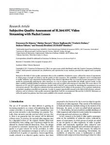
CHAPTER 2. DATA FOR URBAN ENERGY MODELLING
Figure 2.2 – Example of cadastral data, including building footprints as well as streets and other constructions.
Finally, access to most of this data tends to be restricted for privacy or marketing reasons; and when it is provided, it is often under the proviso that a confidentiality agreement is signed, thus limiting the possible uses and/or publication of the data. Close collaboration with a municipality can thus yield advantages for the collection of data.
2.2.1
Cadaster and geomatic data
Originally used for land ownership evaluation and taxation, cadasters were created in numerous countries around the world. The Cadastral Template website (PCGIAP, 2012) gathers worldwide cadastral system’s descriptions, showing how the original cadastral surveys evolved into the collection of a larger amount of land related data (Figure 2.2). Numerous cadasters nowadays include individual buildings’ footprint, and sometimes more building-related information such as addresses, ownership or construction period. Cadastral data thus offer a valuable basis for building and urban area modelling, as well as for urban energy flow map representations. The Swiss cadastre is managed individually by each municipality (although a subset of the cadastral data is gathered at the federal level by the Federal Office of Topography swisstopo) and uses the Swiss coordinates reference system. It legally has to contain the buildings’ footprints for land use information, and also contains addresses. It actually defines built surfaces, including buildings, shelters, garages and various objects with a varying relevance to energy use modelling. The identified footprint of a building might thus not distinguish between the four-storied building and the adjacent ground floor-only parking, or between the various parts of a large construction (see Figure 2.3). Even with a careful selection of building objects, it remains a coarse source for building energy demand simulation, but it is arguably the most reliable source for large scale urban simulation. 14
2.2. ENERGY-RELATED DATA SOURCES
(a)
(b)
Figure 2.3 – Examples of building footprints unfit for the creation of a 2.5D (flat roof extrusions) thermal model. (a) The right part of the footprint actually corresponds to the one floor garage that can be seen on the right of the photo. (b) The building represented by the footprint is composed of multiple parts with varying heights, ranging from 1 to 11 levels.
Other geomatic data of interest might also exist, whether included in the cadaster or not, such as: Digital terrain and surface model (DTM/DSM, Figure 2.4) The detailed altitude of the ground and the land cover is typically obtained through airborne laser based measurements (e.g. LIDAR technology), on a grid of a few meters to 10 cm sides. Orthophotos Broadly available through map services such as Google Maps (maps. google.com), airborne photographs are reprojected to match a specific coordinate system. Local administration are likely to possess orthophotos in the local projection system, with a sufficient definition to distinguish buildings and possibly their use or other useful information, such as the existence of solar panels. Subterranean and other maps Can provide information about the potential of local renewable energy sources. 15
CHAPTER 2. DATA FOR URBAN ENERGY MODELLING
(a)
(b)
(c) Figure 2.4 – Color-based representations of (a) a digital terrain model, (b) a digital surface model and (c) their difference, representing the height of built and vegetal coverage.
Energy networks infrastructure This often confidential data owned by the energy providing companies can also be available to the municipalities.
2.2.2
Building registers
Comprehensive building registers are less common than cadasters. Numerous countries have registers covering mainly historical buildings for conservation purposes.1 As the cadaster and the population census offer the possibility to handle basic building or housing information, more specific census are not always performed. However, some countries undertake such census, mainly for statistical purposes, collecting data such as the building’s construction period, allocation, owner, treated floor area, number of floors, number of dwellings or heating system. For instance, Turkey performed such a census of a large part of its real estate in the year 2000, to obtain a picture of the “quality and quantity of buildings” (Turkish building census, 2001). In Norway, the building statistics is updated at least yearly, with the purpose to “measure the developments in building activities for all types of buildings”.2 See for instance the French and English historical buildings registers on http://www.culture.gouv. fr/culture/inventai/patrimoine and http://www.english-heritage.org.uk/list. 2 http://www.ssb.no/en/bygg-bolig-og-eiendom/statistikker/byggeareal 1
16
2.2. ENERGY-RELATED DATA SOURCES
Table 2.1 – Main data of the Swiss register of buildings (RegBL) Feature National building id (egid) Address Geographical coordinates Building category Construction year Construction period Footprint surface Number of stories Heating system Heating energy carrier DHW energy carrier
Status Compulsory (always present) Compulsory (always present) Compulsory Compulsory (always present) Optional Compulsory Optional Compulsory Optional Optional Optional
In Switzerland, the register of building (RegBL, 2012) identifies all residential buildings at the national level. It stores a short description of each, based on the varying quality data that the municipalities must supply. Non-residential buildings might be included if the data is provided. This register contains some compulsory information (construction period, kind of building and of use, address) and a quite large amount of optional material: the geographical location, surface area, number of floors, construction year, renovation year or period, and possibly the type of energy system for space heating, the energy carrier used for space heating and for domestic hot water (DHW), and a boolean indicating whether there is a hot water production system. This apparently very valuable information source, largely populated based on the year 2000 census, actually reveals its limit regarding the non-compulsory attributes: energy system data is often available but almost never up-to-date, the coordinates might be absent or inaccurate, and the definition of the number of levels is not always adapted to estimate the height of the building. Nevertheless, this important data source is easily obtainable for research activities with a confidentiality agreement and provides a very valuable basis when studying build areas.
2.2.3
Inhabitant census
Much more common worldwide, the inhabitants’ census usually contain data regarding people and households (UN, 2006). It can provide interesting data for building energy demand modelling, such as the number of building occupants or the treated floor area. In Switzerland, the new census is not performed at the national level anymore; instead the Federal Statistical Office (FSO) collects the necessary data from the municipalities.3 The requirements of the federal census nevertheless ensures the collection of the same data in the same format everywhere. The census however contains sensitive data (age, nationality, religion) and is thus much less easily accessed for energy simulation purposes (but is of comparatively higher quality). More information is available on the FSO’s website: http://www.bfs.admin.ch/bfs/portal/en/ index/news/02.html 3
17
CHAPTER 2. DATA FOR URBAN ENERGY MODELLING
2.2.4
Energy providers data
Considering urban energy use, a large amount of data is obviously collected by electricity, gas, fuel oil or heat providers for invoicing purposes. This data is sensitive both for privacy and business value reasons, and thus usually difficult to obtain. A close collaboration with energy providers may grant access to this data, provided that a confidentiality agreement is signed, limiting publication options. In Switzerland, the energy providers of electricity and other network energies are usually the municipalities or owned by them. Whereas this delivered energy use data is sometimes considered as the Holy Grail by urban energy modellers, allowing for verifications or simply as the direct source for statistical analysis, its use at a disaggregated level might prove more complicated than expected. For instance, gas can be used for cooking, domestic hot water and/or space heating, with various efficiencies, while a single invoice can possibly concern several buildings (although it is attributed to one metering — or billing — address). If the precision of this data source can be considered as high, its exact attribution remains subject to interpretation. Through the quantity of energy used in one form or another, some guesses can also be made regarding the energy system used for space heating, domestic hot water or cooling. Although default assumptions are necessary, this proved to be the most reliable information to define the energy conversion systems available in buildings in our case. Indeed, the main other source on this subject in Switzerland is the non-compulsory attributes of the buildings’ register, which proved to be often incomplete and untrustworthy. Finally, energy providers are usually the only entities to know the energy networks, their efficiencies and the origin of the energy transported by them, and more generally the energy sources provided. Studying the energy flows of an urban zone without the energy providers’ collaboration thus limits greatly the detail and accuracy of the supply side modelling.
2.2.5
Meteorological data
The thermal simulation of building’s space heating and cooling demands also requires meteorological data. The meteonorm software (meteonorm.com) collects, analyses and extrapolates meteorological data in order to provide typical yearly weather data sets for any location worldwide. The hourly values necessary for building simulation that can thus be obtained include air temperature, direct and diffuse irradiation, precipitation, nebulosity, relative humidity, wind direction and wind speed. In order to compare real energy use measurement to simulated values, the real data for a specific year is needed. In Switzerland, the Federal Office of Climatology and Meteorology collects and makes available a large amount of data measured in meteorological stations around the country for a long time, most of them on an hourly basis (www.meteoswiss.ch). 18
2.2. ENERGY-RELATED DATA SOURCES
2.2.6
Energy sources
The Swiss Federal Office of Constructions and Logistics publishes a catalog (KBOB, 2009) of recommendations regarding data for energy use prediction and assessments. This catalog is based on the much larger EcoInvent database (EcoInvent, 2013), a database of “consistent and transparent life cycle inventory” which estimates the energy used to produce a broad range of material, objects or energy in various forms. The KBOB contains environmental data for a range of common energy sources, describing the impact of a unit of delivered energy in terms of primary energy used to produce it, GHG emissions associated and the share of renewable primary energy used. Documented resources include for instance oil, gas, wood log, and already transformed sources such as nuclear electricity, PV electricity, incineration electricity, average mix of distributed electricity in Switzerland, heat (on DHN) from gas plant, heat from incineration, locally used heat from solar thermal panels, etc. In a similar way, the embodied energy of construction materials is also documented, as well as energy used in its transportation.
2.2.7
Case-study dedicated surveys
For a large range of data, there remains the possibility to perform a survey in order to obtain missing data. Visual surveys of buildings’ façades can provide estimates of buildings’ age, allocation, glazed ratios of walls, etc., and possibly locate photovoltaic or thermal solar panels. Less accessible data would necessitate the inhabitants’ or owners’ cooperation (energy system installed, heating and cooling temperature set points, consumption values, etc.) or are simply not easily accessible (envelope infiltration rate, detailed construction properties). The limiting factor regarding such surveys are obviously related to time and money constraints, in contrast with the model’s use and longevity.
2.2.8
Other possible sources
Depending on the focus of the study and the local administration and organisations, other useful data sources might be available. Less usual but potentially useful data sources range from chimney sweep data (which in some places contains the kind and possibly the efficiency of individual heating systems) to official firm census (containing usually sensitive data about all firms in a district such as the kind of activity and the number of employes), through natural resource maps or construction policy. Perhaps more important, although less identifiable, some local civil servants and energy provider employees are likely to possess knowledge about the buildings and their energy supply. Accessing this knowledge or its ability to detect glaring errors does require some form of collaboration, but most importantly, it requires a clear and direct access to the data, for instance as map representations. 19
CHAPTER 2. DATA FOR URBAN ENERGY MODELLING
2.3
Availability, quality and disparity
The last section evidenced the numerous possibly useful data sources for urban energy flow modelling on a per-building basis. However, the main difficulties lie in the collection, sanitation and harmonisation of data from various sources, in the setting up of its actual management and in its updating.
2.3.1
Data collection
The registers discussed above are often scattered amongst various departments, and even when the data is freely available for research purposes, the acquisition processes are varying and not straightforward. Moreover, while the cadaster, building register and census may be exhaustive, the other data sources discussed are likely to not fully cover the area of interest. Most urban energy modelling activity thus primarily use the official records, although these are usually not particularly concerned with energy, and do not intend to provide precise data in this domain. In Switzerland, the national records are also the most accessible, as a law from 2008 (LGéo) requires that of a range of geodata is made available for both public and private use. The new portal map.geo.admin.ch thus grants a unified access to visualise public geodata, such as maps and orthophotos from the swisstopo office, and a subset of the building register’s data. The website does not actually centralise all the data and does not offer download functionalities, but it provides links to order complete datasets from the corresponding federal entity. The level of detail of data available at the level of municipalities might however be higher, for instance for cadastral data. Depending on the case study, many of the third party or less accessible data sources will simply not be considered, as their value for modelling does not seem to be worth the necessary time investment. Online access to compatible third-party databases, although the subject of research as part of the “semantic web”, is still far from being a common reality in the domains explored here, where most of the data is not public. Even when the acquisition of some raw data is rapid, the difficulty can be to obtain information about the data, its definition and its units. One usually has little influence over the format of the data provided by third-party sources, and must adapt to whatever can be obtained. Thus the usability and actual use of the numerous data sources discussed above is disappointingly low in practise.
2.3.2
Quality and updating
It has been stated that some official data, although not exactly adapted for our purpose, is very precise and complete (mainly cadaster and census data). Still, for most of the data gathered in an informal context, the confidence level is quite low, whether it lacks an adapted formal definition (independent sources such as energy providers) or because an optional status makes its collection and update uncertain. It must be noted that the knowledge about the quality of data is often acquired through the use of the data, and not automatically transferred with it. Estimating be20
2.3. AVAILABILITY, QUALITY AND DISPARITY
Figure 2.5 – Example of incompatible data units: two cadaster footprints, seven addresses (green points), five register of building entries (yellow points), three gas consumption measurements (the largest must actually be attributed to both buildings) and one electricity use measurement (also concerning both buildings).
forehand what data can be trusted is thus difficult, and choosing which source to trust when redundant information do no agree is sometimes random. Managing this data, it is likely that obvious corrections will promptly be made, without history tracking or feedback to the original source. To clarify the status of data seems to us of paramount necessity, and the possibility to tag data with information about its source and estimated quality will be discussed in the next chapter. Although a high quality and compatibility of data is still the exception, third-party registers are likely to be regularly updated, and the current tendency is towards further improvement of registers in the future. These data sources are thus of great interest for the research and development of data models, which suffer from lack of longevity. The data used for research and simulation should be based on these third-party registers in such a way that the models are as straightforward to create as possible and can be easily updated when the third-party sources are completed, corrected or updated. This will also be one of the objectives of the next chapter.
2.3.3
Disparity and incompatibilities
The combination of data from various sources generates an other difficulty: most sources are not used or managed together and are consequently incompatible. Conflicting values (e.g., the buildings register records that a building is heated with a boiler, but the energy provider gives a district heating consumption) can be solved based on knowledge about the relative quality of the sources, if any. Otherwise, random guesses are likely to be made. A more tricky point is the mismatch between the objects in different sources. One cadastre building may correspond to several entries in the buildings’ register or in consumption data from energy providers (Figure 2.5). The decisive data source is likely 21
CHAPTER 2. DATA FOR URBAN ENERGY MODELLING
Figure 2.6 – Example of a cadaster footprint corresponding to two address points on different streets. In this particular case, one address was recorded in the register of building, whilst the other was used to identify consumption data.
to be chosen without pattern, unless a preliminary choice is made regarding which data source defines the entities to be modelled. Finally, the mere correspondence of data in two different sources might prove difficult to establish; just as there is no common data entity, there is not always a common identifier. Most data sources use addresses, but the latter might be written in various forms (making simple automatic match inefficient), and one building can have several of them, not necessarily on the same street (Figure 2.6). Some sources rely on object numbers, these identifiers being sometimes local and not shared with other data sources (e.g. client number for energy consumption data). Spatial localisation is increasingly used (for instance on platforms such as map.geo. admin.ch) and is sometimes the only shared information, for instance between the cadaster’s various layers (such as addresses, building entities and DTM or DSM). The use of geolocalisation to combine datasets requires dedicated GIS software. The spatial matching of sources is a usually efficient data combination method, but can be complicated by the use of different coordinate systems, or by slight imprecisions in the positions of objects.
2.3.4
Temporality
Although an obvious remark, the fact that our object of modelling is continuously changing is another aspect that is often dismissed in urban energy simulation. The data sources describe their domain of interest at a time corresponding to their last update in the best case, or at mixed times of update in the worst. Using the same means as for other inconsistencies, sources describing the same area at different periods can be combined to obtain a model. However, the temporal evolution of the situation might also be of interest. Energy use measurements refer to a specific period, and to the buildings and energy conversion systems existing at that period. Annual energy use monitored data is sometimes available for several years, allowing for evolution studies. The changes in energy use must however be considered together with the changes in the energy situation of the concerned urban area. Whereas simulation scenarios is a common subject of study, the tracking of real 22
2.4. DATA MANAGEMENT AND STORAGE
changes’ effects should not be overlooked. Modelling this temporal dimension is thus another challenge, that will be discussed in Chapter 3.
2.3.5
The role of default data
The usually available data is obviously not detailed enough for micro-simulation, which calls for the use of adapted default data to complete the picture. However, the definition of the default values and the manner they are used rise numerous questions. Firstly, where obtaining real data is difficult (construction details such as wall composition, energy conversion system efficiencies, etc.), establishing reasonable default values is a challenge, and dedicated studies can be rare. Whereas professionals can suggest orders of magnitude and simulation can explore their adequacy, exact measurements are often not available. This subject will be discussed in more detail in Section 3.4. Secondly, where data is available but incomplete, default data can either be used systematically, or in combination with real values. The first option is simpler, as the limit between input model data, default data and simulated values is thus well defined. It is nevertheless not appropriate when trying to represent reality as faithfully as possible: definitely fixing those default would considerably limit the advantages of the microsimulation approach. The second option, completing existing data with default values, raises the question of traceability, already mentioned about corrections and hypotheses: it is necessary to know what data is real, and what part is default. On the other hand, it places no limit to the improvement of the model should more data become available, and ensures that the default values are visible. An extended and systematic use of default data would also bring micro-simulation closer to a statistical approach. The use of micro-simulation with default values only where no data is available offers two decisive advantages: the possibility to make the model more precise, and the possibility to simulate the impact of specific and detailed parameters on the overall energy efficiency.
2.4
Data management and storage
Dealing with the difficulties discussed above leads to the question of how to avoid worsening the data reliability and repeating the same mistakes. The data sources are usually obtained in the form of various format files (.xls, .txt, .shp, .dwg, .csv, ...). Ironically, the antithesis of sustainable data management is common practise: using these source files, data will often be organised in the form of a simulation’s input file. This unstructured process, for which modifications cannot be traced, complicates the access and update of the data, and thus compromises the durability and reusability of the model. Obviously, a structured data management is necessary to improve the quality and utility of the data. To this end, this section proposes an overview of available data management tools and analyses their fitness for the management of urban energy models data. 23
CHAPTER 2. DATA FOR URBAN ENERGY MODELLING
2.4.1
Geographical Information Systems (GIS)
Considering geographical data, Geographical Information Systems (GIS) such as ArcGIS and Manifold (both commercial) have successfully spread, amongst other for numerical cadaster management. They provide a visual and user-friendly way to access and use data through maps, with a strong emphasis on geographical data, analysis and presentation. They can thus store and manage (mostly 2D) geographical data, and properties associated to the geographical entities. Apart from their graphical interfaces and visualisation tools, a large part of their functionalities are similar to those of databases (discussed in Section 2.4.2). These programs can also be used in combination with a database management system for the storage of data. However, they impose strong limitations in terms of data model compatibility (for instance, all data object must be spatial and have a geometry). For commercial solutions, the accessibility through third party software is limited. GIS can also be used to a certain extent to access the contents of third-party databases, but with limited compatibility and editing functionalities. The use of a GIS thus depends on the users’ needs and preferences, but their limitations can be problematic in a research and development context, or when dealing with complex structure data.
2.4.2
Database management solutions (DBMS)
Database management systems (DBMS) have been around for almost fifty years, and are now extensively used to store and manage data. Most currently available DBMS provide more extensive functionalities, with PostgreSQL (open-source) and Oracle (commercial) being amongst the most advanced spatial databases. Almost all DBMS follow the SQL (Structured Query Language) standards for the input and retrieval of data, provide application programming interfaces (API) to access the database through self-made programs and offer server functionalities for remote access. What database management solution gain in flexibility, they perhaps loose in simplicity and user-friendliness: without map representations, the data must be accessed mainly through SQL queries. Using SQL, the data needed for simulation can be retrieved with precise queries either to text files, by a small program creating a specific input file, or by the simulation program itself, if it is adapted to use the database, for input as well as output. The database can also be stored on a server to be accessed and modified remotely by multiple users working on the same project. Without a “geometry-and-attribute” structure imposed, it is necessary to define the detailed structure of the required data model. Most DBMS handle relational models, based on tables (or relations) containing lines (or tuples) identified by keys. Relations and references between tables can be defined, with constraints guarantying the coherence of the data. 24
2.4. DATA MANAGEMENT AND STORAGE
2.4.3
Spatial DBMS
Advanced spatial DBMS started to emerge at the beginning of the 1990’s to meet the demand for geographical data storage (Güting, 1994), leading to the definition of the standard Simple Feature by the Open Geospatial Consortium (www.opengeospatial. org). This standard defines new data types (points, linestrings, polygons, etc.) and functions to create, access, manipulate or combine them. Spatial -DBMS can thus manage 2D or 3D geometries, offering the same spatial functionalities as GIS (distance between objects, overlap, etc.). Most leading DBMS now offer these standard spatial types and functions or have implemented them as a complementary spatial module, and have optimised the methods to handle the queries on them. For PostgreSQL, the PostGIS module defines the necessary data types and functions. Whereas the DBMS themselves do not usually offer data visualisation functionalities, some open-source softwares such as QuantumGIS can fulfill this role.
2.4.4
Temporal DBMS
Temporality is another domain of current research: multiple applications require the temporal dimension to be taken into account. If the storage of time or date data types has long since been common, the coherent handling of the continuous nature of time remains the focus of development effort (Jensen and Snodgrass, 2002). An increasingly common approach is that of bi-temporal databases, which store for each entry its valid time, i.e. the time period during which the data is valid in the modelled reality, and its transaction time, i.e. the time period when the data is valid in the database. Support for these temporalities is still limited; in particular, it is currently extremely complicated to write constraints related to the temporal validity of data.4 Most DBMS do not offer a complete temporal data management solution (with the exception of Oracle’s “Workspace Manager”). However, basic temporal functionalities of DBMS can be used to create a structure to manage the temporal aspect of the reality modelled. PostgreSQL for example offers an extension called “Timetravel” which can be used to keep the original version of the data when it is modified. It does so by adding to each table additional fields to save the transaction time, i.e. to define the period of time when the data was valid in the database, so that the state of the database at any point in time can be retrieved through a filter on these fields, without saving new versions of a file each time it is modified. A versioning control mechanism — saving the original version of the data and keeping track of the successive modifications to be able to reconstruct any version — is out of the scope of standard DBMS and thus usually not implemented. However, such a system is used for the versioning functionality of ArcGIS5 , and could In temporal databases, the same object can be described for various periods of time, and thus correspond to several entries. However, a typical constraint is that there should not exist two versions of the same object at the same valid time and at the same transaction time. This is currently difficult to express in constraints, with the exception of the new exclusion constraints in PostgreSQL 9.0. Even with this advance, the verification of references’ validity becomes quickly perilous. (Date et al., 2003) 5 In ArcEditor and ArcInfo, using ArcSDE geodatabases 4
25
CHAPTER 2. DATA FOR URBAN ENERGY MODELLING
also be built again on a database, although it might greatly limit the efficiency of SQL queries. Finally, research is also exploring the unification of time and geography in spatiotemporal databases (Pelekis et al., 2004). Nevertheless, the full range of these functions has yet to be implemented in most available DBMS.
2.4.5
Database for urban energy simulation
In the present doctoral thesis, we considered that an adequate data management solution must: • Allow for the structured storage of all the kinds of data considered, which is actually a constraint when dealing with geographical, temporal or raster data. • Support the quantity of data involved and possibly much more, placing no limits on the size of the models. • Provide convenient ways to import data and export it for modelling tools. • Allow for automatic retrieval by means of third party programs. • Allow the user to track modifications or to create a mechanism to do so. • Allow for several people to work on the same data through a server system. This naturally motivates the use of a well-structured database in a DBMS. The tendency not to use a formal database for short-term energy modelling projects is arguably related to a lack of knowledge about DBMS and to the investment in time it requires. However, the numerous advantages of databases mentioned above clearly compensate for the workload of creating the database; in particular if the same kind of data is used regularly for similar studies. This does however require that a complete data model be defined for the domain of interest, usually in the form of a relational model. It is the subject of the next chapter.
2.5
Limitations and opportunities
This chapter explored the role of data in urban energy flow simulation. We evidenced that data availability and management are essential components of the simulation process and must not be overlook. After a brief survey of the usual approaches of data in urban energy modelling, the main type of data sources that can be used in our domain were reviewed. The related difficulties discussed in Section 2.3 appear in any real-world study. The handling of these difficulties usually includes guesses, random choices and renunciation to secondary or incomplete sources. The process of creating an adequate input model for practical studies obviously remains a side question during the development or validation of a simulation tool. When it comes to reality-based modelling and simulation, the quality and representativeness of the input model must become a primary concern. Indeed, in order to inform about the energy use of an urban area and to explore possible evolutions and alternatives, a large 26
2.5. LIMITATIONS AND OPPORTUNITIES
amount of reliable input data is necessary. Obviously, a fully informed and correct model is not accessible, and should not be the objective. However, there are some flaws inherent to the construction of the model that can be improved or avoided entirely. It possibly requires several changes in the modelling paradigm, the first being a greater focus on data and data management. The data management solution playing an important role in the quality and durability of the data model, current functionalities of geographical information systems (GIS) and database management solution (DBMS) were also presented. The greater flexibility of DBMS promote their use when the structure of data is not purely spatial, and when compatibility with third-party software is required. However, the advantages of a visual access to the data through map representations must not be overlook: inaccessible data cannot be understood, verified or updated.
2.5.1
Model longevity
The quality of an urban zone model is strongly connected with its longevity. At some point, improving the quality of a detailed data model of an urban zone is only feasible if its longevity and thus usability is also increased. On the other hand, whereas a specific study can rely on a dedicated input model, urban energy management requires a longer term approach. A model intended to perform a predefined study in a finite time is unlikely to be usable may any new question arise after some time. Moreover, studying the evolution of the energy use also requires an enduring model. There are thus several reasons to aim for longevity together with quality. Obviously, the goal of research cannot be to maintain databases on the long term, but developing a framework to do so is a relevant purpose. The short term benefits for modellers are numerous and worthwhile. Moreover, if a model is actually useful to municipalities or energy providers, it can be used, improved and updated by them. The existence of such models is again beneficial to modellers, as it greatly facilitate the performance of new studies.
2.5.2
From data to information
The organisation of data into a structured model actually corresponds to the first step in the process of transforming raw data into useful information. As such, a high quality input model created for a specific simulation task might be in practise as valuable as the output of the simulation. However, exploiting this value might require a change of paradigm regarding data: instead of considering simulation results as the primary objective, simulation can be seen as a tool to complete an urban energy flow model. A general model, whether it is explicit or not, is always the actual backbone to interpret data, and thus create information. As thus, we postulate that much can be gained by considering explicitly the model as the main focus, while simulation is used to complete or detail the model. Figure 2.7 represent such a structure, proposing an alternative to the process described earlier by Figure 2.1. 27
CHAPTER 2. DATA FOR URBAN ENERGY MODELLING
Simulation software
.shp Cadastral map
Output treatment
.csv Climate data .xls Buildings’ register .xyz DTM / DSM ...
Simulation software
Input preparation
Input preparation
Output treatment
Simulation software
Data import
Enduring model / Appropriate data storage system
Input preparation
Results reading
Results reading
Figure 2.7 – Data for urban energy simulation: organised management of data proposed in this work. The simulation input creation and output treatment based on an enduring data model can be automated, thus multiplying the benefits of the necessary work on data to create the model.
Creating a detailed model for urban energy use management is doubtlessly an ambitious and time-consuming task. Nevertheless, if it is addressed efficiently, the model might be able to take advantage of complementary simulation programs, and may in principle be transferred to municipalities to maintain and perform studies of their own. Thus the greater need in data and time of such a model can be balanced by its longevity and its various uses.
2.5.3
A blurred limit between data and simulation results
Given our objective to model urban energy flows using multiple simulation models together with real measurements, the ordinary differentiation of data between input and output becomes inappropriate. On taking a closer look however, even when considering a unique simulation tool this apparently clear distinction is not that obvious: the use of default values to create an input model is already a reproduction of a known pattern to obtain results, which approach our definition of simulation (Section 1.2). Regarding the combined use of monitored data and energy use simulation, how the simulation of the energy flows can be performed without ignoring data that corresponds to a simulation’s output will be the subject of Chapters 4 and 6. In the meanwhile, this also means that the data structure must be adapted not only to differentiate between original data, default values and simulation results, but also that it needs, for instance for energy quantities, to handle both monitored and simulated values. 28
2.5. LIMITATIONS AND OPPORTUNITIES
Table 2.2 – Summary of problems regarding data evidenced in Section 2.3 Cause
Result
Direct creation of simulation input file
Dropping of original and non-relevant data, very limited reuse possibilities for other studies
Rigid model
Dropping incomplete data in favour of default values
No tracking of data
Undistinguishable mix of reliable data, uncertain data, guesses and default values
File-based solution
Limited accessibility; difficulty to update and improve data; difficult or impossible access by third party
Unstructured study of multiple years and scenarios
Copy of the model, further improvements either limited to last version, or to be performed in numerous files; difficult comparison with previous situation
Blurred limit between original data and simulation results
No simple input / output boundary
2.5.4
Directions for the data structure of our framework
The next chapter is dedicated to the construction of a conceptual data model and a data management structure for urban energy flow. The creation of a structured data model adds a step in the urban energy simulation process, between the data collection and the input preparation for a simulation model. The goal of this intermediate stage is to improve the model’s longevity and usefulness, by providing an opportunity to tackle the problems summarised in Table 2.2, providing support or solutions wherever possible. Whereas the data management method and conceptual model cannot create the data quality, their careful choice and set up will mitigate some of the difficulties met during the data preparation and thus help improve the quality and longevity of the model itself.
29
Chapter 3
Conceptual data model (CDM) Starting from the state-of-the-art and the shortcomings related to data management for urban energy simulation, we intend to develop a more sustainable and holistic approach for urban energy flow simulation. In the introduction we emphasised the necessity to consider the following objectives: . Manage all the relevant data for urban energy flow micro-simulation. . Gain time in the creation of the model. . Maximise the utilisation of available data. . Increase the model’s longevity by simplifying updates. . Keep track of data model modifications and / or simulation scenarios. The next section will complete or detail this with a whole set of objectives regarding simulation goals, tools and the data considerations of Chapter 2. These objectives form a background for the design of the conceptual data model (CDM) described in Section 3.2 and the features added in Section 3.3 to create an actual simulation framework. Section 3.4 presents the numerous default values involved in our simulations, while Section 3.5 describes the implementation of the conceptual model as a relational model in PostgreSQL.
3.1
A bridging role
We discussed in the last chapter that a simulation tool input file format is usually not an appropriate data structure for urban energy flow modelling. It was also observed that the data available from third parties is rarely dedicated to this subject, and at the least incomplete in this domain. However, neither of this data realities can be ignored if a useful data model is to be developed. In this sense, the conceptual data model can be seen as a bridge between the studied reality (an urban energy system), the available data describing this reality, and the simulation tools with their very specific model of the reality (Figure 3.1). 31
CHAPTER 3. CONCEPTUAL DATA MODEL (CDM)
Available data and data sources
Existing simulation tool input data Conceptual model
Interests / simulation goals
Figure 3.1 – The conceptual data model seen as a bridge between the studied reality, the available data describing this reality, and the simulation tools with their very specific model of the reality.
The CDM is thus at the intersection of these three worlds. It intends to decrease the difficulties linked with the data preparation discussed in the last chapter, but also to provide the necessary data to simulate the buildings’ energy demands, their supply and the energy systems as a whole. The simulation objectives determine up to some point what needs to be modelled and at what detail, but can only be met based on the available data. Even if some simulation tools to be used at first with this simulation framework are already defined, the data model must remain as independent of them as possible. It is more appropriate to keep the data in a format close to the original one rather than in a specific simulation tool’s input format; using a well-defined conceptual model to store the data, the preparation of specific input files is a task that can easily be automated in a dedicated module. Furthermore, no potentially useful data is to be dropped because the current simulation tool does not use it, when it could be used by an other simulation tool to produce other or more precise results. There are many subjects related to urban energy flows that are not considered in this work for lack of time, such as hourly load profile study or distribution network detailed modeling and simulation. However, these possible future developments are not simply ignored in the creation of the conceptual model. The conceptual model and its implementation are intended to be easily adapted or extended to permit a more thorough treatment of these subjects. This can be summarised in the following objective, developed in Section 3.1.3: . Model the urban energy picture in a coherent way, compatible with the various kinds of simulation tools that are to be used but not necessarily shaped by them. (The simulation tools that will be used in this work are described in Section 3.1.3) 32
3.1. A BRIDGING ROLE
3.1.1
Modelling role and objectives
Our data model is primarily dedicated to our simulation objectives: namely, simulating the urban energy flow at the disaggregation level of the building. In more detail, specific goals include: 1. Model existing neighbourhoods and buildings for spatially specific results. 2. Distinguish between the main energy services in buildings (we consider here space heating, space cooling, domestic hot water production and electricity services, but these could be detailed). 3. Model explicitly situations where multiple energy conversion systems (ECS) providing the same service (for instance solar thermal panels and gas boiler producing DHW). 4. Model explicitly ECS providing several services and/or several buildings. 5. Handle distribution networks (heat, gas, electricity) and the mixed origin of the energy they deliver. 6. Provide access to useful energy, delivered energy and primary energy use values, as well as green house gases (GHG) emissions and renewable energy use, per building, urban zone, energy service or energy carrier type. 7. Integrate available energy use measurements to improve the model. 8. Provide monitoring of yearly energy use evolution. 9. Support the study of scenarios defined as modifications of the base case model (which represents the real status of an urban zone). 10. Use maps as the primary interface for interaction with data and results representation. The first item excludes a fully statistical or aggregation approach; whereas uniform default values might be necessary, any specific information available must be used to represent the urban zone as it is. Together with the second item, it necessitates the consideration of building objects, to which four energy demand objects (one per service) will be attributed. Item 10 requires a geometrical representation of the building objects; the data available and the simulation approach for energy demand simulation will define most of the other parameters needed. However, the goals of items 3 and 4 preclude a model based only on buildings and their simplified energy supply: it must be possible to assign any number of energy conversion systems (ECS) to the provision of each service in each building. Conversely, it must be possible to attribute the energy production of one ECS to several building’s demands, which is also required to satisfy item 7. This leads to the choice of a system approach with a graph structure, which will be discussed below in Section 3.2.1. Item 5 and 6 advocate the addition of network and source objects in the graph structure. Thus energy quantity data need to be associated not only with building objects, but also with the other energy nodes introduced here, or to a specific flow between two of them. 33
CHAPTER 3. CONCEPTUAL DATA MODEL (CDM)
Networks
Sources
Energy conversion systems
Building «sink» nodes
Building B1 B1 electricity need
electricity Hydropower electricity electricity
Nuclear power
gas Natural gas
Electricity meter
Combined heat and power plant
Local grid
electricity
electricity
heat Elec boiler heat
Solar thermal panels
electricity
heat
heat
B1 space heating need B1 domestic hot water need Building B2
DHN
heat
Heat exchanger
heat
B1 space heating need
Figure 3.2 – Example of a partial energy system model, showing the energy supply of two buildings.
Item 8 states that we are interested in the evolution of the energy use, at first on a yearly basis. This means that energy quantity values cannot be associated only to an energy node, they must also refer to a time span, here fixed at a year. The energy quantity data will thus be stored in annual energy flow objects in the model. Moreover, the evolution of energy consumption is only interesting when correlated with the evolution of the buildings and their energy supply chain. The temporal evolution of these objects is thus also of interest. Item 9 raises an other fundamental point, requiring the storage not only of a representation of the existing urban energy picture (or base case model ), but also of alternative attribute values or objects, defining scenario models. In terms of data model, this translate into the following requirements: . Model the building, ECS, network and source as independently energy nodes objects, together with their interconnections (with an energy flow meaning, see Figure 3.2). . Represent annual energy flow objects attached to the energy nodes and attributed to a specific year and scenario. . Record the temporal evolution of the whole urban energy system (Figure 3.3). . Store variations of the energy system data as scenarios (Figure 3.3).
3.1.2
Influence of the available data sources
As a matter of fact, the data sources discussed in the last chapter determine what data can be relied upon and what cannot be expected. As the most covering sources are the cadaster and the Swiss buildings’ register (RegBL), our model is based on the objects and attributes that are consistently found there: buildings with their footprint, period of 34
3.1. A BRIDGING ROLE
1912 1913
...
...
1987 1988
...
...
2005 2006
Building B1 (built in 1913)
...
...
2013 2014
...
B1 (windows changed in 2005) Base case
Oil boiler (installed in 1987) Building B1 (built in 1913)
B1
B1 (insulated) Scenario
Oil boiler (installed in 1987) Heat pump
Figure 3.3 – Example of a temporal evolution and scenario modelling. A building built in 1913 has its windows changed in 2005, and is currently heated by an oil boiler installed in 1987. In a scenario for 2014, one might study the possibility of insulating the building and replacing the oil boiler by a heat pump. Table 3.1 – Example of data source format used in the conceptual model: period definition and codes from the RegBL (building register), used to encode the buildings’ construction period and attribute default values. Code 8011 8012 8013 8014 8015 8016 8017 8018 8019 8020 8021 8022 ...
Period Before 1919 1919 to 1945 1946 to 1960 1961 to 1970 1971 to 1980 1981 to 1985 1986 to 1990 1991 to 1995 1996 to 2000 2001 to 2005 2006 to 2010 2011 to 2015 ...
construction, height or number of storeys, address and identifier. These were decided to be the set of compulsory data. It forms an extremely rough model, but requiring more compulsory data is likely to result in the use of arbitrary default data, whereas requiring only basic building information ensures that the default values needed will be attributed according to the framework’s predefined rules and known as such. Nevertheless, the nonhousing buildings being only optionally included in the RegBL, even that rough model might necessitate some other data source or guess work. Beyond the compulsory attributes, all relevant data available in the identified sources is included in the model, even if their use is not straightforward. The standard formats and codes are kept whenever possible. For instance, the definitions and codes of the RegBL for 35
CHAPTER 3. CONCEPTUAL DATA MODEL (CDM)
the buildings construction periods are adopted, and the default values depending on the age of the building will be attributed based on these construction periods (see Table 3.1). The choice of other periods might be more relevant for the attribution of default values, such as periods based on the evolution of construction methods. However, other periods would be almost impossible to use: the RegBL is the most reliable source regarding the construction period of the buildings, but the exact construction year of the buildings is rarely available. Other data, which are relevant to our domain of study but not useful for the short term purposes, are also to be included. For instance, the RegBL contains an (optional) refurbishment date, which might correspond to any energy-efficiency driven measure or to some energy-unrelated work. Although not used currently or in this work, this possibly valuable data is included in the data model. In summary, regarding the data sources and preparation, we add the following objectives for the creation of our data model: . Impose a minimal set of compulsory data. . Provide for a flexible and structured use of default data. . Use the sources’ structure and format of data wherever possible. . Include all relevant available data. . Automate a first check of data validity (range checking and other simple rules).
3.1.3
Existing simulation tools and their data requirements
It was stated in the introduction that the goal of this work is to simulate the energy flow of urban areas using existing tools when available: CitySim to estimate the energy demand and Energy Technology models to simulate the energy conversion systems. Although our data modelling is not to be defined by these tools, their input and output formats must be taken into account. CitySim The simulation of buildings’ energy demands must be possible with any simulation tool, but is currently performed by CitySim. The urban energy use simulator CitySim (Robinson et al., 2011) was developed at EPFL based on multiple physical models coupled together. CitySim can compute an estimation of the on-site energy use for heating, cooling and lighting with an hourly time step. A radiation model first computes the irradiation incident on each surface of the scene, direct from the sun, diffuse from the sky and reflected by other surfaces. The results of this model, together with predictions of long-wave radiation exchange, are input to a thermal model. This model determines the thermal exchange through buildings’ envelopes and computes the heating and cooling energy needs to maintain predefined temperature conditions inside. Finally, ECS providing heating, cooling and electricity can also be defined. 36
3.1. A BRIDGING ROLE
As input, a complete physical description of the scene as well as climatic data are needed for the simulation. The climatic data includes hourly temperature, wind and irradiance values, together with the geographic coordinates and the definition of far field obstructions (which is used by the radiation model). The building models describe the envelope of each building (including the thermal properties of each facade, the layered composition of the walls with thermal inertia and transmittance properties, the proportions of window and the physical properties of glazing), as well as building-wise parameters such as infiltration rate, temperature set points and the presence of occupants and heat gains. Table 3.2 gives a global view of the input data required for a simulation of heating and cooling loads. Most of this information will be extrapolated from the footprint, height and age and the building, as more data is rarely available. But as the simulation uses more detailed parameters, the most influencing will be individually definable instead of using fixed default values. The building objects of our model are thus based on the coarse available data, but include more detailed parameters for which default values are provided. For time reasons, this scheme has been applied only up to some detail: some extrapolations are currently not modifiable, such as the 2.5D geometry of the envelope (based on the footprint and average height) and the internal heat gains (based on norms regarding occupancy and electricity consumption). Simulation models of energy conversion technologies For the simulation of the energy systems, existing models of the Energy Technology database of the Industrial Energy Systems Laboratory (LENI) of EPFL are used (Bolliger et al., 2009).1 The simulation models were provided together with the dedicated data model shown in Figure 3.4 by Jakob Rager of the LENI laboratory. The data regarding efficiency and other parameters of the energy conversion systems is almost inexistent, thus a default value is attributed to each parameter, and simple models mostly based on an efficiency parameters were chosen. This data model was kept more or less as such, as data sources do not influence it, and the existing representation is flexible enough to deal with any kind of technologies. Other simulation tools As stated earlier, our framework is developed around existing simulation tools, but intends to remain as independent as possible from those specific tools. It also intends to permit the more detailed simulation of any aspect of urban energy flow. At the present, the simulation of buildings’ DHW and electricity demands is an estimation based on norms of yearly need per meter square, which could be improved. Another area of interest is the spatially explicit simulation of distribution networks, instead of the consideration of a simple loss factor. District heating networks are of particular interest, as losses are We differentiate here the conceptual technologies from their materialisation in individual energy conversion systems: the same energy conversion technology model will be used to simulate numerous ECS. 1
37
CHAPTER 3. CONCEPTUAL DATA MODEL (CDM)
Table 3.2 – CitySim data requirements (for this work’s use: simple energy demand simulation only). altitude latitude longitude meridian Climate Year hourly values
id infiltration rate min and max set point temperature
temperature wind speed wind direction relative humidity nebulosity rain fall horizontal global irradiance
[°C] volume thermal bridge φ
Roof surfaces
Thermal zones
Ground surfaces
Wall surfaces
Heat gains id Wall types
38
Layers
[W/m2 ] [h−1 ]
District Buildings
[m] [˚N] [˚E] [h] [°C] [m/s] [˚] [%] [okta] [mm]
thickness conductivity heat capacity density
geometry U-value reflectance windows ratio w. U-value w. g-value w. openable ratio geometry U-value geometry wall type id reflectance windows ratio w. U-value w. g-value w. openable ratio total yearly gains year hourly profile
[m3 ] [W/K] [m] [W/(m2 ·K)] [-] [-] [W/(m2 ·K)] [-] [-] [m] [W/(m2 ·K)] [m] [-] [-] [W/(m2 ·K)] [-] [-] [Wh] [-] [m] [W/(m·K)] [J/(kg·K)] [kg/m3 ]
3.1. A BRIDGING ROLE
Technologies PK TechID TechnologyName DisplayName Description
TagsTable PK TagID PK,FK1 TechID TagName DisplayName Description SI-Unit DefaultValue DefaultValueMin DefaultValueMax
TagValue PK
TagValueID
FK1 TagID Value MinValue MaxValue Steps FK1 TechID
Figure 3.4 – LENI’s Energy Technology database extract (source: Jakob Rager).
sizeable and highly variable. This is not part of the present work, but the data structure also considers this possibility. In summary, the planned use of simulation software leads to the following objectives for the creation of our data model: . Include the detailed simulation parameters needed for energy demand simulation and energy conversion system simulation. . Define compulsory data and provide defaults for other attributes. . Keep the model as independent of the chosen simulation tools as possible. . Maintain the possibility of more detailed simulations.
3.1.4
Remarks regarding existing conceptual data models
The subject of data organisation and structuring, with goals such as information creation and data exchange improvements, has naturally been tackled by researchers in other domains, some of them being close to the urban energy domain. At the level of the building, considering in particular the construction process and the many specialists involved, the need for a common modelling language is crystallising around the acronym BIM, for Building Information Modelling (Eastman et al., 2011). Multiple BIM standards exist, such as Autodesk’s BIM, Graphisoft’s Virtual Building™or the International Alliance for Interoperability’s BuildingSMART™. The objective of BIM is to provide a unified framework for the enriched modelling of a building, at the intersection of architecture, engineering, construction and operation industries. Many tools thus make use of BIM, although Succar (2009) highlights the “need for a framework that positions BIM as an ‘integration of product and process modelling’ and not just as a disparate set of technologies and processes”. The lack of a widely accepted standard, 39
CHAPTER 3. CONCEPTUAL DATA MODEL (CDM)
together with the very high level of detail at which BIM operates and its usual focus on a single construction thus limits its relevance for our domain of modelling. Arising from the more delimited domain of 3D visual representations of buildings (and latter cities), the CityGML information model offers a standardised language for the modelling of buildings. The official website2 offers the following description: CityGML is a common information model and XML-based encoding for the representation, storage, and exchange of virtual 3D city and landscape models. CityGML provides a standard model and mechanism for describing 3D objects with respect to their geometry, topology, semantics and appearance, and defines five different levels of detail. Included are also generalization hierarchies between thematic classes, aggregations, relations between objects, and spatial properties. CityGML is highly scalable and datasets can include different urban entities supporting the general trend toward modeling not only individual buildings but also whole sites, districts, cities, regions, and countries. CityGML is an open standard based on the Geography Markup Language (GML) standard of the Open Geospatial Consortium3 . In spite of its status as a standard that makes it an important format in the domain of geospatial modeling, the interconnection of its core definition with the domain of energy is mostly limited to buildings, and (currently) to a largely non-physical representation of these (for instance, the precise location of surfaces can be defined, but their thermal properties are not included). It thus cannot be considered as a readily usable basis for an urban energy conceptual model. The CityGML standard however offer extension possibilities through Application Domain Extensions (ADE); some are currently under development such as a SolarADE or a UtilityNetworkADE4 . The development of a compatible conceptual model of urban energy would be a valuable feature and could become the basis for a standard format. However, the limited compatibility of the existing CityGML features with the subject of this work, together with the intend to exploit the advantages of database management systems (instead of XML-formatted text file), lead to the choice not to use the CityGML format for the definition of our conceptual data model. An adaptation to this format, or at least an import / export compatibility represent a worthwhile possible future development. To our knowledge, no urban other energy modelling standard exists, which would encompass our domain of interest. The next section will thus introduced a new conceptual model of the urban energy system.
3.2
Conceptual data model structure
The objectives identified in the last section shaped the conceptual data model described here. Some of them led to features that are rarely implemented, while no model known to us proposes all of them together. 2
http://www.citygml.org http://www.opengeospatial.org/ 4 http://www.citygmlwiki.org/index.php/CityGML-ADEs, last checked 01.02.2014 3
40
3.2. CONCEPTUAL DATA MODEL STRUCTURE
In particular, energy flow models often lack the capacity to represent correctly the complexity of the energy system, adopting simplifications or approximations that are only valid for a specific domain or study. For instance, a building’s hot water might be provided by solar thermal panels and completed by a natural gas boiler, which also provides space heating. Depending on the subject of interest, either the space heating or DHW demand might be ignored, as might the solar thermal panels or the boiler. However, in order to keep insight on the global use and origin of energy, this situation can clearly not be handled in a “one building”-“one energy system”-“one energy service” approach. Furthermore, the intent to consider monitored data highlights its natural attribution to ECS instead of buildings: a gas consumption usually corresponds to a gas boiler, whether this boiler provides only one energy service in one building or several services in a group of buildings. This led us to a system approach, for both our conceptual model of the energy system (CDM) and our energy flow simulation approach. Specific aspects of different energy elements can thus be simulated with various existing specialised simulation tools: building’s energy demand are simulated independently of energy conversion systems or distribution networks. The simulation methods discussed in Chapters 4 and 6 then consists in exploiting specific simulation tools in an integrated way to obtain a picture of the energy flow on the whole energy system. The necessity to correctly model real urban energy flow thus resulted in the graph structure of energy objects described in Section 3.2.1. This section further describe the conceptual model designed for our simulation framework, complying with the requirements evidenced in the last section. The conceptual model is described using, with a few modifications and additions, the MADS notation proposed by Parent et al. (2006).5 This entity-relationship model notation takes over existing notations and add spatial and temporal concepts. Objects are represented by rectangles, and relationships with ovals. For each object, the numbers in parenthesis on a link to a relationship indicate the minimum and maximum number of relationship of that kind of object can have. An arrow indicates the parent object of a derived object.
3.2.1
Graph structure of the energy system object
In order to model the energy flow in urban context, it is necessary to model the underlying energy system’s components of interest. The energy system object is first defined to encompass an urban scene model’s objects, such as buildings and energy conversion systems (ECS)6 . More generally, an energy system object is composed of energy node objects, energy node being a generic and abstract object type comprising building and ECS objects (Figure 3.5). Two other objects derived from energy nodes complete the picThe main modifications are the attribution of a third object to the provides relationship (Section 3.2.7) and the addition of a symbol for a scenario dimension (Section 3.3.3). 6 As already stated, in order to represent an existing urban energy system we need an independent modelling of buildings and energy conversion systems. 5
41
Land Plot
Becomes (0,1)
G
(1,n)
. Modeling land restructuring with a cyclic multion relationship type with generation semantics, denoted ncircled G icon.
al data types Geo
Icon
Spatial data3. types Icon CHAPTER CONCEPTUAL DATA MODEL (CDM)
!
SimpleGeo Energy
Point
Linesystem
entedLine
!s isComposedOf (1,n)
Energy (0,1) ComplexGeo amount
ointBag
SurfaceBag
hasInputFlow
hasOutputFlow
isProviderOf (0,n)
! c provides
LineBag
tedLineBag
isComponentOf (1,1)
partition
Surface
pleSurface
composes
isProvidedBy (0,n)
Energy node
(0,n)
hasFlow
(0,1)
Energy amount
partition
Building
ECS - Energy conversion system
Network
Source
eSurfaceBag
Figure 3.5 – Conceptual data model: an energy system is composed of energy nodes, interconnected with provides relationships to form a graph structure. Energy amount Spatial data types in MADS, and associated icons. objects contain information quantifying the energy flow on the energy system graph model.
ture: network and source. An energy system is a spatial object, its spatial dimension being defined by the spatial dimension of the building objects composing it. Each type of energy node is associated with a method to characterise its impact on the energy picture: energy demand simulation for buildings, conversion simulation models for ECS, loss factor for networks and environmental properties of sources. The detailed attribute list considered for each object depends on the associated method; nevertheless, the substitution of a simulation method for an equivalent method should be possible without major changes. The energy node objects are interconnected with a variable number of provides relationships, either as the isProvidedBy or the isProviderOf term. An energy node object can have any number of provides relationships: for instance, an ECS can provide any number of buildings, and buildings can be provided useful energy by any number of ECS. This is indicated by the cardinality (0,n) on Figure 3.5. The provides relationships often corresponds to physical connections in the real world, and thus will also be referred to as connections. In this work, we will consider only directed graphs to represent the energy flow from source nodes to building (sink) nodes. Thus building nodes do not have any isProviderOf relationships, while sources cannot have any isProvidedBy relationships. Energy amount objects can be associated to energy node objects with a hasFlow relationship, either as input or output flow, to represent the energy flowing in or out a building, ECS, network or source. Energy amount objects can optionally also be connected to a provide relationship, to specify an amount of energy flowing between specific energy nodes. Such a structure can model most of the real-world energy flow systems. It makes it possible to focus on specific aspects at each level (building’s thermal properties, district heating network, fossil fuels use, etc.), as well as on global assessments. It must be noted that, whereas our modelling of energy flow can represent quite faithfully the physical reality, the conceptual and political aspects, obviously involved when studying GHG emissions or primary energy use, are slightly less straightforward. The 42
Spatial data types
Icon
Spatial data types
Icon
Geo
!
SimpleGeo
!s
Point
Line
OrientedLine
Surface
SimpleSurface
ComplexGeo
PointBag
LineBag
OrientedLineBag
SurfaceBag
SimpleSurfaceBag
isProvidedBy (0,n)
Tab. 1. Spatial data types in MADS, andprovides associated icons. isProviderOf (0,n)
ECS
!c
3.2. CONCEPTUAL DATA MODEL STRUCTURE
Building Building id (1,1) Address (1,n) Construction period (1,1) Number of floors (1,1) Main allocation (1,1) Treated floor area (1,1) Height (1,1) Altitude (1,1) Min/max set points (1,1) Infiltration rate (1,1) Number of occupants (1,1) Wall Type (1,1) Windows ratio (1,1) Windows U-value (1,1) Windows g-value (1,1) Ground U-value (1,1) Roof U-value (1,1) ...
hasInputFlow
(0,4)
hasUseful EnergyFlow (0,1)
Energy amount
Figure 3.6 – Conceptual data model: building object. The icon to the left of "Buildings" represents its spatial attribute, a multi-polygon geometry corresponding to the footprint (see Figure 3.17a).
electricity grid is the most evident example: one physical network is actually used by various utilities to transport and sell electricity at different prices, and of conceptually different origins. In many cases, renewable energy production and GHG emission assessment are based on the conceptual origin of the energy, through a green certificate system (Gan et al., 2007). This fact justifies the modeling of these conceptual energy flow instead of the physical reality. The definition of the network object is thus clearly distinct from the physical reality. For similar conceptual reasons, the modelling of PV panels and other decentralised energy production systems might be adapted to better fit the simulation goals.
3.2.2
Building object
Building objects represent physical entities, and are identified by a building key. They have a spatial dimension (2D) defined by their footprint, a multi-polygon geometry. Other essential attributes include the address(es), the main allocation, the treated floor area and a minimum set of data necessary to constitute a physical model, such as the construction period and the number of levels. Figure 3.6 shows the full attribute list of the building, including all modifiable parameters of the simulation of it’s energy demands. The chosen model includes the detailed definition of the wall types instead of using a simple wall U-value, in order to account for the walls’ thermal inertia in simulations. The wall type attribute thus refers to a wall type object, composed of one or more layer of various materials, as shown in Figure 3.7. The spatial dimension of buildings serves two goals: it is used for representation purposes (visualisation and access through map representations), and it is the basis of the simplified 3D thermal model use as input for the simulation of the building’s energy demands. Up to this point, the spatial aspect does not require much more focus. A spatial disjointedness constraint (Parent et al., 2006) forbids the spatial overlapping of any two building of a energy system. 43
con
Spatial data types
Icon
and restructuring (0,1) (1,n) ew (cf. ! ! land plots SimpleGeo isTarget s Land Becomes urce (designating Plot G (0,1) (1,n) Line of the generated th a cyclic multiFig. 10. Modeling land restructuring with a cyclic multiSurface several entities of association relationship type with generation semantics, denoted by the encircled G icon. l new entities of ComplexGeo !c CHAPTER 3. CONCEPTUAL DATA MODEL (CDM) nk have different LineBag
Spatial data types SurfaceBag
Icon
Spatial data types
Icon
!
SimpleGeo
!s
Building (1,1)
Geo
has
Point
n MADS, and associated icons.
y allow locating e object occupies n object. In GIS s that the object efficiently define to be provided. along with their operations and
Material
Line
(0,n)
Walltype
(1,n)
isComposedOf
OrientedLine
(1,1)
Layer
(1,1)
isMadeOf
Number (1,1) Surface Thickness (1,1)
Name (1,1) U-value (1,1)
SimpleSurface
ComplexGeo
PointBag
LineBag
Name (1,1) (0,n) Conductivity (1,1) Density (1,1) Thermal capacity (1,1)
!c
Figure 3.7 – Conceptual data model: wall type object.
Energy conversion OrientedLineBag system
(0,1)
isIn SurfaceBag
(1,1)
Building
ECS id (1,1) Parameter value (0,n)
SimpleSurfaceBag
(1,1)
hasTech Tab. 1. Spatial data types in MADS, and associated icons. (0,n) (0,n)
Technology Name (1,1) Technology type (1,1) Simulation model (1,1) Energy source type (1,1) (1,1) Energy prod type (1,n)
hasParameter
hasDefault EnergySource
Tech parameter Name (1,1) Unit (1,1) (1,1) Default value (1,1) Min value (1,1) Max value (1,1)
(1,1)
Energy node
Figure 3.8 – Conceptual data model: energy conversion system and technology objects.
Buildings are considered as nodes requiring energy services, or energy sink nodes. To each building correspond four energy amount objects, representing the useful energy necessary for space heating, space cooling, DHW and electricity, independently of how this energy is provided. These energy amount can be simulated based on the building attributes, in our case with CitySim for the first two and based on norms for the last. Building nodes are connected to any number of nodes providing their energy demands in space heating, space cooling, DHW and electricity. A first constraint of our model is that energy services of building nodes are provided only by ECS nodes. This constraint actually reflects reality: in all the case studies considered so far, there is always a node between a network or a source and a building, if only a heat exchanger or an electricity meter. These nodes need to be considered in our model as measurements usually take place there. Moreover, the providing ECS must produce the corresponding form of energy (e.g. heat for space heating and DHW production).
3.2.3
Energy conversion system object
The energy conversion system object has as main attributes an identifier, a reference to the building in which the ECS object is installed, and a technology as well as optional parameter values, as shown in Figure 3.8. The meters and heat exchangers mentioned above are particular instances of ECS objects. The technology and tech parameter objects describe the interface of the existing 44
3.2. CONCEPTUAL DATA MODEL STRUCTURE
Energy carrier type
Service type
electricity heat cold gas oil_fuel wood waste coal
Technology type
electricity space heating space cooling domestic hot water
gas boiler oil boiler wood boiler electric boiler electric heater wood stove gas CHP gas heat pump (HP) electric HP solar thermal pv heat exchanger electricity meter
Figure 3.9 – Conceptual data model: technology types, energy carrier types and building services. Network
Source
Name (1,1) Energy carrier type (1,1) Efficiency (1,1)
Name (1,1) Energy carrier type (1,1) GHG emissions per kWh (1,1) Primary energy per kWh (1,1) Non-renewable part (1,1) Unit (0,1) kWh per unit (0,1)
Figure 3.10 – Conceptual data model: network object.
black-box technology simulation models that can be used for the simulation. The defiEnergy amount (1,1) Rager (EPFL / LENI, nition of these objects is based onhasInputFlow the model provided by Jakob hasFlow Measured value (0,1) Simulation value (1,1)default Figure 3.4). Technology parameters can be in any number, and are defined with Scaling factor (1,1) (0,n) Energyin carrier type (1,1) values and bounds. The value of hasOutputFlow each parameter is optionally defined the ECS object. Service (0,1) Energy node Three attributes were added to the original technology model, specifying a technology type, the energy carrier type of the source (e.g. gas, wood, electricity, ...) and of the production(s) of the ECS (e.g. heat, electricity, etc.). The energy production types can be more than one, primarily to account for cogeneration (or combined heat and power CHP) systems, which provide both heat and electricity. The technology and energy carrier types considered are listed in Figure 3.9. ECS objects can provide energy to buildings or other ECS, and are provided by any kind of energy node except buildings. However, the form of the energy they receive or produce is constrained by their technology.
3.2.4
Network mix object
The energy distribution through networks is represented by the network energy mix object (alternatively network mix or network) pictured in Figure 3.10. The network mix are identified by a name and id, and convey one specific energy carrier type. The primary interest for our simulation is the origin and sustainability of the distributed energy, which, considering for instance electricity, is defined conceptually by trading and certifications rather than by the real supply of a physically distinct grid. Furthermore, labelling electricity (Truffer et al., 2001) allows a single energy provider utility to differentiate between more or less sustainable production methods and to trade electricity products at distinct tariffs. The conceptual mix of energy purchased is thus more relevant in terms of sustainability assessments than the total physical supply of a distribution network. 45
CHAPTER 3. CONCEPTUAL DATA MODEL (CDM)
Network
Source
Name (1,1) Energy carrier type (1,1) Efficiency (1,1)
Name (1,1) Energy carrier type (1,1) GHG emissions per kWh (1,1) Primary energy per kWh (1,1) Non-renewable part (1,1) Unit (0,1) kWh per unit (0,1)
Figure 3.11 – Conceptual data model: source object. hasInputFlow hasFlow
(1,1)
Energy amount Measured value (0,1) Simulation value (1,1) Scaling factor (1,1) Energy carrier type (1,1) Service (0,1)
In our model, a network mix object represents a conceptual certified energy mix (0,n) tradedhasOutputFlow by local energy providers, i.e. a grouping of various energy sources into a mix that is then supplied to Energy a largenode number of other energy nodes. As such, it is mostly defined by its provided by relationships rather than by intrinsic attributes (see Figure 3.14 below for examples). Network mix can be provided by any node producing the right energy carrier type (excluding building), and can provide this energy carrier type to any other network or ECS nodes. Regarding our simulation process in this work, the distribution networks themselves are not physically simulated, but only characterised by an energy loss factor (practically an efficiency for uniformity). However, just as ECS nodes refer to a technology model that can be used to simulate the energy conversion, the conceptual network mix defined here could be linked to a physical network object bearing more detailed simulation possibilities. As mentioned above, a unique physical network (for instance a grid) usually distribute energy of different origin, sold by different companies at various prices, so several network mix could correspond to the same physical network model.
3.2.5
Source object
The source object (Figure 3.11) represent the resources and, more generally, the first form of energy that is considered in our modelling (e.g., electricity from a nuclear plant or a dam, or a pre-defined standard electricity mix; gas delivered to the city by third parties; etc.). This object is largely inspired by the KBOB database presented in Section 2.2.6, which describes numerous resources and other already transformed energy sources. The necessary data for this object concerns the total and renewable primary energy used and the GHG emissions corresponding to a kWh of the energy source. Sources are also characterised by their energy carrier type, which determines what ECS or network nodes can be provided by them. We also include the possibility to define a more usual unit should kWh be unconventional.
3.2.6
Energy amount object
The energy amount objects (Figure 3.12) either have a relationship hasFlow with an energy node, as input or output flow, or are linked to a provide relationship (see next paragraph). For energy nodes they represent the amount of energy entering or produced in one unit of time, here chosen at one year. They also correspond to one particular energy 46
Network
Source
Name (1,1) Energy carrier type (1,1) Efficiency (1,1)
Name (1,1) Energy carrier type (1,1) GHG emissions per kWh (1,1) Primary energy per kWh (1,1) Non-renewable part (1,1) Unit (0,1) kWh per unit (0,1)
3.2. CONCEPTUAL DATA MODEL STRUCTURE
Energy node
(0,n)
hasInputFlow
hasFlow
(0,1)
hasOutputFlow
Energy amount Monitored value (0,1) Simulated value (1,1) (0,1) Scaled value (1,1) Scaling factor (1,1) Energy carrier type (1,1) Service (0,1)
Energy node isProviderOf (0,n)
provides isProvidedBy (0,n)
Energy node
Figure 3.12 – Conceptual data model: energy amount object.
carrier type (according to the node’s properties), and to one energy service when related to a building. It was chosen to not explicitly model the energy losses (mostly flows of heat from all energy nodes to the environment), as the energy conservation rule makes it mostly redundant. Primary energy input without associated GHG emissions (solar irradiance on photovoltaic panels, heat for heat pumps) are not modeled either, although it might become useful to include finite renewable resources to account for their limited availability. The energy amount object has a simulated value attribute, as well as a scaled value. Those two attributes will be used in Chapter 4 to record both the first simulated value and the final value once monitored data has been taken into account to scale the energy flow. The ratio between the two values can also be stored as a scaling factor. A high discrepancy between the simulated and scaled values indicates an inadequacy between the model and the reality, and as thus will provide a valuable tool for the model’s verification and validation. As we intend to handle not only simulated values but also measured values, those can be recorded in an optional measured value attribute. Some rules about measured values can be defined to avoid over-determination problems; in the simulation implementation discussed in Chapter 5 the possibility to defined a measured value will be limited to the input flow of ECS (with further restrictions for interconnected ECS).
3.2.7
The provides relationship
In order to complete our conceptual model it was necessary to add attributes to the provides relationship (Figure 3.13). Thus a provides relationship (or connection) concerns one specific energy carrier type, and one energy service for buildings. In many cases this information is redundant, but for some configurations it is necessary. For a building provided by a CHP for instance, it is necessary to specify for each provides relationship whether it concerns the electricity or heat produced, and in the later case, whether it provides the DHW or space heating service. Moreover, as several provider energy nodes (for instance a boiler and solar thermal panels) might provide the same provided energy node (for instance the DHW demand of a building), it is necessary to define what part is provided by each source node. The provides relationship thus has two fraction provided attributes, one to hold the usergiven value, and one to hold the value adapted by the simulation. Similarly, the fraction of the provider’s production (of the specified energy carrier type) flowing through that 47
CHAPTER 3. CONCEPTUAL DATA MODEL (CDM)
Energy carrier type (1,1) Service (0,1) Given fraction provided (1,1) Sim. fraction provided (0,1) Sim. fraction of provider (0,1) Efficiency (1,1)
Energy amount (1,1)
provides
isProviderOf (0,n) isProvidedBy (0,n)
Energy node
Figure 3.13 – Conceptual data model: provides relationship. Scenario by the simulation, and stored in theClimate connection might be computed simulated fraction Name (1,1) Name (1,1) yearit(1,1) of provider attribute.Reference Finally, proved useful to include an efficiency attribute on Reference year (1,1) Creation date (1,1) Hourly temperature (1,1) (1,1) the connection, usually Creator of onename but possibly lower to represent losses between two nodes. ... Conceptually, energy amount objects can also be associated to provides relationships, with a straightforward meaning. However, attributing energy amount to connections is redundant with the association of energy amount as input and output of energy nodes together with the fraction provided and fraction of provider attributes of the provides relationship. Regarding existing simulation tools, the latter solution seems more appropriate: the quantities usually simulated are the total energy demands per service for the buildings, and the total production / consumption of an energy conversion system based on it’s total consumption / production. The estimated supply of energy services in buildings is usually also better described in terms of fraction: for instance, it can be estimated that the domestic hot water of a building is produced at 65% by solar thermal panels, and at 35% by a boiler. Similarly, a particular electricity mix is usually described in terms of fractions, as would the introduction of biogas in a gas network. The former solution, however, also has its utility: the most important being probably that some measurements of energy use corresponds to the energy flow between two energy nodes of our model instead of the input of an energy node. In particular, the electricity use measurements concern the electricity flowing from the grid to the electricity meter, whereas the total input of the meter might also include a delocalised electricity production (see the example of the next section). Attributing energy amounts to the provides links will also prove more appropriate to the simulation of the energy flow on a graph in Chapter 6. Both options are thus included in the conceptual model, as one alone cannot account for all input data; on the other hand, only one needed to store the results of the energy flow simulation. The provide relationships embody the graph structure of the model and thus an important part of its meaning. Most of the structure closely matches the physical connections between energy nodes, but as has already been mentioned about network nodes, the conceptual aspect is sometimes more relevant to model, in particular regarding electricity. For instance, consider a building with PV panels producing electricity locally. Legally, various situations may arise regarding to whom the green electricity production is attributed. In Switzerland, the renewable energy produced by nationally funded installations is somewhat owned by the state and cannot be counted up by local authorities in their sustainability assessments. For privately own installations, agreements are usually
48
cts in the ilding Building They are ornments, erties that (0,1) (0,1) (0,1) comes Becomes Public Private Public transition Building Building Building T T isTarget isSource isTarget 3.2. CONCEPTUAL DATA MODEL STRUCTURE by public ilding ip type and used to keep information Fig. 9. A transition relationship type used to keep information Source 90003 they only rivate to public buildings. about The the transition from private to public buildings. The Source 90001 Source semantics. 90002 Name: Natural gas tion semantics. encircled T icon denotes transition existence ECT: gas Name: Nuclear elec. Name: Hydropower ECT: electricity Primary energy: 1.2
ECT: electricity Primary energy: 4.1
type ource
Primary energy: 1.1
provides Gas from 100% isSource Elec. tructuring provides (1,n) (0,1) (1,n) 60% ECS 40005 Elec. plots (cf. hasTech: gas CHP provides arget isTarget Land 40% Becomes esignating Becomes Plot G G Elec. (1,n) (0,1) (1,n) provides Heat 100% provides 100% generated clic multi-with a cyclic tructuring Fig. multi10. Modeling Network land restructuring with a cyclic multi70001 ith entities generation of semantics, association denoted relationship type with generation semantics, denoted Network 70002 Name: Local grid Name: District ECT: electricity by the encircled G icon. entities of heating network Efficiency: 92% ECT: heat e different Efficiency: 97% provides Elec.
Spatial data types
ECS
provides
Icon
Spatial data types
!
Point
Surface
Elec.
provides 100%
OrientedLine Elec.
ECS
provides Elec. 100%
SimpleSurface !c PointBag
provides
! s Other
SimpleGeo
hasTech: electricity meter
Line
Iconprovides
Other ECS
40004
! s Geo
SimpleGeo
w locating ComplexGeo t occupies t. In GIS LineBag the object SurfaceBag tly define provided. with their tions and
100%
Spatial Icon data types
40003
ECS
Line
40002
ECS
hasTech: solar thermal panels Heat
provides DHW 65%c !
ComplexGeo
Heat provides Heating 35%
Building 10001 OrientedLineBag
40001
hasTech: heat exchanger
Surface
hasTech: elec. boiler
ECS
Heat 100%
Heat provides DHW 35%
Heat
provides Space heating 100%
LineBag
SurfaceBag
Building
10002
Figure 3.14 – Conceptual data model: example model of two buildings supply (incomplete). SimpleSurfaceBag Only the main attributes of each object are included. The color of provides relationships represent the type of energy carrier (ECT): blue for electricity, red for heat and green for ADS, and associated icons. Tab. 1. Spatial data types in MADS, and associated icons. gas.
made with the local energy provider to sell the electricity, or deduce it from the owner’s electricity consumption. The attribution of the decentralised renewable energy production or of the associated decrease in primary energy demand is thus non-trivial and financially as well as politically relevant. The distinction in the model is held by the provide relationships of the decentralised EPS. For a small renewable electricity production, the ECS might provide the local electricity meter ECS, be included in a network mix, or be counted up by an electricity meter ECS as exported outside the bounds of the modelled system.
3.2.8
Graph model example
Figure 3.14 shows an example of a graph energy flow model for two buildings. The 49
CHAPTER 3. CONCEPTUAL DATA MODEL (CDM)
Metadata User name (0,1) Data source type (1,1) Data source (1,1) Quality (1,1)
Figure 3.15 – Conceptual data model: metadata object. Energy domestic hot water of building 10001 is mainly provided by solar thermalisProviderOf panels, while amount Energy carrier type (1,1) (0,n) the heat for space heating is produced by an electric boiler ECS, which also completes the Service (0,1) (1,1) Given fraction provided (1,1) isProvidedBy supply of domestic hot water. TheSim.boiler is provided supplied with electricity through an electricity fraction (0,1) (0,n) Sim. fraction of provider (0,1) provides Energy node meter ECS also providing electricity services in the building. Efficiency (1,1) The electricity meter is fed through the local grid (network node), which is supplied by nuclear electricity and hydropower sources, and by a local combined heat and power plant (CHP). The CHP’s heat production is used on a district heating network providing heat to other buildings such as building 10002, through heat exchanger ECS. Its electricity Scenario Climate Name (1,1)and all of it is fed to the local grid. The production is constrained by the heat demand, Name (1,1) Reference year (1,1) Reference year (1,1) date (1,1) and 40% of nuclear electricity (the rest of the grid mix is composed of 60% ofCreation hydropower Hourly temperature (1,1) Creator name (1,1) ... production of which is not detailed in this model).
3.3
Abstract features
The conceptual model designed in the last section is a sufficient representation of the energy flow for our simulation goals. Considering the more comprehensive objective of creating a tool to manage the urban energy flow, a few more abstract features were deemed necessary to deal with data tracking, monitoring and scenario studies. The inclusion of these features in the conceptual model guarantees an integrated approach, instead of using external means or expedients.
3.3.1
Data origin and quality tracking
As soon as the results of a simulation of urban energy flow are considered concretely, questions such as “Where does this specific input value come from?” arise. Together with the reasons detailed in Chapter 2 regarding data quality and update, this urged for a tracking mechanism. The chosen path has been to associate to all parameters of interest a metadata enclosing informations regarding the kind of data (default value, register data, user modified, etc.), its specific origin (which register, origin of the default values, etc.), the person responsible, and an estimated quality (an abstract mark between zero and three). Almost all attributes of energy nodes, energy amounts and of provides relationships are assigned a metadata object (Figure 3.15). These multiple metadata attributes are not represented in the conceptual model figures to avoid overloading them. When creating a model, most of the metadata are similar, referring to a few register and mostly default data. Even at this level however, it is useful to have an easy access to this information, and in particular to a few explanations regarding the choice of default 50
3.3. ABSTRACT FEATURES
values. From that point on, every correction of modification can be tagged as such and thus considered as more reliable than original data. Some rules regarding updates can then be devised: considering an update in a register, the data could be replaced only when the model has not been modified by a user, or only if the estimated quality of the updated register is higher than that of the existing data. Regarding the simulation of the energy flow, metadata can be used to distinguish between purely simulated values, measured values, and values extrapolated from monitoring and simulations. This data quality tracking may bring to mind a theoretical and rigorous approach to uncertainty management in simulation, which consists in defining the uncertainty in input parameters, determining how this uncertainty is propagated through the simulation, and thus estimate the uncertainty of the output. As discussed by van Asselt and Rotmans (2002), many other kinds of uncertainties exist, which might render the use of a rigid mathematical framework inappropriate. Moreover, this approach was deemed of little relevance to our situation, at least in the short term: most of the data used as input is bound to remain default values, and the estimated quality of any individual output will systematically be very low. The only values with a quantifiable (and limited) uncertainty are energy consumption measurements, but this limited uncertainty is lost as soon as they are disaggregated based on other values. Nevertheless, the uncertainty of the model is obviously an important concern. As noted earlier, our goal by simulating the disaggregated energy flow at the scale of a few hundred buildings is not to have perfectly calibrated simulations of individual buildings, but to produce a statistically coherent picture and to include real measurements where available. In order to test the quality of our simulations, a first approach will be to compare the simulated values and the available monitored data. A more extensive analysis of uncertainty would also be relevant, using for instance a multiple perspective approach (van Asselt and Rotmans, 2002). This could unfortunately not be performed as part of this work for time reasons.
3.3.2
Temporality
Monitoring the energy picture evolution over time is one of the goals of our simulation framework. This can be performed in various way, the most ordinary being the creation of a model for each year of interest. Once a model exists, it can be copied and altered to account for a new situation, thus creating a range of evolving models. However, the drawbacks of such an approach are numerous: the number of models to manage increases with time, improvements of the model need to be performed on each file, comparisons and evolution analysis require extraction of data in each file, etc. Another approach, chosen here, includes the temporal evolution of the real world in the conceptual model, instead of modelling a snapshot of the reality. Regarding urban energy flow, the changes of interest include the construction, refurbishment and demolition of buildings, the changes in allocation or usage affecting the energy demand, the installation and change of ECS, the creation and evolution of distribution networks and the changes in the energy sources used. All the conceptual object defined earlier must thus hold 51
ng data types Icon by some autonomous either occupied " " ahe types Icon Temporal data types Icon cription is orthogonal to data structure ! ! !s us pleGeo nhanced by spatialSimpleTime and temporal features s re te) chosen to"represent it. ! ! ine ata has typesbeenIcon " Energy data types es Icon Temporal pes Icon Interval information has at holds spatial (temporal) isProvider amount (0,n) ! ! " " rface s (1,1) Time Tempo in Fig. 11 a) both object types are spatial s SimpleTime me InstantBag c (0,n) on isProvided ractice, we call spatio-temporal an object val (0,n) plexGeo ! node Temporal data types Icon Temporal dataEnergy types Icon con a types Temporal Icon Temporal data types data types Icon Icon Temporal data types ial cInterval has ag TimeSpan t, separately,provides or has a time-varying spatial !"◆▛▰▞ #$%&⫏ཫ ☗ ▿Ⴐ ▿Ⴐ (0,n) !"◆▛▰▞ #$%&⫏ཫ ☗ ct history of extent values !"◆▛▰▞is#$%&⫏ཫ ☗ ▿Ⴐ Bag he recorded). ⫐⪧∙∙∙∵ !!⊧⌂!!! ⫐⪧∙∙∙∵ !!⊧⌂!!! eBag Time s InstantBag c SimpleTime s s SimpleTime me Time SimpleTime ⫐⪧∙∙∙∵ !!⊧⌂!!! ial ationship type level is in dedicated ral data types in MADS, andkept associated icons. Span d). Co Instant l for Interval Netwo Energy aceBag Building & !" ∙∙ &TimeSpan !Instant ཫ ∙ Interval &ཫ !!ཫ" "!! cle time.Interval conversion system ed ose value domain belongs to InstantBag one of the InstantBag In ComplexTime c ag InstantBag ComplexTime c c associated icons. data in MADS, associated icons. oraltypes attribute is and a time-varying spatial Land Plot he 0,n) IntervalBag (1,n) IntervalBag TimeSpan an TimeSpan Contains Building patio-temporal or not, can have zero or TimeSpan number Tab. 2 owners (0,n) Each object is defined ial this evolution over time, as well as the provides relationship. ssociated icons. . For instance, in buildingNo Fig. 11 b) thebuildings LandPlot by immutable identifiers over a period of existence; other(0,n) attributes’ values are fixed buildingNo over successive periods covering the existence of the object. The example illustrated in Land or location a spatial attribute buildings holding the ab. Temporal inicons. MADS, and Figure 3.16data shows a types green electricity mix network, existing associated since and “untilicons. changed” pes sociated in2. MADS, icons. and Tab. associated 2. Temporal data types in2004 MADS, and associated Plot Land (UC), with lower losses since 2010, and a building dating from 1946, the windows of which Plot ot number (1,n) were changed in 1995. b) a) (0,n) Contains Building owners number This conceptual approach to temporality is derived he buildings (0,n) owners (0,n) from the valid time concept of temporal databases, representing the temporality of the modelled world (Jensen and buildingNo buildingstemporal (0,n) types buildingNo hold spatial and/or La Snodgrass, 2002). The chosen granularity of this valid locationfor land plots and buildings. buildingNo time modelling is the year, as ative schemas Pl more detailed data is not expected in the short term. Most object are then defined location Land xactly asLand for an object type. For instance, Land over periods of time, with the exception of the amount of energy objects, which are number b) Plot Plot attributed to a point in time (with the chosen granularity, this(1,n) corresponds toPlot a year). (0,n) (1,n) ral (1,n) (0,n) owners ( Land Land b)Parent a) theFigures Contains Building 3.17b and 3.17c show the symbols used by et al.the (2006)number to represent the nshold Building Contains Building spatial extent covered by AMonitored Plot number number num Plot IsAssigned temporal dimension of objects. owners (0,n) Zone owners (0,n) owners own ce, (1,n) (1,1) (0,n)buildingNo umber buildingNo buildingNo (0,n) buildings (0,n) buildings buil It willnumber also prove useful to record the(0,n) temporal evolution of the modelbuildings itself, as changes nd buildings. wners (0,n) owners (0,n) buildingNo and updates likely toand be performed regularly, and make results dependant on the time buildingNo buildingNo b ehe schemas for land areplots buildings. location (or locationwhen they were obtained. Bi-temporal location databases refer to the model temporality lo to attributes can be given two different database temporality) as transaction time, and usually handle it the same way as the oral object and relationship types. AMonitored valid time. This subject will be discussed in more detail in Section 3.5. b) b) b)AMonitored a) Fig. 11 ) when some a) data element was stored in Zone 1) IsAssigned Zone 52 nt 1,n) (1,1) id 11. time conveys information on when a ig. Alternative schemas for land plots and buildings. mas buildings. for land plots Fig. and 11. buildings. Alternative schemas for land plots and buildin in Ob pes. om the application point of view. MADS object and relationship types. a t for the applications we have dealt IsAssigned with.AMonitored AMonitored AMonitored AM Observer IsAssigned Observer IsAssigned Zone Zone Zone (1,n) DS (1,n) (1,1) (1,1) (1,1) Fig. 12 Building
CHAPTER 3.
ཫBuilding
ཫ
Building id (1,1) Building id (1,1) hasInputFlow hasInputFlow Address (1,n) f(") Address (1,n) f( ") isProvidedBy isProvidedBy Construction Construction period (1,1) period (1,1) (0,n)of floors (0,n) Number Number (1,1)of floors (1,1) allocation Main allocationMain (1,1) f(", ) (1,1) f(", ) Building ཫ Treated floor area (1,1) f(", ) Treated floor area (1,1) f(", ) " hasUseful hasUseful Height (1,1)id (1,1) (1,1) CONCEPTUAL DATAHeight MODEL (CDM) (0,4) (0,4) Building provides hasInputFlow provides (1,1) Altitude (1,1) Altitude Address (1,n) f(") EnergyFlow EnergyFlow ! Construction (1,1) f(", ) Min/max setf(points Min/maxisProvidedBy set points (1,1) ", period ) (1,1) (0,n)
Number of floors (1,1)
Infiltration rate ", ) Infiltration rate (1,1) allocation f(", ) (1,1)f(f( ... ... 1994 1995 ... ... 2003 2004 Main ... ... 2009 (1,1) 2010 "..., ) Number of occupants Number of occupants (1,1) f(", area ) (1,1) Treated floor (1,1) f(f( ",", ) ) (1,1) (1,1) isProviderOf isProviderOf hasUseful Height (1,1) f(", ) (0,4) (0,n) (0,n) Wall Type (1,1) Wall Type (1,1) f( " , ) provides Altitude (1,1) Green electricity mix Green electricity mix Energy Energy EnergyFlow ! Windows ratio ", f()", ) Windows f(" , set ) (1,1) Min/max points f( (1,1) " ratio (1,1) valid time: [2004;2010) valid time: [2010;UC) amount amount ECS Windows U-valueWindows ECS Infiltration (1,1) f(, ", ) ) U-value (1,1) f(" (1,1) f( ", ) rate losses: 10% losses: 8% Number of occupants (1,1) f( " , ) (1,1) G-value WindowsisProviderOf G-valueWindows (1,1) f( ", ) (1,1) f(", ) (0,n) Wall Type (1,1) f(", ) Energy U-value Ground U-value Ground (1,1) f( " , ) (1,1) f(", ) Windows ratio (1,1) f(", ) amount ! ECSU-value " RoofBuilding U-value (1,1)(1,1) f(", Roof (1,1) f( ", 10001 )U-value Windows f("), ) Building 10001 ... Windows G-value (1,1) f(", ) ... valid!time:![1946;1995) valid!time:![1995;UC) Ground U-value (1,1) f(", ) Uwindows: 3.5 W/(m2K) Uwindows : 1.4 W/(m2(1,1) K) f(", ) Roof U-value
1945 1946
Infiltration rate: 3.0 h-1
... rate: 0.7 h-1 Infiltration
Figure 3.16 – Time-dependant attributes of a network and a building.
(a)
(b)
(c)
(d)
Figure 3.17 – Symbols representing (a) a multi-polygon spatial dimension, (b) a period temporal dimension, (c) an instant temporal dimension, and (d) a scenario dimension. The first three symbols are defined in the MADS model (Parent et al., 2006); the last was added for the particular need of this work. See Figures 3.20 and 3.21 for examples of use.
Energy carrier type (1,1) Service (0,1) Given fraction provided (1,1) Sim. fraction provided (0,1) Sim. fraction of provider (0,1) Efficiency (1,1)
Energy amount (1,1)
provides
isProviderOf (0,n) isProvidedBy (0,n)
Energy node
3.4. DEFAULT DATA
Scenario Name (1,1) Reference year (1,1) Creation date (1,1) Creator name (1,1)
Climate Name (1,1) Reference year (1,1) Hourly temperature (1,1) ...
Figure 3.18 – Conceptual data model: the scenario object.
3.3.3
Scenarios
Finally, our conceptual model also need to support the creation of scenarios. The discussion regarding monitoring and whether it should be handled outside the model or inside the model also stand for scenarios. We chose here the same integrated approach: scenarios can be seen as a supplementary dimension of the model. The objects of the model exist and change over time in a base case scenario (or scenario 0) modelling the existing energy system as closely as possible. A scenario can be constructed with modification, creation or destruction of objects, on the basis of a snapshot of the base case. The scenario object (Figure 3.18) specifies the scenario name, its creator, the year (i.e. valid time) of the base case model on which the scenario is based, and the time at which it was created (i.e. transaction time), so that it can be compared to the corresponding base case as it was when the scenario was created. Every object likely to be modified in a scenario is added a scenario dimension: its attributes can take different values for each existing scenario. As each object might not exist in a scenario (possibly the base case scenario), it is necessary to add them a status attribute. Figure 3.19 represents scenario 1, which consists in the substitution of an energy conversion system: the existing ECS supplying a building (4001, for instance an oil boiler) is substituted in the scenario with an other ECS (4002, for instance a gas boiler connected to the local gas network). For time and scenario dependent objects, the fixed or varying nature of their attributes can be detailed (see Figure 3.20). For all objects introduced here, the identifiers are defined as fixed attributes. Figure 3.21 summarises the temporal and scenario dimension of the conceptual model objects introduced earlier. The relationships also acquire a temporal and scenario dimension, covering the dimensions of their term objects.
3.4
Default data
The data available to create the model does not cover all that is needed, neither for the creation of our graph structure nor for the input of the existing simulation tools. Default methods and values are necessary to create the model, and need to be defined carefully to represent reality as accurately as possible. Most of the default values needed could be represented more exactly by a distribution instead of an average value. In a statistical or abstract model, the use of such distributions would be appropriate or commendable; in our case however, the intent to represent existing neighbourhoods and use monitored data is not compatible with the use of random 53
CHAPTER 3. CONCEPTUAL DATA MODEL (CDM) Building
Private Building
(0,1)
Becomes
(0,1)
isSource
T
isTarget
1946 1947
...
Public Building
...
2005 2006
...
Fig. 9. A transition relationship type used to keep information about the transition from private to Building public 10002 buildings. The scenario: 0 encircled T icon denotes transition semantics.
...
(0,1)
40001 provides 10002 scenario: 0
(0,1)
...
...
...
...
...
status: valid
valid!time:![1947;UC)
Base case
status: valid
valid!time:![1947;UC)
status: valid
(1,n)
isTarget
Land Plot
...
valid!time:![1913;UC)
Oil boiler 40001 scenario: 0
isSource
...
Becomes G
(1,n)
Oil boiler 40001 sc: 1 vt: [2006,UC) status: INVALID 40001 provides 10002 sc: 1 vt: [2006,UC) status: INVALID
Fig. 10. Modeling land restructuring with a cyclic multiGas boiler 40002 sc: 1 vt: [2006,UC) status:VALID association relationship type with generation semantics, denoted 40002 provides 10002 sc: 1 vt: [2006,UC) status:VALID by the encircled G icon.
Spatial data types Geo Point
Scenario 1 ref year: 2005
Figure 3.19 – Scenario dimension of a building, two ECS objects and the corresponding Icon Spatial data types picturing Icon two provides relationships, an ECS substitution scenario. The scenario 1 reference year is 2005, hence all objects existing in the base case at that valid time exist in the scenario. !s In ! order to SimpleGeo model the ECS substitution, the existing ECS 10001 and the corresponding provides relationship must be overwritten by “invalid” status versions in the scenario. Line
OrientedLine
Surface
SimpleSurface
ComplexGeo
PointBag
LineBag
OrientedLineBag
SurfaceBag
SimpleSurfaceBag isProvidedBy (0,n)
Tab. 1. Spatial data types in MADS, and associated icons.
"
provides isProviderOf (0,n)
"
ECS
!c
"
Building
Building id (1,1) Address (1,n) f(") Construction period (1,1) Number of floors (1,1) Main allocation (1,1) f(", ) Treated floor area (1,1) f(", ) Height (1,1) Altitude (1,1) Min/max set points (1,1) f(", )
!
hasInputFlow
(0,4)
!
Infiltration rate (1,1) f(", ) Number of occupants (1,1) f(", ) Wall Type (1,1) f(", )
hasUseful EnergyFlow (0,1)
!
Windows ratio (1,1) f(", )
Energy amount
Windows U-value (1,1) f(", ) Windows g-value (1,1) f(", ) Ground U-value (1,1) f(", ) Roof U-value (1,1) f(", ) ...
!"◆▛▰▞ #$%&⫏ཫ ☗ ⫐⪧∙∙∙∵ !!⊧⌂!!!
▿Ⴐ
Figure 3.20 – Conceptual data model: building object temporal and scenario varying attributes. The notation f(x) indicates an attribute which is stepwise function of the dimension x (see Figure 3.17a).
54
&!ཫ"!∙
n SpatialisTarget data types relationship Icon Becomes of association type with generation semantics, denoted G (0,1) (1,n) by the encircled G icon. of !s SimpleGeo nt eling land restructuring with a cyclic multi-
tionship typeLine with generation semantics, denoted Spatial data types Icon Spatial data types d G icon. Surface ! Geo SimpleGeo ComplexGeo ! types Icon Spatial Icon Pointdata ctypes Line
!s
3.4. DEFAULT DATA
LineBag OrientedLine Surface !s ! SimpleGeo isComposedOf isComponentOf (1,n) (1,1) SurfaceBag " Energy " Line system SimpleSurface ComplexGeo composes ! c
ng es IS ine Surface PointBag ct ! face and associated ComplexGeo OrientedLineBag MADS, icons. Energy ne amount d. g LineBag SimpleSurfaceBag eir nd eBag SurfaceBag
ceBag
Icon
(0,1)
!c
LineBagisProviderOf
(0,n)
" SurfaceBag isProvidedBy
"
provides
!
!
hasInputFlow
Energy node
(0,n)
hasOutputFlow
!
(0,1)
hasFlow
(0,n)
" Building " ECS - Energy Tab. 1. Spatial data types in MADS, and associated icons. conversion system
"
Network
"
! Energy amount
Source
Figure 3.21 – Conceptual data model: temporal and scenario dimensions of objects.
data types in MADS, and associated icons.
default values. We intend to use the mismatch between simulated values and monitored data as a feedback on the model’s quality; this mismatch is expected to take the form of a distribution itself, but losses some of its meaning if the simulated results are based on random distributions themselves. This section thus intend to define default values which represent as well as possible the common or average situation. A calibration and verification study in Section 5.4 will further explore the fitness of the default values defined here.
3.4.1
Graph model construction
The cadaster data provides a fairly complete source to define all the building entities of a model. Determining what energy conversion systems are installed in the buildings is much less straightforward: no comprehensive and reliable data source can be used. It can be assumed that an electricity meter exists in almost every building, while the exception can be handled individually. Aerial photographs can provide insights regarding the location of solar panels. The building register can hold information regarding the main space heating and domestic hot water energy carriers, but the fields are seldom filled in and not very reliable. Apart from a time consuming survey, the most usable data sources are, if available, the consumption measurements, the network layout plan and the knowledge of local energy managers. Considering only the case when at least the network energies’ consumptions are known, the model can be created by assuming that the space heating and DHW are both provided by a gas boiler when there is a gas consumption, a heat exchanger when there is a heat consumption, and by an oil boiler otherwise7 . This method provides a first rough model, which can then be improved on a case by case basis. Regarding the provision of a service in a building by several ECS, a few rules were adopted: 7 According to the Swiss global energy statistics (SFOE, 2013), approximately 40% of the energy used in household is supplied by oil fuel, which is the most common energy carrier for heating. As the distribution through tank truck is much more flexible than network energies, the provider utilities tend to be more numerous and less often owned by municipalities, which makes their consumption data much less easily obtainable. Other defaults might be more appropriate in other countries.
55
CHAPTER 3. CONCEPTUAL DATA MODEL (CDM)
• If solar thermal panels are installed on a building’s roof, they are expected to produce 65% of the DHW demand.8 If it is known that solar thermal panels are also used for space heating, the default fraction covered is set at 25%.9 • A wood stove is assumed to cover 33% of the space heating demand. • Electrical heaters are assumed to produce 10% of the (remaining) space heating demand (usually used as extra heating). • Heat pumps are assumed to provide 100% of the (remaining) space heating demand and 80% of the (remaining) DHW demand. In other situations, the demand is supposed to be equally supplied by the ECS present. In the absence of data on this subject, the rules defined here are mostly based on known habits and common sense; they are based on the outcomes of the MEU project (Cherix et al., 2012) and are specific to Switzerland. More precise information does not seem to be available, but hopefully the creation and refinement of similar models could provide more observations in the future.
3.4.2
Buildings and energy demand simulation
The chosen method to estimate the electricity and DHW demands follows norms and is based on the allocation and treated floor area of the building, thus requiring a limited amount of data about buildings. Thermal demands on the other hand are estimated with simulation tool CitySim, using a more comprehensive model of the building. Based on the limited data available at large scale (as discussed in Chapter 2), the models will require numerous default values. More precisely, the default values need to cover all building parameters which are not defined as compulsory, i.e. all parameters except the footprint geometry, the height or number of storey, the construction period and the type (main allocation) of the buildings. The selection of the defaults to be used in order to obtain representative results is actually a complex task. It was chosen to attribute default values based on either the type or the construction period of the buildings, as those must always be available. Perez-Lombard et al. (2008) evidence the strong impact of the type of use of the building on its energy demand, supporting the intuitive classification of buildings per type. They also observe that no standard classification exists; we will use here the categories defined by the Swiss Engineers and Architects Society (SIA, see Table 3.3), on which the electricity and hot water demand norms are based. Kohler and Yang (2007) notes that housing occupies approximately 50% of the gross floor area, and the case studies neighbourhoods presented in Chapter 4 will comprise a majority of housing buildings. While the residential buildings can be expected to follow 8 Based on design dimensioning practice; see for instance the website of the Swiss association of solar energy professionals: http://www.swissolar.ch/fr/solaire-thermique/application/ maisons-individuelles/ 9 Space heating with solar thermal panels is less common in Switzerland; according to SWISSOLAR (2013), only 25% of the solar thermal installations of 2012 are designed to also provide space heating.
56
3.4. DEFAULT DATA
Table 3.3 – SIA building types id
building type
1
apartment building
2
single-family home
3
administrative
4
schools
5 6
sales restaurant
7
meeting venues
8 9 10
hospital industry warehouse
11
sport installation
12
swimming pool
examples apartment building, homes and residences, hotels, holiday residences, barracks, prisons detached or semi-detached houses, holiday homes administrative and office buildings, premises with counters, consulting rooms, libraries, museums, cultural center educational and teaching buildings, kindergarten, childcare center, convention halls, laboratories, research institutes commercial premises, mall, exhibition hall restaurant (including kitchen), cafeteria, canteen, night club theater, concert hall, movie theater, church, funeral home, community center, etc. hospital, mental institution, medical institution factory, artisanal center, workshop, station, fire station warehouse, distribution center gymnastics and sports hall, tennis hall, bowling, fitness center, changing room indoor swimming pool, saunas, thermal baths
similar and up to some point predictable energy consumption trends, other categories such as industrial, health or educational buildings are much more heterogenous. As previously stated, our primary concern will thus be to represent the residential building stock with reasonably accurate models, acknowledging that more information or monitored energy use data is required to correctly model other types of buildings. Olofsson et al. (2009) explores classification parameters of residential buildings and their relevance to explain the energy consumption. In this study, the parameters related to the building size are identified as the most relevant, they are followed by the construction period and “some of the parameters connected to the use of household electricity, operation of the ventilation and sensor-controlled lighting”. These results justify the use of the construction period as the second classification parameter for the attribution of default values. The choice of default values as a function of construction period is however complicated by refurbishments. The older (or less well insulated) a building is, the higher the probability that an energy-related refurbishment was performed. Unfortunately, no data source was identified that could reliably provide information regarding renovations (in Switzerland); this uncertainty must thus be included in the choice of default values. Sanchez et al. (2012) proposes an extensive sensitivity analysis of a building simulation with ESP-r. The test case is a seven-storey building with 32 dwellings; the results, although correlated to the test case, evidence behaviour that are expected to remain valid for most buildings. In agreement with the study by Olofsson et al. (2009), the most influent parameters for the computation of the heating load are found to be dimensionrelated. Those are followed by the set point temperature, ventilation rate and insulation thickness. The set point temperature was not available as a parameter in the previous study, but its importance seems obvious. Moreover, its unpredictable nature (linked to 57
CHAPTER 3. CONCEPTUAL DATA MODEL (CDM)
the stochastic behaviour of occupants) makes it an important source of uncertainty when simulating existing building. The ventilation rate and insulation thickness can be linked to the construction period and ventilation method previously evidenced as important parameters. Less sensitive but not negligible parameters follow, including the difference in the night and day set point temperature, heat gains due to occupants, glazing ratios of façades, direct and diffuse solar radiation, external temperature and building orientation. The sensitivity of CitySim results to input parameters has been studied by Dorsaz (2010) and Marguerite (2012), and expectedly shows similar trends. Although some parameters are highly correlated (the importance of the g-value of glazing is related to the window to wall ratio of the façades, for instance), the sensibility analysis performed on a few conventional buildings bears interesting results. It encourages the modeller to focus on specific aspects of the physical model: • Building shape • Set-point temperatures • Ventilation rate • Façades thermal properties (including insulation thickness) • Heat gains • Climatic conditions Shape As expected and demonstrated by Olofsson et al. (2009), the size of the building is of primary importance. In our situation, the footprint and height or number of floors of buildings are expected to be available and thus required, providing valuable indications regarding the heated volume. Using this data, some default values are nevertheless needed to obtain the treated floor area and heated air volume. As the available information is not sufficient to easily build a 3D model of the roof shape, all buildings are modelled with flat roofs. The buildings’ average height and number of floors are considered to be linearly dependent; based on approximately 400 buildings in Neuchâtel for which both height (from DEM and DTM data) and number of floors (according to the RegBL) were available, the height per floor has been estimated to hfloor = 2.73 m (σ = 0.82). The ratio between treated floor area (per floor) and footprint area has been estimated to αTFA = 0.8, based on the analysis of a few blueprints by Yannick Fernandez (cf. Appendix A.3). The total treated floor area STFA is thus estimated using the number of floor nf loor and the footprint area Sf ootprint : STFA = Sfootprint · αTFA · nfloor The volume of air (Vair ) inside the building is assumed to be linked to the treated floor area by Vair = STFA · (hfloor − tfloor ) · αair 58
3.4. DEFAULT DATA
assuming a floor thickness tfloor = 0.2 m and 10% of the volume filled by furniture so that αair = 0.9. Set point temperature and occupants-related parameters The sensitivity analysis of the space heating demand simulation of a building with CitySim by Dorsaz (2010) evidenced a variation of 9% of the energy demand for a difference of 1°C in the set point temperature. The variation in heating demand attributable to the stochastic behaviour of occupants (through this and other parameters) is thus very high, justifying our goal to correctly represent an average behaviour without explaining every individual variation. The norm SIA 382/1 (2007) defines standard set point temperatures for calculations for heating or cooling. As no better or more accurate source was found, these values, which depend on the building’s type, are used as defaults. The modelling of heat gains is also based on the recommendations of the norm SIA 380/1 (2009), which as copyrighted material cannot be reproduced in detail here. The norm provides, for each building type, typical density of occupants (square meter of treated floor area per occupant), the average metabolic heat gain produced by the occupants and their hours of presence per day. It also gives standard electricity and hot water demands; the standard electricity demand is considered as heat gain for the thermal simulation. The heating period depends on the climatic conditions and the thermal properties of buildings. An official heating period is defined in Switzerland from mid-October to midMay, together with other cold periods with an average temperature below 12°C (Services cantonaux, 2012), which corresponds to a maximum of 212 heating days. For the purpose of this work, we take into account only the variation in climatic conditions, considering a continuous non-heating period centered around the 1st of August, lasting the yearly number of days with an average temperature above 13°C. For a city such as Neuchâtel, with average weather conditions in Switzerland, the resulting summer off period lasts around 150 days. For a colder city such as La Chaux-de-Fonds (alt. 1000m), we obtain shorter periods without heating, of about 85 days. Ventilation rate We define the ventilation rate nvent as the building air volume change per hour in normal conditions, including both air infiltration through the envelope, and air flow though the doors and windows, casual or for ventilation purposes. This parameter is one of the most influential for the thermal simulation of buildings, but also one of the least accessible. The default values chosen here thus represent an average air change rate per hour over the year. Only window openings to avoid overheating are considered separately, as they depend on the inside and outside temperatures and are thus simulated by CitySim. Ventilation rates are difficult to estimate; the necessary ventilation for health and comfort can be estimated, while the unintentional air infiltration rate nnat through a building’s envelope can be experimentally tested. However, few measurement campaigns 59
CHAPTER 3. CONCEPTUAL DATA MODEL (CDM)
Table 3.4 – Default ventilation rate per construction period period Before 1945 1946 to 1960 1961 to 1970 1971 to 1980 1981 to 1990 1991 to 2000 2001 to 2010 from 2010
nnat 0.70 0.60 0.55 0.50 0.40 0.35 0.30 0.30
concerning more than a hundred buildings were performed; as a matter of fact, data regarding Switzerland and neighbouring countries is scarce (at the other end of the spectrum, the 70’000 measurements on residential buildings performed in the United States and analysed by Chan et al. (2005) are an exception). Default values are thus chosen based on the observed trends, without much claim of precision and acknowledging that real ventilation rate are highly variable. The infiltration rate can be measured in standard conditions using gas tracing methods, or can be accessed through air tightness measurements, by measuring the forced air flow necessary to pressurise the building at a chosen pressure, typically 50 Pa (Sfakianaki et al., 2008). Both approaches are complex and expensive, explaining the limited amount of data available. Chan et al. (2005) and d’Ambrosio Alfano et al. (2012) discuss a rough approximation stating that infiltration rate nnat is linked to the air change rate n50 (measured at 50 Pa) through the formula nnat = n50 /F , with F a factor observed to be usually between 10 and 30. Although the actual relation is more complex and depends among other on the weather conditions (wind and temperature), we settle for this conversion to exploit the available data, with a value F=16 found as a best fit by Chan et al. (2005). Based on the average results of dozen studies gathered by d’Ambrosio Alfano et al. (2012), it can be observed that cold countries (Estonia, Finland, Canada, Sweden and Norway) have lower average air change rates (n50 from 3.1 to 5.9 h−1 ; nnat from 0.19 to 0.37 h−1 ) than more temperate climate countries (Belgium, England, Greece, USA and Italy, with n50 from 7 to 13 h−1 or nnat from 0.44 to 0.81 h−1 , using the conversion discussed above). Large variations nevertheless exist between countries (or studies) that are not explained. Closest to Switzerland are the measurements performed in France discussed by Litvak et al. (2006), showing quite low n50 values between 1.1 and 3.3 h−1 for residential buildings (nnat between 0.07 and 0.21). Chan et al. (2005), d’Ambrosio Alfano et al. (2012) and Parekh and Eng (2005) all evidence a decrease in air change rates with the construction period of the buildings, with buildings built before 1945 showing n50 2 to 4 times higher than those of buildings built after 1990. On the other hand, the Swiss norms enforce a minimum ventilation rate (whether natural or forced) of 0.3 h−1 for most building types10 , to ensure a sufficient air quality inside the buildings. The default values are thus chosen based on the hypothesis that 10
60
Based on the norm SIA 380/1 (2009) and the hypotheses chosen above regarding the shape.
3.4. DEFAULT DATA
Table 3.5 – Default wall types, with a short description of components from outside to inside, their U-value and thermal capacity. Period
Description
Before 1945 1946 - 1960 1961 - 1970 1971 - 1980 1981 - 1990 1991 - 2000 2001 - 2010
Rough-stone wall Rough-stone, air gap and brick Double brick wall with air gap Concrete, ins., reinforced concrete Insulation and armed concrete Insulation and armed concrete Insulation and armed concrete
U-value [W/(m2 K)] 1.64 1.49 1.14 0.58 0.42 0.29 0.21
Thermal capacity [kJ/(m2 K)] 804 563 300 588 453 454 458
the total ventilation rate is the maximum between the unwanted natural infiltration rate nnat and the minimum required by the norms: nvent = max(nnat , 0.3). Based on the observations above, the selected default values, attributed as a function of the construction period, are shown in Table 3.4. Wall properties The thermal simulation of buildings by CitySim take into account both the thermal transmittance and capacitance of the walls. Therefore, the detailed composition of the walls is expected as an input to the simulation. This information is obviously not available at a large scale for existing building. In order to consider the walls thermal inertia, default wall types are thus necessary. A survey was performed by Yannick Fernandez with seasoned architects in Neuchâtel in order to determine typical construction methods (results in Appendix A.1). As expected, the composition of walls evolved with time, several variants appearing mostly after the 1970. Based on this report, a wall type was chosen as default for each construction period, namely the wall type that seemed to be the most frequent in the case-study neighbourhood of Neuchâtel. A short description of the chosen wall types is given in Table 3.5; their detailed composition is available in Appendix A.2.1. The U-value and thermal capacity of each construction material was retrieved from Lesosai (2012), the data coming mostly from Swiss or European norms. Moreover, it appears that the average building is better insulated and generally more thermally efficient in colder climatic conditions, suggesting these defaults should be adapted not only for different regions in terms of architecture, but also for culturally close cities with different climatic conditions. For time reasons, this was not accounted for in this work. The reflectance of walls is set by default at 0.5, corresponding to the usually light (but not bright) colours used for façades in Switzerland. Windows properties An important survey of windows surface and type was performed in Zurich, producing a data set regarding 600 buildings, which, in the absence of local or more general data, 61
CHAPTER 3. CONCEPTUAL DATA MODEL (CDM)
Table 3.6 – Material properties used for the computation of the U-value and g-value of existing windows. Material Single pane Double pane Triple pane Wood frame Polymer frame Metal frame
U-value [W/(m2 K)] 5.8 2.1 1.4 1.8 2.2 3.3
g-value [-] 0.85 0.65 0.5 0 0 0
Table 3.7 – Default windows parameters, based on average observed windows properties. Parameter Window to wall ratio g-value U-value
[-] [-] [W/(m2 K)]
Before 2000 0.25 0.47 2.3
After 2000 0.35 0.49 1.7
will be assumed to be representative of Swiss constructions.11 The recorded information includes the window to wall ratio of the walls, the window frame ratio, the number of panes and type of frame, originally specified by wall orientation. The orientation bears a 5% difference in average window to wall ratio between South and North façades, with an average window ratio of 25%. This limited impact of orientation will not be accounted for in the simulations. The exploration of this data did not reveal any important correlation of these factors with the construction period, which might be the result of a window change rate quite shorter than a building’s life cycle. Only a few single-pane windows remain, mostly on buildings built between 1946 and 1980 (less than 25% of them). The window ratio, quite stable in the past, might be observed to increase since the beginning of the century. Correlations with the type of building could not be assessed with certainty as 87% of the data set concerns residential buildings. Therefore, the windows default value parameters are chosen to be the same for all buildings built before 2000, and based on the average observed values. Using the properties shown in Table 3.612 , the average U-value and g-value (radiation transmittance) were calculated for the window areas, regrouping frame and glazing properties. The default values for building built after 2000 are based on the current Swiss norms (EnFK, 2009) and the most recent observations of the survey. The resulting default values are presented in Table 3.7. Half the surface of windows is considered to be openable for ventilation purposes. The use of blinds has an important impact on solar heat gains through windows. 11 This survey, the results of which were not published, was performed by Maria Papadopoulos at the Laboratory of Solar Energy and Building Physics of EPFL. 12 These values were chosen based on the current required level in Switzerland described in EnFK (2009) and the windows properties given by the Energie+ (2013) website, potentially more relevant for the qualification of older windows.
62
3.4. DEFAULT DATA
fu 1.0 0.8 0.6 0.4 0.2 0
100 200 300 400 500 600
I @Wm2 D
Figure 3.22 – Blinds model: unobstructed fraction fu of the glazing as a function of the incoming irradiance I, here with the parameters for administrative buildings (unbroken line) and for the other types of buildings (dashed line). Table 3.8 – Default blind model parameters. Building type Administrative Others
λ 0.017 0.017
I0 200 400
Reinhart and Voss (2003) observes that the occupants of 10 offices in Germany “always use their blinds to avoid direct sunlight above 50W/m2 [on the work place], and incoming solar gains above 28klux (∼ 450W/m2 )”. He also notes that given an automatic control that fully lowers the blinds if the illuminance onto the façade exceeds 28klux, a manual retraction of the blinds by the occupant is performed with a 45% probability. Regarding the simulation by CitySim, blind use is modelled with a simplistic model, in which the unobstructed fraction of the glazing is given by fu = (1 + eλ(If −I0 ) )−1 , with If the façade irradiance (W/m2 ), I0 a cut-off irradiance parameter, and λ the logit scale factor (Kämpf, 2009). With this model, the unobstructed fraction of the window as a function of façade irradiance is represented in Figure 3.22. Based on the information available to us regarding blind use (mostly in offices), approximate default values were chosen. For offices, the chosen values account for 50% of shading at a 200W/m2 façade irradiance. We suppose here that offices are the most sensitive environment regarding lighting conditions, so that the use of blinds in buildings with other affectations is much less important. The chosen parameters I0 and λ are detailed in Table 3.8. Roof and ground properties In addition to construction material uncertainties, another unknown parameter makes the choice of default thermal properties hazardous: the expected data is not sufficient to determine if non-heated zones such as cellars or attics exist. The explicit modelling of these zones for numerous buildings is thus not feasible, or it would also increase the com63
CHAPTER 3. CONCEPTUAL DATA MODEL (CDM)
Se
xt
Re
=
1.5
·S
int
Rint surface Sint
Rext
xt
Rint surface Sint Rext
su rfa ce
surface Sext = 2· Sint
Figure 3.23 – Roof and floor non-heated zones.
plexity and cost of the simulation. Instead, the roofs and ground are only characterised with a U-value. Flat roofs are expected to almost never cover a non-heated zone; for tilted roofs and ground floor on the other hand, both cases (with or without non-heated zone) are considered for the choice of average default U-values. Figure 3.23 shows the model used to compute an equivalent U-value in the case with a non-heated zone. When some thermal insulation is included, it is expected to be situated between the heated and non-heated zones. The average U-value related to the horizontal area of roof or ground is given by: � � 1 W Ueq = (3.1) Rtot m2 K with, for roofs, Rtot,roof = Rint +
Sint 1 · Rext = 2Rsi + Rslab + (Rsi + Rroof + Rse ) Sext 1.5
(3.2)
and for ground floors, Sint 1 · Rext = 2Rsi + Rslab + (Rsi + Rground ) (3.3) Sext 2 h 2 i with the thermal resistances R in mWK of the slabs between heated and non-heated zones (Rslab ), of the roof (Rroof ), of the cellar ground (Rground ), and of inside and outside 1 surfaces (Rsi = 18 and Rso = 25 ). The surface of façade above the slab Sext is taken to be, for roofs, 1.5 times the surface of the horizontal slab Sint , and 2 times this surface for the ground. The thermal conductance of these surfaces if thus multiplied by the same value when related to the horizontal floor surface. Example of ground floor construction methods were found in SFOE (2002a) and SFOE (2002b), as well as in the Lesosai (2012). The U-values obtained for ground floors in direct contact with the ground or with a non-heated zone below are shown in Table 3.9, together with the intermediate chosen default values. The characterisation of construction methods in Neuchâtel performed by Yannick Fernandez provides more information about roofs, reported in the “flat roof” column of Table 3.10, while the other columns explore more or less insulated versions of titled roofs based on the ones described in the same document. Considering a non-heated zone, we Rtot,ground = Rint +
64
3.4. DEFAULT DATA
� � Table 3.9 – Ground U-value mW 2 K , examples and chosen default values. The “s” index indicate a simple ground without non-heated zone, while the “z” stands for a non-heated zone below the first heated floor. In each case, the first column corresponds to a non-insulated ground (or badly insulated for more recent buildings), while “ins” stands for an insulated version. When a non-heated zone is taken into account, we compute an approximate equivalent U-value for the ground slab, cellar and first floor slab. Construction period Before 1945 1946 - 1960 1961 - 1970 1971 - 1980 1981 - 1990 1991 - 2000 2001 - 2010 2011 - 2020
Us 4.0 3.2 2.6 1.6 0.82 0.57 0.42 0.32
Us, ins 0.69 0.66 0.64 0.74 0.67 0.44 0.29 0.21
Ueq. z 1.6 1.5 1.3 1.1 0.68 0.50 0.38 0.30
Ueq. z, ins 0.33 0.33 0.32 0.36 0.33 0.33 0.27 0.20
Default 1.60 1.50 1.30 1.10 0.68 0.49 0.35 0.25
� � Table 3.10 – Roof U-value mW The “f” index 2 K , examples and chosen default values. stands for flat (roof), “t” for tilted; “s” indicate a simple roof without non-heated zone, while the “z” stands for a non-heated zone below the roof. In each case, the first column corresponds to a non-insulated ground (or badly insulated for more recent buildings), while “ins” stands for an insulated version. When a non-heated zone is taken into account, we compute an approximate equivalent U-value for the roof, attic and last floor. The space below old non-insulated roofs (in italics) is supposed to be unhabited and not heated. Construction period Before 1945 1946 - 1960 1961 - 1970 1971 - 1980 1981 - 1990 1991 - 2000 2001 - 2010 2011 - 2020
Uf 1.16 1.16 0.84 0.43 0.29 0.21 0.17
Ut, s 3.35 3.35 3.35 0.80 0.58 0.45 0.34 0.29
Ut, s, ins 0.37 0.37 0.37 0.37 0.34 0.29 0.21 0.18
Ueq. t, z 1.63 1.43 1.43 0.58 0.48 0.38 0.30 0.25
Ueq. t, z, ins 0.33 0.32 0.32 0.34 0.32 0.27 0.20 0.17
Default 0.70 0.70 0.65 0.60 0.43 0.31 0.25 0.22
compute the U-value and thermal inertia again, considering that the insulation is placed on top of the last floor. The default value of the last column is chosen taking into account the fact that, for old buildings, the insulation of the roof is possibly the simplest thermal renovation that can be performed, and does not affect the appearance of the building, which might be protected. We thus suppose that insulated roofs are an exception, � W badly � and that the average U-values are below 0.7 m2 K . Solar heat gains on roofs also depend on their reflectance in the UV and visible spectra (no windows area are considered in the roof model). Krayenhoff and Voogt (2010) mention typical urban albedos of 0.15-0.2. Without going into much details for a parameter of limited importance, Swiss roofs can be observed through aerial photography to be mostly covered with brown tiles of various shade, or flat cement roofs. The albedo measurements performed by Prado and Ferreira (2005) on cement and red ceramic materials vary between 10% and 30% for visible and short wave radiation. The default shortwave 65
CHAPTER 3. CONCEPTUAL DATA MODEL (CDM)
reflectance of roofs was selected at 0.2 which, without reflecting the variability observed, seems to be a reasonable average value. Climatic data Real climatic data is obviously a necessary input to compare simulation results with a specific year’s monitored energy consumption data. However, it is also possible to use default “typical year” climatic data sets, such as provided by Meteonorm (2012), in order to simulate years for which the real data is not available. In this case, the quality and representativeness of the default data must be assessed to estimate the reliability of the results produced.
3.4.3
Energy conversion systems
The default energy conversion systems (ECS) providing services in buildings were discussed in Section 3.4.1. The simulation of ECS is based on models of the LENI’s Energy Technology database (see Section 3.1.3). The models were provided with default values for all parameters, which were not modified and are detailed in Appendix A.4. The fitness of these default values will be further discussed in Chapter 5 based on simulation results.
3.4.4
Networks and resources
As previously mentioned (see Section 2.2.6), the data regarding resources is to be retrieved from the recommendation regarding sustainable building (KBOB, 2009). As the source objects encompass most of the sustainability parameters used for the assessment, and as those are particularly difficult to define, the use of a unique and well-established data source seems to be the most appropriate choice. The KBOB data is explicitly meant to be used for energy use, environmental impacts and sustainability assessments. The resources documented include standard mix of network energy; the default network supply is thus set to these sources. Regarding distribution losses (actually stored as a network efficiency parameter), values obtained through the MEU project (Cherix et al., 2012) are used: the default efficiencies chosen are thus 99% for gas networks, 95% for the local part of the electricity grid, and 90% for district heating networks.
3.5
Database implementation
The conceptual data model defined in this chapter was translated in a PostgreSQL database model for the actual storage of the data. Although the conceptual data model uses spatio-temporal concepts and was expressed using the MADS notation, an entityrelationship logical data model was chosen to take advantage of a reliable, broadly used and compatible database management system. Without going into too much detail, this section evidences a few noteworthy traits of the chosen database implementation. 66
3.5. DATABASE IMPLEMENTATION
3.5.1
Technological choices
The choice to use a well-established software for the data storage leaves two main options for our situation: the use of either a GIS software, or a spatial DBMS, ideally including temporal functionalities. We shown in Section 2.4 that a DBMS better fit our purpose, in particular in terms of flexibility and accessibility. The open-source DBMS PostgreSQL was chosen firstly for the quality of its spatial extension PostGIS, its compatibility with other tools (pgAdmin, QuantumGIS, GeoServer, Manifold, ArcGIS Server, etc.) and its numerous APIs (c++, Java, C#, php, R, ...). The limitations in terms of spatial functionalities (in comparison with GIS software) are clearly compensated by those advantages, together with the flexibility and speed of a DBMS. Moreover, although the temporal dimension is yet fully supported in PostgreSQL, some useful extensions have been available for a long time and recent developments are introducing promising features. Some (partially or fully) temporal or spatio-temporal DBMS were developed in the last years (such as MADS (Parent et al., 2006)), but none of the freely available options seem to be extensively used by a large community. A careful usage of the limited possibilities of PostgreSQL was thus preferred.
3.5.2
Entity-relationship model
The model shown in Appendix B was designed to support the conceptual model described earlier. The main tables, reproduced in Figure 3.24, match quite closely the objects of the conceptual model, with the addition of metadata fields, scenario id, status, valid time and transaction time. Some tables were added to store some predefined results of simulations in an easily accessible format for a map-based representation, namely a snapshot of the energy flow simulated on the graph related to the building level. Others tables were added to hold the default values and some necessary data regarding their usage.
3.5.3
Temporality
Beyond the standard SQL temporal types, PostgreSQL offers a period type extension since 2007, which permits to efficiently represent a range of instants defined by its boundaries, two timestamps values (Davis, 2012). The version 9.2 of PostgreSQL (2012) includes and generalises such range type, making in possible to define types such as range of integer as well as range of timestamps or dates. The new range data types are a valuable tool to deal with temporality in a database, avoiding the use of two distinct timestamps to record a period. However, as discussed in detail in Snodgrass et al. (2000) (Ch.5), defining integrity constraints and referential constraints on temporal tables is quite complex and is made worst by some DBMS restrictions. For instance, imposing that an identifier in a table must remain unique (no two rows can have the same value for this field) is a fundamental functionality and a very easily declared constraint. When adding valid time to such a table, a new constraint need to be expressed: that two rows cannot have the same identifier at the same time. 67
CHAPTER 3. CONCEPTUAL DATA MODEL (CDM)
node_ids connection
PK
PK
oid
FK2 FK1
start_node_id_fk stop_node_id_fk geom fraction_start_node fraction_stop_node given_fraction_stop_node fraction_stop_md given_fraction_stop_md energy_carrier_type service main_source efficiency auto_split_first auto_split_next md valid_time transaction_time scenario_id_fk status
FK3
node_id
oid node_id_fk
network
PK
oid
PK
oid
FK1
resource_id_fk energy_carrier_type type resource_name display_name_fr display_name_en kwh_primary_per_kwh_final ghg_emissions environmental_pollution_points non_renewable_primary_energy internal_code unit kwh_per_unit md valid_time transaction_time scenario_id_fk status
FK1
network_id_fk network_name energy_carrier_type internal_code efficiency max_power notes md valid_time transaction_time scenario_id_fk status
FK2
building_ids
network_id
resource
inputflow ref_year given_year_value year_value month_values hour_values scaling_factor energy_carrier_type service use_to_scale switch_off_period md transaction_time scenario_id_fk status
FK2
PK
resource_id
annual_energy_flow PK PK,FK4
network_ids
resource_ids PK
FK2
PK
building_id building
PK
oid
FK2
building_id_fk fulladdress +md height +md footprint +md sre +md main_allocation_id_fk +md gbaup +md gbauj +md grenp +md grenj +md number_of_floors +md altitude +md walltype_id_fk +md wall_u_value +md glazing_ratio +md window_u_value +md window_g_value +md window_openable_ratio +md ground_k_value +md roof_u_value +md wall_shortwave_reflectance +md roof_shortwave_reflectance +md t_min_set_point +md t_max_set_point +md infiltration_rate +md has_3d_model n_occupants +md n_inhabitants +md n_workers +md blinds_irradiance_cut_off +md notes valid_time transaction_time scenario_id_fk status
FK4 FK5
FK1
Temporal tables energysystem_ids PK
energysystem_id energysystem
Schema ids PK
oid
FK1 FK2
energysystem_id_fk technology_id_fk building_id_fk md valid_time transaction_time scenario_id_fk status
FK3
FK3
tag_value
scenario PK
PK
oid
FK3 FK1
energysystem_id_fk tag_id_fk value md valid_time transaction_time scenario_id_fk status
FK2
scenario_id
FK2
name reference_year creation_date simulation_date database_date creator climate_id_fk loc_x, loc_y
tag_ids PK
tag_id tag
PK
oid
FK1 FK2
technology_id_fk tag_id_fk tag_name display_name_fr display_name_en description si_unit default_value min_value max_value transaction_time
technology_ids PK
technology_id technology
PK
oid
FK1
technology_id_fk technology_name display_name_fr display_name_en description energy_source_type default_energy_source_id_fk energy_prod_type possible_service_shce tech_type compute_file_name model_version model_author_name md transaction_time
sia_category ofs_period_code PK
PK
code meaning start_year
sia_category_id category_name_fr category_name_en examples
defaults_from_period PK,FK1
period_code walltype_name walltype_id_fk window_u_value window_g_value window_openable_ratio glazing_ratio roof_u_value ground_k_value infiltration_rate wall_sw_reflectance roof_sw_reflectance
Figure 3.24 – Extract of the data model implemented for the MEU platform (see the “Case studies” chapter). The full model is shown in Appendix B. The history of tables in red is recorded by a transaction time field.
68
3.5. DATABASE IMPLEMENTATION
Standard SQL does not provide tools to declare such constraints; one need to implement them with user-defined code. PostgreSQL offers the possibility to define such constraint (called exclusion constraints) since version 9.0. The development of integrated features for referential constraints is still underway in 2013, but should be available in the near future (Davis, 2012). Regarding transaction time, older version of PostgreSQL (before 6.3) included an automated recording of tables history: modifications of data did not override older versions, these were simply marked as valid on period of time in the past. This default feature called time travel was disabled because of the related high memory use and performance impact, while most users do not need this feature. However, the code necessary to implement time travel on a table with two time columns is still provided as an extension. This code was modified to use the more recent period type and was used to record the history of tables of interest in our database. These time travel tables (shown in red in the schema of Figure 3.24 and Appendix B) include a transaction time column and are the the ones describing the energy system itself. Their temporal dimension allows one to retrieve the model as it was at any point in the past, for instance at the time when some simulation results were obtained or when a scenario was created. The impossibility to create referential constraints of those tables’ objects with current PostgreSQL functionalities ledto the creation of associated id tables (_ids tables in the schema), simply listing the existing ids to authorise minimal consistency checks.13
13 The problem of referential constraints arise with both valid time and transaction time, which mostly concern the same tables. The solution used here is incomplete and does not avoid all inconsistencies, but was deemed sufficient for our purpose. The database was implemented in PostgreSQL 8.4 for compatibilities reasons, and thus could not use the most recent improvements of the latest versions. Unicity constraints however were systematically implemented through triggers.
69
Chapter 4
Deductive energy flow simulation (DEFS) The conceptual model designed in the last chapter permits the detailed modelling of a large range of urban energy system configurations. Given the usually limited amount of monitored data available, the energy flow picture is however mostly unknown. This chapter proposes a first simulation method to reconstruct, within the limit of our knowledge, the disaggregated energy flow of the urban energy system. Our goal is to use existing simulation models when available; it is in particular the case for the simulation of energy demand of individual buildings, or for ECS. Most building energy simulation tools (such as TRNSYS, ESP-r, EnergyPlus and CitySim (Crawley et al., 2008; Robinson et al., 2011)) do cover up to some point both energy demand and supply. However, they do not offer as much flexibility as our conceptual model to manage groups of multiple buildings and, in particular, do not intend to handle monitored energy consumption data when available. In order to deal with those aspects independently, the choice was made to use existing tools to simulate energy node properties, while the interrelationship between the nodes is the subject of the deductive simulation approach (DEFS) exposed in this chapter. Decoupling those two aspects of the simulation, instead of including every simulation element in a unique tool, has advantages and drawbacks. Amongst the drawbacks is an increase in computational load, as data must be transferred between the various simulation tools, and the coordination between them is completely external. An obvious advantage on the other hand is the reduction in the development workload associated with the use of existing tools. Moreover, as the tasks performed by those existing tools are supposed to be independent of a specific program, these tools are interchangeable, granting the flexibility to change the simulation components in order to take advantage of more recent or better adapted tools. This chapter first details the ground rules on which the simulation is based, including physical laws, domain-specific hypotheses, legal framework and properties of the conceptual model used (Section 4.1), before exposing the DEFS method in Section 4.2. 71
CHAPTER 4. DEDUCTIVE ENERGY FLOW SIMULATION (DEFS)
4.1
Simulation rules
The simulation method is based on various rules, including the law of energy conservation but also more empirical rules, in particular regarding how the mismatch between simulated demands and monitored energy consumptions is handled. This section exposes the main simulation rules and explain their origin and meaning. Some laws are actually derived from a unique situation (such as CHP, which are currently the only cogeneration plants considered), or influenced by the most common situation (such as DHW provided by solar thermal panels with another ECS as a complement). Whenever this occurs, the rules were nevertheless chosen in order to remain relevant in all other conceivable situations.1
4.1.1
Notations
In order to formalise the main steps of the simulation (although not covering all details mentioned in the text), we introduce here some notations, illustrated with the example graph model of Figure 4.1. The set of all nodes of the energy system is noted N . For each node n ∈ N , Pn is the set of provider nodes (parents) and Cn the set of provided nodes (children). Further, Pn,t,s and Cn,t,s are the sets of parents providing and children being provided the energy carrier type t and for the service s. The service is only defined for building nodes (and noted · for “any” otherwise). Considering for instance the building 10001 and the CHP plant 40005 on Figure 4.1, we have: P10001 = {40002; 40003; 40004} P10001,heat,DHW = {40002; 40003} C40005 = {70001; 70002} C40005,heat,· = {70002} Except for network nodes, these sets usually contains very few elements, but their formal definition will be useful later. The function tin/out (n) gives the list of pairs {t, s} of energy carrier type t and service s (listed in Figure 3.9) that are input/output of node n. For source nodes, tin (n) is empty, as is tout (n) for building or sink nodes. For instance, tin (10001) = {{heat, space heating}; {heat, DHW}; {electricity, electricity}} tout (40005) = {{heat, ·}; {electricity, ·}} The energy input/output of node n, in the form of the energy carrier type t and for the service s (for sink nodes), are noted Ei/o,n,t,s : the consumption and production of Figure 4.1’s electric boiler are noted Ei,40003,electricity,· and Eo,40003,heat,· . The energy flow leaving node p for node n is Ep→n,t,s ; for instance the energy provided by the solar thermal panels to the building 10001 in the example model is E40002→10001,heat,DHW . In case losses on connections are included, ηp→n,t,s is the efficiency of the connection between nodes p and n, with the same meaning of t and s as before. Most of these simulation rules are based on the MEU project (Cherix et al., 2012); their formalisation and implementation is part of this thesis’ work. 1
72
cts in the ilding Building They are ornments, erties that (0,1) (0,1) (0,1) comes Becomes Public Private Public transition Building Building Building T T isTarget isSource isTarget 4.1. by public ilding ip type and used to keep information Fig. 9. A transition relationship type used to keep information Source 90003 they only rivate to public buildings. about The the transition from private to public buildings. The Source 90001 Source semantics. 90002 Name: Natural gas tion semantics. encircled T icon denotes transition existence ECT: gas Name: Nuclear elec. Name: Hydropower ECT: electricity Primary energy: 1.2
ECT: electricity Primary energy: 4.1
type ource
SIMULATION RULES
Primary energy: 1.1
provides Gas from 100% isSource Elec. tructuring provides (1,n) (0,1) (1,n) 60% ECS 40005 Elec. plots (cf. hasTech: gas CHP provides arget isTarget Land 40% Becomes esignating Becomes Plot G G Elec. (1,n) (0,1) (1,n) provides Heat 100% provides 100% generated clic multi-with a cyclic tructuring Fig. multi10. Modeling Network land restructuring with a cyclic multi70001 ith entities generation of semantics, association denoted relationship type with generation semantics, denoted Network 70002 Name: Local grid Name: District ECT: electricity by the encircled G icon. entities of heating network Efficiency: 92% ECT: heat e different Efficiency: 97% provides Elec.
Spatial data types
ECS
SimpleGeo Line Surface
w locating ComplexGeo t occupies t. In GIS LineBag the object SurfaceBag tly define provided. with their tions and
100%
Spatial Icon data types
provides
Icon
Spatial data types
!
! s Geo
Elec.
provides 100%
OrientedLine Elec.
ECS
provides Elec. 100%
SimpleSurface !c PointBag
provides
40003
ECS
Line
ECS
ECS
40001
hasTech: heat exchanger
Surface
Heat
provides DHW 65%c !
ComplexGeo
Heat provides Heating 35%
Heat 100%
40002
hasTech: solar thermal panels
hasTech: elec. boiler
Building 10001 OrientedLineBag
! s Other
SimpleGeo
hasTech: electricity meter
Point
Iconprovides
Other ECS
40004
Heat provides DHW 35%
Heat
provides Space heating 100%
LineBag
SurfaceBag
Building
10002
Figure 4.1 – Example model of two buildings supply (incomplete), previously used in SimpleSurfaceBag Chapter 3 (Figure 3.14).
ADS, and associated icons. Tab. 1. Spatial data types in MADS, and associated icons. For a building, ECS or network node n, the result of the simulation of its input or output of the energy carrier type t and (possibly) service s by the chosen external tools in noted fi/o,t,s (n). Those functions represent the specific simulations performed at different points during the energy flow simulation to compute the energy input and output of the nodes:
∀{t, s} ∈ sin (n) Ei,n,t,s = fi,t,s (n)
∀{t, s} ∈ sout (n) Eo,n,t,s = fo,t,s (n)
(4.1)
The detailed arguments of the simulation models are omitted to simplify the notation; it includes the node’s attributes, and depending on the case, the node’s energy input or output, or more general information such as climatic data. Obviously, fo,t,s (n) does not exist for building nodes, while fi,t,s (n) is not defined for source nodes and renewable energy production systems such as solar technologies. 73
CHAPTER 4. DEDUCTIVE ENERGY FLOW SIMULATION (DEFS)
4.1.2
Energy conservation
The only physical law to which the simulation complies is the conservation of energy, as we intend to simulate realistic energy flows on the urban energy system graph. Energy losses as heat flowing into the environment are not modelled explicitly; however the losses are implicitly simulated by the ECS models or represented by efficiency parameters. Including those losses, the energy flow on the system graph is conserved, similarly to flow network theory. Hence the energy flow entering a node is strictly dependant on the energy flow out of the node (and vice-versa), their relation being coded in the node’s simulation model. The goal of the simulation is also to combine purely simulated values with monitored data; the simulated values are thus likely to be overridden in some cases. Solar ECS are thus a partial exception to the previous rule: is it admitted that the actual production of such ECS might be less than what was simulated, but the simulated value is considered as the maximum possible production of the ECS. As long as the parameters of the solar ECS are not correctly defined, this rule has little or no meaning. However, it ensures that the solar energy produced by solar panels cannot exceed the incoming irradiance on the panels. At the end of the simulation, the following rules must be verified: • ∀n ∈ {n0 ∈ N | tin (n0 ) 6= ∅ and tout (n0 ) 6= ∅}, Equation (4.1) holds
• ∀n ∈ {n0 ∈ N | tin (n0 ) = ∅ and n0 is ECS } ∀{t, s} ∈ sin (n) Eo,n,t,· ≤ fo,t,· (n) P • ∀n ∈ N ∀{t, s} ∈ sin (n) Ep→n,t,s · ηp→n,t,s = Ei,n,t,s p∈P P n,t,s • ∀n ∈ N ∀{t, s} ∈ sout (n) c∈Cn,t,s En→c,t,s = Eo,n,t,s
4.1.3
Domain-specific rules and hypotheses
A certain amount of hypotheses and rules regarding the urban energy flow modelling are incorporated in the conceptual model and associated default values and modelling rules (cf. Section 3.4). Amongst those is the default rule that a solar thermal production usually covers 65% of DHW needs, or the flexible modelling of decentralised electricity production systems in order to attribute the green energy production to the right stakeholder in assessments (a federally funded production cannot be attributed to a city’s undertakings). Combined heat and power plants are another particular case. Swiss legislation and recommendations discourage the production of electricity from fossil fuel with low efficiencies (SFOE, 2012). CHP are thus usually operated to match a heat need, the electricity produced being a (valuable) side product. Hence we make the hypothesis that the electricity demand does not influence the consumption or production of a CHP, which is solely determined by the heat demand (or a monitored consumption). The CHP being currently the only cogeneration ECS considered, this hypothesis is translated as the following rule: the energy consumption of an ECS can only be influenced by the demand of its main energy production; the secondary energy productions (if any) are completely dependant of the main energy production (or monitored energy consumption if available). The simulation first simulates a free energy flow on the graph, before adapting it to fit the monitored data. More rules need to be defined when scaling the simulated energy flow 74
4.1. SIMULATION RULES
to the monitored consumption values. The practical use of these rules will be described below (Section 4.2.2), but the principles are the following: • The energy production of a monitored node is shared between its child nodes according to the relative simulated demand of the child nodes. For instance, if the consumption of a boiler providing the complete space heating and DHW of a building is known, the shares dedicated to space heating and DHW are determined by the space heating and DHW relative simulated demands. In other words, neither of the simulated values is considered to be more reliable than the other, so both are adapted in the same proportion. • When a consumption is provided only in part by a monitored energy node, the scaling of the consumption is taken as the scaling of the monitored part. For instance, a building’s DHW is provided at 65% by solar thermal panels and at 35% by an electric boiler. If the monitored electric boiler consumption is twice the value simulated (and the solar panels are not monitored), we will assume the DHW actual demand is also twice what was simulated, and still provided at 65% by solar thermal panels and 35% by an electric boiler. In other words, the supply share data is considered more reliable than the simulated demands, so the simulated demands are scaled first, and the supply shares modified only when the scaling of the demands is not sufficient.
4.1.4
Model properties
The conceptual model of the energy system forms a directed acyclic graph: the graph is directed as each edge (the provides relationships) have a direction, given by the conceptual transition from primary energy to useful energy (or energy services). This direction cannot easily be defined more formally: the decrease in energy (through heat losses) or more generally in exergy is not well defined as long as, for practical reasons, renewable energy sources are not included in the model. In this case, heat pumps output more energy than they received. If those renewable energy sources (sunlight, heat from the environment, etc.) were to be considered, the direction of the graph could be defined as the direction of decreasing exergy. The graph is acyclic as no node is expected to be, in a way or another, provided by itself: loops are not allowed in the model. The source objects are at one end of the directed graph, together with solar technologies, which in first approach do not use any resource other than the unmodelled sunlight. Those nodes are the only ones that are not supplied energy by other nodes (Pn = ∅; tin (n) = ∅). At the other end of the directed graph model are the building nodes, as their energy services are considered as energy sinks (Cn ; tout (n) = ∅). Considering a reference node, the connected nodes closer to the sources are the provider or parent nodes, also referred to as “top” or “upper” nodes, while the nodes connected in the direction of energy sinks are the provided or child nodes (“down” or “below” direction). Based on the direction of the graph, we define the following natural levels λ(n) recursively on the graph: 75
CHAPTER 4. DEDUCTIVE ENERGY FLOW SIMULATION (DEFS)
• the sink nodes, which do not provide energy to any other nodes are level 0, • the other nodes’ level is defined as 1 plus the highest level amongst its child nodes. Formally:
� λ(n) =
� 0 if Cn = ∅ ; 1 + max λ(c) otherwise c∈Cn
(4.2)
We also define secondary levels λ0 (n) on the graph, which do not follow strictly the direction of the graph, but rather an inference order useful for the free simulation described in Section 4.2.1.: • the sink nodes, which do not provide energy to any other nodes are level 0, • the other nodes’ level is defined as 1 plus the highest level amongst: – the nodes it provides with its main production (CHP have more than one), – the nodes it is provided by with a secondary production (such as electricity from a CHP). Noting Pnm the subset of the parent nodes that provide their main production to node n and Cnm the subset of the child nodes that are provided with the main production of node n, we have: � � 0 m λ (n) = 0 if Cn = ∅ ; 1 + max λ(c) otherwise (4.3) m ∪{P \P m } c∈Cn n n
Figure 4.2 shows the natural and secondary levels on the example graph of Figure 4.1. Ultimately, it must be possible to simulate the complete energy flow over the energy system graph without any monitored data. Hence, it must be possible to simulate the demand of every energy sink node. Then, whenever a node has several supplier nodes, the model is built so that the part supplied by each upper node can be determined during the simulation. Namely, the fraction of the input energy supplied by each node (the given fraction provided attribute of the provide relationship) must be given. We call a supply constrained when the supplier node’s production is independent of its supplied nodes demands. For instance, the production of solar panels (thermal or PV) is constrained, as the simulated production is entirely determined by the ECS’s properties and the meteorological conditions. Also concerned is the secondary (i.e. electricity) production of combined heat and power plants: as discussed above the electricity production is determined by the heat production only. We further impose that the secondary production of an ECS node can only provide one child node. Noting Pnc the parent nodes of n that have a constrained supply and Cnc the child nodes of n that are provided with constrained production, we have Cn \ Cnm ⊂ Cnc ⊂ Cn and Pn \ Pnm ⊂ Pnc ⊂ Pn (i.e., secondary productions are always constrained). The total given fraction provided must be greater or equal to 1, while the total given fraction provided from unconstrained nodes must be lower or equal to 1. In this way the given fraction provided of constrained nodes can be set to 1 to indicate that all available energy coming from these nodes is used when possible. With αp→n,t,s 76
cts in the ilding Building They are ornments, erties that (0,1) (0,1) (0,1) comes Becomes Public Private Public transition Building Building Building T T isTarget isSource isTarget 4.1. by public ilding ip type and used to keep information Fig. 9. A transition relationship type used to keep information SourceThe (4,4) they only rivate to public buildings. about The the transition from private to public buildings. Source (4,5) Source semantics. (4,5) Name: Natural gas tion semantics. encircled T icon denotes transition existence ECT: gas Name: Nuclear elec. Name: Hydropower ECT: electricity Primary energy: 1.2
ECT: electricity Primary energy: 4.1
type ource
SIMULATION RULES
Primary energy: 1.1
provides Gas from 100% isSource Elec. tructuring provides (1,n) (0,1) (1,n) 60% ECS (3,3) Elec. plots (cf. hasTech: gas CHP provides arget isTarget Land 40% Becomes esignating Becomes Plot G G Elec. (1,n) (0,1) (1,n) provides Heat 100% provides 100% generated clic multi-with a cyclic tructuring Fig. multi10. Modeling Network land restructuring with a cyclic multi(3,4) ith entities generation of semantics, association denoted relationship type with generation semantics, denoted Network (2,2) Name: Local grid Name: District ECT: electricity by the encircled G icon. entities of heating network Efficiency: 92% ECT: heat e different Efficiency: 97% provides Elec.
Spatial data types
Spatial Icon data types
100%
provides
Icon
SimpleGeo Line Surface
w locating ComplexGeo t occupies t. In GIS LineBag the object SurfaceBag tly define provided. with their tions and
Spatial data types Other ECS
ECS (2,2)
!
! s Geo
SimpleGeo
hasTech: electricity meter
Point
Elec.
provides 100%
OrientedLine Elec.
ECS (1,1)
provides Elec. 100%
SimpleSurface !c PointBag
provides Other ECS ! s max(1,1)
ECS (1,1)
hasTech: solar thermal panels
hasTech: heat exchanger
Surface
Heat
provides DHW 65%c !
ComplexGeo
10001
(0,0)
Heat 100%
ECS (1,1)
Line
hasTech: elec. boiler
Heat provides Heating 35%
Building Id: OrientedLineBag
Iconprovides
max(2,2)
Heat provides DHW 35%
Heat
provides Space heating 100%
LineBag
SurfaceBag
Building
Id: 10002
(0,0)
Figure 4.2 – Example model of two buildings supply (incomplete). The numbers in parenSimpleSurfaceBag thesis are the natural and secondary level of each node. The dotted provides relationships are constrained connections.
ADS, and associated icons. Tab. 1. Spatial data types in MADS, and associated icons.
the fraction of node n’s energy input provided by its parent p, for the energy carrier c and (possibly) service s, this can be summarised as X X ∀n ∀ {t, s} ∈ tin (n) αp→n,t,s ≥ 1 and αp→n,t,s ≤ 1 p∈Pn
p∈Pn \Pnc
Thus when the total supplied energy to a node is known, the amount of energy provided by each provider node can be determined, although in the case of constrained supply it might require that the flow through other nodes be calculated before. Using the secondary simulation level defined above, it is only necessary that the energy flow through lower level nodes be calculated before.
77
CHAPTER 4. DEDUCTIVE ENERGY FLOW SIMULATION (DEFS)
4.1.5
Node properties and multi-scale modelling
Regarding the energy flow simulation process, the intrinsic processes taking place at the various kind of nodes are ignored: the only point of interest concerns the functionalities of the existing tools used to simulate them. • For energy sink nodes, a simulation model is required to estimate its energy demands. In this sense, sink nodes are not limited to buildings, but could be instead an aggregated neighbourhood or particular industrial demands. • The requirement for intermediary nodes such as ECS and network nodes is a simulation model that can calculate the production(s) based on the consumption, and conversely the consumption (and secondary productions such as electricity from CHP) based on the main production (heat for CHP) or general information (climatic data for solar technologies). • On the other hand, all the source nodes require the same structure, namely the associated environmental properties of the source objects. The use of a single data source such as the KBOB (2009) to obtain equivalent CO2 , primary energy and renewable part for each source type ensures coherent assessments, but is not compulsory.
These properties offer the possibility to simulate a large urban area at various scales, some zone being modelled in detail while other are aggregated. This would require that other node types and their associated simulation models be implemented, but the overall structure of the energy system graph representation is flexible enough to allow for that kind of development.
The simulation of the same modelled zone at different scales, i.e. with more or less detail and precision in order to decrease the simulation time when no detailed results are required is less straightforward. Different level of detail simulation models cannot be expected to produce the same results. The exploitation of the results would in this case require more work to maintain some coherence amongst the various simulation levels. Thus the choice was made to provide extended default values, which allow us to simulate with the same tools urban energy system models of various level of detail. Results on the other hand can be aggregated at any scale of interest.
The simulation process described in the next section incorporates some node type specific actions, and might thus not be readily compatible with the addition of new node types. This limitation is one of the motivations that led to the development of another simulation method described in Chapter 6. 78
4.2. SIMULATION METHOD
4.2
Simulation method
The DEFS method can be decomposed in a three stage process: • The whole annual energy flows are first estimated, creating a complete but fullysimulated energy flow picture. The energy service demands of each building are first simulated by the dedicated simulation tool. The graph model structure then ensures sufficient information is available to resolve the energy flow providing those demands. The ECS nodes losses are simulated using the corresponding black-box models, offering flexibility regarding the available ECS models. • The simulated energy flow picture is then adapted (scaled) to match the measured consumption values available, saving both original and scaled values for later analyses. The intent is to create an energy flow picture as close to reality as possible, by combining the incomplete information of monitored data with the structuring simulation results. • The last step consists in retrieving usually required results from the fully-informed energy flow picture, including building-based values of primary, delivered and useful energy use per service, as well as overall results, such as the relative shares of energy carrier used, the renewable fraction of the primary energy consumed, or the total primary energy consumption and CO2 emissions. The first two stage are performed through several tree traversals using the simulation levels defined above, and correspond roughly to breadth-first tree traversals. The last stage, once the energy flow is resolved, uses the orientation of the graph to conflate results at the level of the sink nodes and can be performed as a depth-first tree traversal. During the simulation, the given, simulated and scaled fields of energy amount objects and provides relationships (or connections) are used to read and save values at different point of interest. The given values are never modified by the simulation; for connections, all fraction provided simulation results are saved in the simulated fraction provided field. For energy amounts, the first simulated value is saved in the simulated value field, while subsequent simulated values are saved in the scaled value field. Except when explicitly stated, the value that is read is the last that was saved: scaled value if it exists, else simulated value, or given value when no simulated value is available yet for connections.
4.2.1
Free energy flow simulation
Once the model of the urban system of interest has been created, complying with the properties exposed above, a first simulation of the energy flow can be performed, which is called free as it ignores monitored data. Figure 4.3 shows a step-by-step example of the free simulation for a building’s DHW and electricity supply. The step 0 consists in simulating the sink nodes energy demands, using the associated existing simulation tools. In the implemented version described in next chapter, this translates as simulating all buildings’ heating and cooling demands using CitySim, as 79
Léopold-Robert 134 6 levels, 1400 m^2
Léopold-Robert 134 6 levels, 1400 m^2
fig_sim_flow_1
fig_sim_flow_2
CHAPTER 4. DEDUCTIVE ENERGY FLOW SIMULATION (DEFS)
λ’=4 Local grid
λ’=4 Local grid
100%
100%
Electricity 244’839 316’700 316’700 100% 100% 244’839
Electricity 244’839 316’700 316’700 100% 100%
Other ECS
316’700
244’839
λ’=2 Electricity meter 244’839
316’700
244’839
λ’=1 Solar thermal 29’000 204’839
39’596
190’500
16.3% Elec. - Electricity 40’000 51’622 100% 100%
246’523 5.5%
Heat - DHW 10’500 13’559 35% 35%
100%
249’005
DHW 30’000
λ’=0: Building’s energy service demands
(a)
λ’=1 Solar thermal 29’000 204’839
265’078
190’500
246’523 5.5%
Heat - DHW 10’500 13’559 35% 35%
Heat - Space heating 180’000 232’934 100% 100%
Electricity 38’740
40’000
39’596
19’500
λ’=1 Elec. boiler
94.5%
Heat - DHW 19’500 25’181 65% 65%
Space heating 180’000
Electricity 204’839 265’078 100% 100%
265’078
94.5%
Electricity
19’500
λ’=1 Elec. boiler
Heat - Space heating 180’000 232’934 100% 100%
40’000
316’700 83.7%
Electricity 204’839 265’078 100% 100% 16.3%
316’700
λ’=2 Electricity meter
83.7%
Elec. - Electricity 40’000 51’622 100% 100%
Other ECS
100% Heat - DHW 19’500 25’181 65% 65%
Space heating 180’000
249’005
DHW 30’000
38’740
λ’=0: Building’s energy service demands
(b)
Figure 4.3 – Free simulation of a building’s energy services supply (subset of Figure 3.14 example). Black values on the left side are given values or monitored energy consumptions (ignored at this step), while blue represents the simulated values. In green (in the middle or on the right side) are further computed values, which are updated until forming the scaled energy flow (i.e., scaled values). (a) Step 0: computation of sink (i.e., level 0) nodes’ demands and solar panels production. (b) Step 1: computation of the energy provided to nodes of level 0 by each provides connection.
well as their electricity and DHW needs using the SIA norms described in Section 3.1.3. Once this is performed, the estimated energy amounts supplied to each level 0 node are saved in the simulated value of energy amount objects (connected to the node objects through hasUsefulEnergyFlow relationships). The energy production of ECS which are not provided by any other nodes (mainly the solar panels) is also simulated using the dedicated tools. The step 0 result is shown in Figure 4.3a. We then rebuild the energy flow recursively through a graph traversal by iterating the following steps, using the secondary levels defined earlier and starting at level λ0 = 0: 1. Energy provided to nodes of level λ0 by each provides connection. The data model is built so that, once the energy input (or demand) of nodes at level λ0 is determined, the energy flow of connections providing level λ0 nodes can be computed, simply put, by multiplying the simulated energy input by the connections’ fraction provided, considering each pair {energy carrier type, service} independently. This is however performed in four steps to account for particular situations (Figure 4.3b): 80
Léopold-Robert 134 6 levels, 1400 m^2
Léopold-Robert 134 6 levels, 1400 m^2
fig_sim_flow_3
fig_sim_flow_4
4.2. SIMULATION METHOD
λ’=4 Local grid
λ’=4 Local grid
100%
100%
Electricity 244’839 316’700 316’700 100% 100% 244’839
Electricity 244’839 316’700 316’700 100% 100%
Other ECS
316’700
244’839
λ’=2 Electricity meter 244’839
Other ECS
316’700
λ’=2 Electricity meter
316’700
244’839
83.7%
316’700 83.7%
Electricity 204’839 265’078 100% 100%
λ’=1 Solar thermal 29’000 204’839
16.3% Elec. - Electricity 40’000 51’622 100% 100%
19’500
Electricity 204’839 265’078 100% 100%
265’078
16.3%
λ’=1 Elec. boiler 190’500
Elec. - Electricity 40’000 51’622 100% 100%
246’523
λ’=1 Solar thermal 29’000 204’839
19’500
265’078
λ’=1 Elec. boiler 190’500
246’523
94.5%
5.5%
100%
94.5%
5.5%
100%
Heat - Space heating 180’000 232’934 100% 100%
Heat - DHW 10’500 13’559 35% 35%
Heat - DHW 19’500 25’181 65% 65%
Heat - Space heating 180’000 232’934 100% 100%
Heat - DHW 10’500 13’559 35% 35%
Heat - DHW 19’500 25’181 65% 65%
Electricity 40’000
Space heating
39’596
180’000
249’005
DHW 30’000
λ’=0: Building’s energy service demands
(c)
Electricity 38’740
40’000
39’596
Space heating 180’000
249’005
DHW 30’000
38’740
λ’=0: Building’s energy service demands
(d)
Figure 4.3 – (c) Step 2 and 3: computation of the energy output of each node at level 1 and simulation of their energy input using the technology models. The electric boiler is modelled here with a simple efficiency of 0.93. (d) Iteration at levels 1 and 2. The iteration at level 3, including a CHP plant providing electricity to the local grid, is necessary before considering the local grid node itself, at level 4.
• Considering first the connections for which the flow is constrained, the provided energy is the minimum between: – the simulated energy output of the parent (for instance the simulated production of solar panels), minus transmission losses if any, – the simulated energy input of the current node (for instance the total DHW demand) multiplied by the connection’s given fraction provided. • As the total given fraction provided can exceed 1, the total energy provided by the constrained connections can be higher than the simulated input. In this case, the energy amounts provided by each connection are scaled down to match the simulated input. • The remaining amount to be provided (possibly none) is shared amongst the unconstrained providers based on their relative given fraction provided. • The total provided energy should now match the input. The new simulated fraction provided are saved, with a total equal to 1. 81
CHAPTER 4. DEDUCTIVE ENERGY FLOW SIMULATION (DEFS)
Using the formalism introduced earlier, this first step can be summarised as: ∀{n ∈ N | λ0 (n) = λ0 } ∀ {t, s} ∈ tin (n) c ∀p ∈ Pn,t,s
Ep→n,t,s =
min{ηp→n,t,s Eo,p,t,· ; αp→n,t,s Ei,n,t,s } P ηp→n,t,s p0 ∈P c min{ηp0 →n,t,s Ep0 ,o,t,· ; αp0 →n,t,s Ei,n,t,s } n,t,s
∀p ∈
c Pn,t,s \Pn,t,s
Ep→n,t,s
� � P αp→n,t,s Ei,n,t,s − p0 ∈P c ηp0 →n,t,s Ep0 →n,t,s n,t,s P = αp0 →n,t,s c 0 p ∈Pn,t,s \P n,t,s
∀p ∈ Pn,t,s αp→n,t,s =
ηp→n,t,s Ep→n,t,s Ei,n,t,s
(4.4)
2. Energy output of each node at level λ0 + 1. The energy output of nodes at level λ0 + 1 is simply obtained by summing the energy they provide to each of their child node, which has been previously computed: ∀{n ∈ N | λ0 (n) = λ0 + 1} ∀ {t, s} ∈ tout (n) X Eo,n,t,s = En→c,t,s c∈Cn,t,s
∀c ∈ Cn,t,s αn→c,t,s =
En→c,t,s Eo,n,t,s
(4.5)
The values are saved in the energy amount objects connected to the nodes through hasOutputFlow relationships, in the simulated value field if it is not yet filled, or in the scaled value field otherwise. The used energy of constrained energy outputs is always lower or equal to the production simulated. The fraction of provider of the provides relationships are also saved, with a total equal to 1 (Figure 4.3c). 3. Energy input of each node at level λ0 + 1. The nodes’ dedicated simulation tool is used to simulate their consumption based on their production computed at point 2 (source nodes are ignored). This can be written as: ∀{n ∈ N | λ0 (n) = l + 1} ∀ {t, s} ∈ tin (n) Ei,n,t,s = fi,t,s (n)
(4.6)
The values are saved in the simulated value of energy amount objects connected to the nodes through hasInputFlow relationships. Once this is done, the flow at the next level are ready to be simulated through the same steps. The free simulation is complete once the three previous steps have been performed until level Λ0 − 1, with Λ0 the highest secondary level defined on the graph (Figure 4.3d). At this point, a complete and coherent picture of the energy flow over the energy system 82
4.2. SIMULATION METHOD
graph has been created. When no monitored data is available, the second stage of the simulation (Section 4.2.2) can be ignored, and specific results are retrieved through the third stage.
4.2.2
Iterative scaling to the monitored values
When monitored data is available, the first results of the free simulation must be adapted to fit monitored values using the method described here. In order to propagate the information on all energy flows, an iterative process is again necessary. Performing a graph traversal from source nodes to building nodes, using this time the natural levels, the energy flows towards children nodes are first scaled up or down according to measurements without necessarily applying conservation rules in the parent direction. Then a graph traversal from buildings to sources is performed to scale all other values correctly. During the free simulation, a simulated value was recorded for all energy amount objects, as well as a scaled value in a few cases. The following process always considers the last recorded value, i.e., the scaled value if it exists, and the simulated value otherwise. All subsequently computed energy amounts are recorded in the scaled value field. Scaling from sources to energy sinks Figure 4.4 illustrate the scaling process for the same example as before. Starting at the maximum natural level λ = Λ, the energy flow towards buildings (Figures 4.4a and 4.4b), is computed using the following steps: 1. Energy output of each node at level λ. The output of each node n at level λ (l(n) = λ), for each pair {t, s} ∈ tout (n), is given by: • The monitored value (i.e., given value) if provided, tagged as “use to scale”. • Otherwise, the simulated value for sources, and the output computed based on the scaled input2 for network nodes (using their efficiency factor) and ECS nodes (using the black-box models), tagged “use to scale” if the input was: Eo,n,t,s = fo,t,s (n)
(4.7)
2. Energy provided by level λ node through each provides connection. For each node n at level λ, and for each pair {t, s} ∈ tout (n), the energy flow leaving the node through each connection is recorded as: • The monitored value if provided, tagged as “use to scale”. Except for ECS nodes for which no energy input is considered, such as solar panels. The output of such nodes is computed based on the other necessary data, or can be copied from the simulated value computed at step 0 of the free energy flow simulation. As no “use to scale” input flow can be used, such simulated output flows are never tagged “use to scale”. 2
83
Léopold-Robert 134 6 levels, 1400 m^2
Léopold-Robert 134 6 levels, 1400 m^2
fig_sim_flow_5
fig_sim_flow_6
CHAPTER 4. DEDUCTIVE ENERGY FLOW SIMULATION (DEFS)
λ=3 Local grid
λ=3 Local grid
100%
100%
Electricity 244’839 316’700 316’700 100% 100% 244’839
Electricity 244’839 316’700 316’700 100% 100%
Other ECS
316’700
244’839
λ=2 Electricity meter
316’700
λ=2 Electricity meter
244’839
244’839 83.7%
16.3%
316’700 83.7%
Electricity 204’839 100% 100%
Elec. - Electricity 40’000 51’622 100% 100%
Other ECS
λ=1 Solar thermal 29’000
19’500
Electricity 204’839 265’078 100% 100%
204’839
16.3%
λ=1 Elec. boiler 190’500
Elec. - Electricity 40’000 51’622 100% 100%
246’523
λ=1 Solar thermal 29’000 204’839
19’500
265’078
λ=1 Elec. boiler 190’500
246’523
94.5%
5.5%
100%
94.5%
5.5%
100%
Heat - Space heating 180’000 232’934 100% 100%
Heat - DHW 10’500 13’559 35% 35%
Heat - DHW 19’500 25’181 65% 65%
Heat - Space heating 180’000 232’934 100% 100%
Heat - DHW 10’500 13’559 35% 35%
Heat - DHW 19’500 25’181 65% 65%
Electricity 40’000
39’596
Space heating 180’000
249’005
DHW 30’000
λ=0: Building’s energy service demands
(a)
Electricity 38’740
40’000
39’596
Space heating 180’000
249’005
DHW 30’000
38’740
λ=0: Building’s energy service demands
(b)
Figure 4.4 – Scaling simulation of a building’s energy services supply. Modified values on the right are simulated fraction provided of provides relationships or scaled values of energy amount objects. “Use to scale” values are shown in red. (a) Step 2 & 3 at level 3: this example ignores the total production of the local grid and starts from its provision to the electricity meter, which has a given value (in black). (b) Iteration at level 2: the scaled electricity amount is shared between the electricity service and the electric boiler based on the fraction of provider attributes.
• Otherwise, the simulated energy output of the parent node multiplied by the simulated fraction provided previously calculated3 , and tagged as “use to scale” if the energy output of the parent node was. ∀c ∈ Cn,t,s En→c,t,s = αn→c,t,s Eo,n,t,s
(4.8)
3. Energy input of nodes at level λ − 1. For each node n at level λ − 1, and each pair {energy carrier type t, service s} provided to n (i.e., {t, s} ∈ tin (n)), the energy input is: • The monitored value provided tagged as “use to scale” if there is one. • Otherwise, if the supply of at least one incoming connection is “use to scale”, the energy input is scaled but making sure the constrained supplies are sufficient. The scaled energy input (tagged as “use to scale”) is the minimum between: The simulated fraction provided are determined during the free simulation; their use here requires that the free simulation was previously performed. The structuring role of the free simulation is thus transferred through these parameters. 3
84
Léopold-Robert 134 6 levels, 1400 m^2
Léopold-Robert 134 6 levels, 1400 m^2
fig_sim_flow_7
fig_sim_flow_8
4.2. SIMULATION METHOD
λ=3 Local grid
λ’=4 Local grid
100%
100%
Electricity 244’839 316’700 316’700 100% 100% 244’839
Electricity 244’839 316’700 316’700 100% 100%
Other ECS
316’700
244’839
λ=2 Electricity meter 244’839
316’700
244’839
316’700 83.7%
Electricity 204’839 265’078 100% 100%
Electricity 204’839 265’078 100% 100%
λ=1 Solar thermal 29’000 204’839
16.3%
316’700
λ’=2 Electricity meter
83.7%
Elec. - Electricity 40’000 51’622 100% 100%
Other ECS
29’000
265’078
16.3%
λ=1 Elec. boiler 190’500
Elec. - Electricity 40’000 51’622 100% 100%
246’523
λ’=1 Solar thermal 29’000 204’839
25’181
265’078
λ’=1 Elec. boiler 190’500
246’523
94.5%
5.5%
100%
94.5%
5.5%
100%
Heat - Space heating 180’000 232’964 100% 100%
Heat - DHW 10’500 13’559 35% 35%
Heat - DHW 19’500 29’000 65% 65%
Heat - Space heating 180’000 232’964 100% 100%
Heat - DHW 10’500 13’559 35% 35%
Heat - DHW 19’500 25’181 65% 65%
Electricity 40’000
Space heating
51’622
180’000
232’964
DHW 30’000
Electricity 38’740
λ=0: Building’s energy service demands
40’000
51’622
Space heating 180’000
232’964
DHW 30’000
38’740
λ’=0: Building’s energy service demands
(c)
(d)
Figure 4.4 – (c) Iteration at level 1: energy demands are scaled. (d) Scaling from buildings to sources: only the solar thermal panels output needs to be updated in this case. However, the scaling of the CHP of Figure 4.2 would also modify the local grid’s supply.
– the total “use to scale” and constrained incoming supply divided by the corresponding total fraction provided, – the total “use to scale” incoming supply divided by the corresponding total fraction provided. The fraction provided of the “use to scale” and constrained connections are then updated, based on their energy input as compared to the total scaled s input. With Pn,t,s the parents of node n providing energy carrier c and service s through a “use to scale” connections: P (P ) ηp→n,t,s Ep→n,t,s ηp→n,t,s Ep→n,t,s s s c p∈Pn,t,s p∈Pn,t,s ∪Pn,t,s P P Ei,n,t,s = min ; αp→n,t,s αp→n,t,s p∈P s p∈P s ∪P c n,t,s
∀p ∈ Pn,t,s αp→n,t,s =
ηp→n,t,s Ep→n,t,s Ei,n,t,s
n,t,s
n,t,s
(4.9)
• If none of the incoming connections has a “use to scale” energy flow, the input energy flow is not modified. Those steps are then iterated until level 0 sink nodes’ energy input has been scaled (Figure 4.4c). At this point, the effect of introducing monitored values has been propagated down in the direction of the energy sink nodes, but not up to the sources and other ECS. One more graph traversal is necessary to reconcile all energy flow. 85
CHAPTER 4. DEDUCTIVE ENERGY FLOW SIMULATION (DEFS)
Scaling from energy sinks to sources The scaling from buildings to sources is performed like the free energy flow simulation of Section 4.2.1, but ignoring step 0 and always using and updating the simulated fraction provided field of connections and the scaled value of the energy amount objects (Figure 4.4d). At this point the results can be considered as final; the picture of energy flow obtained obey energy conservation and is compatible with lowest-level monitored energy consumptions. Such an energy flow picture is very useful as it matches the real energy consumption, but does not represent a calibrated model in the sense that the underlying model of the energy nodes and their connections was not adapted. Indeed, numerous parameters in the description of buildings and energy conversion systems could be modified in order to ensure that the simulated energy flow matches the monitored data. Due to the large number of parameters it is impossible to determine how the model should be adapted to correspond to the reality: an arbitrarily calibrated model could in this sense hide a lack of knowledge rather than fill it. For this reason, the choice was made to only apply a scaling factor during the simulation, which provides an indicator of mismatch between the model and the monitored data for possible further refinements, but does not pretend to automatically correct the underlying model. This subject is further discussed in the next chapter (Sections 5.3 and 5.4).
4.2.3
Building-based assessments and information extraction
As mentioned earlier, once the energy flow on the graph has been simulated, a third stage of the simulation can be defined as the extraction of useful information. The disaggregated energy flow themselves are difficult to represent and carry a limited meaning. More interesting for map representations of results are values linked to buildings, such as useful, delivered and primary energy use for each service, or the associated CO2,eq emissions. The useful energy per service is stored at the level of buildings, whereas the primary energy and CO2,eq emissions are attributes of source nodes. The definition of delivered energy mentioned in Section 1.2 is not as straightforward; in practice, we will consider the energy input of the directly connected node(s) providing the services as delivered energy. We thus avoid the question of who the end-users and buyers are, while maintaining, as far as possible, the conceptual meaning of the term. Using the fraction of provider attributes of connections, a depth-first graph traversal then allows to determine what fraction of the energy consumption of each upper node can be attributed to each building’s energy service. In the case of CHP or other combined productions, the fraction of provider are defined for each production independently; in these cases it is thus necessary to use the actual energy flow through each connection divided by the total energy output, instead of the fraction of provider. Based on those values, the results at the level of the buildings’ energy demands are obtained by a simple aggregation of the corresponding energy consumptions at either the sources level or at the delivered energy level. For each energy service in each building, the results 86
4.3. DISCUSSION
thus calculated consists in the useful, delivered and primary energy used, the associated CO2,eq emissions and the share of renewable energy used.
4.2.4
Scenarios definition and simulation
The creation of a scenario model requires first that a the base case model was simulated for the corresponding year. If monitored data was available, the base case’s energy demands were scaled during the simulation process to create a model as close to reality as possible. A scenario cannot, by definition, rely on monitored data. However, the scaling of the base case represent up to some point the way the simulated values must be adapted to better represent the real energy demand. As thus, the scaling factors of energy sinks’ demands, defined as the ration between scaled and simulated values, are imported in the scenarios. Once the buildings’ energy demands have been computed for the scenario, the existing scaling factors are applied to obtain scaled values that are then used in priority for the rest of the simulation. The free simulation is then sufficient for the computation of the energy flow of scenarios.
4.3
Discussion
The simulation approach described in this chapter was first devised as an intuitive and brute-force method, but it had to become quite subtle to handle at best the various rules presented in Section 4.1. This led to an algorithm composed of several graph traversal, first creating a freely simulated energy flow picture, which is then scaled to match the monitored data. Tests at a large scale were first performed on the case study of La Chaux-de-Fonds described in the next chapter. The first results presented in (Perez et al., 2012) confirmed that the approach described above could resolve the urban energy flows. The test scene included several cases of centralised ECS providing space heating and / or DHW in different buildings, buildings where space heating is produced by both the district heating network and a gas boiler (in order to free power on the district heating network during heavy load periods), and electricity meters providing both the electricity demand and an electrical boiler, which were simulated as expected by the implementation of the energy flow simulation methodology. The first case study simulation results also evidenced an important discrepancy between simulated values and monitored data, in all likelihood stemming from the energy demand simulation where the uncertainties are most important. The next chapter describes three case studies in the cities of Neuchâtel, La Chaux-de-Fonds and Martigny, and explores the fitness of the defaults values and the limitations of the available data. As the results presented there will demonstrate, the energy flow simulation method implementation produced valid and useful results; nevertheless the method have several obvious shortcomings. 87
CHAPTER 4. DEDUCTIVE ENERGY FLOW SIMULATION (DEFS)
4.3.1
DEFS method shortcomings
Firstly, the application of the simulation rules as part of graph traversal leads to numerous particular cases, encoded in conditional statements which make the algorithm quite complex. Although it is quite straightforward to ensure that the simplest cases are correctly handled, some uncertainties remain as if the result produced will correspond to the expected output in more complex situations. If two monitored values are recorded on the same oriented path in the graph, only the one at the lowest level is taken into account by this resolution method. Conversely, taking into account only the one at the highest level would only require a few changes. A limitation can also be set at the level of monitored value recording, preventing the inclusion of competing measurement, but this merely shifts the shortcoming of the simulation. However, a better handling of such over-determined systems would make the current simulation method too complex to manage. In the strictest sense, the energy flow system is over-determined as soon as a monitored value is included; in essence, the simulated values and in particular simulated demands are then not considered as constraints anymore (they can be scaled up or down to fit the measurements), but their structuring role in the creation of the free energy flow simulation is used. Another shortcoming of the simulation process is that the influence of the free simulation on the final scaled energy flow in not perfectly defined, for instance regarding which has more influence on the final scaled picture between the simulated demands and the given fraction provided. The simulation thus creates a coherent energy flow picture based on a reproducible and quite flexible method taking into account monitored data, which meets the requirements of our goal as stated in Section 1.4. Its remaining grey areas nevertheless demanded the exploration of a conceptually more elegant method, which will be the focus of Chapter 6.
88
Chapter 5
Case studies applications Part of this chapter’s content was presented at the SIMUL 2012 conference in Lisbon (Perez et al., 2012), and the calibration and verification study is the subject of an article in IEEE’s International Journal On Advances in Systems and Measurements under the title “Urban Area Energy Flow Microsimulation for Planning Support: a Validation Study of the MEU Platform” (Perez et al., 2013b).
The previous chapters introduced a conceptual urban energy system model (CDM) and a method to simulate disaggregated energy flows on such a system (DEFS). The result of this work was implemented in the MEU platform, as detailed in Section 5.1. Three case study urban areas of a few hundred buildings were modelled in the MEU platform. The neighbourhoods are located in the Swiss cities of La Chaux-de-Fonds, Neuchâtel and Martigny (Figure 5.1). Section 5.2 describes the case study areas, the construction of the models and their refinement. Monitored energy consumption data
Figure 5.1 – Location of the case-study cities in western Switzerland (geodata ©swisstopo)
89
CHAPTER 5. CASE STUDIES APPLICATIONS
Cartography module
MEU platform graphical user interface (website)
GIS server
MEU web service MEU spatiotemporal database
CitySim web service
Technology models
Figure 5.2 – Web-based structure of the MEU platform
(mostly electricity, gas and district heating network consumptions) are included in each model, covering a varying part of the buildings’ energy consumption. Using the case study models, Section 5.3 illustrates the properties and possible uses of the DEM and DEFS approach. The case study models are then used to perform a calibration of the simulation, by comparing the simulated values with monitored data (Section 5.4). As part of this process, the capacity of the simulation to correctly represent existing urban area’s energy flow based on the limited available data is explored in some detail. Finally, a few examples of energy efficiency scenario studies are presented in Section 5.5, demonstrating the possibilities of the simulation method presented here.
5.1
Implementation in the MEU platform
The simulations presented here were performed with the MEU platform, an urban energy management tool developed these last four years through a collaboration between research units, energy utilities and municipalities (Cherix et al., 2012). Not just an energy demand simulation tool, the MEU platform intends to manage energy-related data in an adapted data model, represent the demand and supply energy picture, offer a structure for a combined use of monitored data and simulation tools, and integrate standard analysis functionalities.
5.1.1
MEU platform structure
The MEU simulation framework is a web-based platform for urban energy management composed of decentralised web services (Figure 5.2). The energy system of urban zones is modelled according to the CDM introduced in Chapter 3. The data is stored in a spatio-temporal PostgreSQL (open-source) database, which can be accessed by the various modules or directly. The database implements the data model described in Section 3.5. A GIS-based web interface provides access and editing functionalities to the model through a map representation (Figure 5.3). It also grants access to the simulation results, 90
5.1. IMPLEMENTATION IN THE MEU PLATFORM
Figure 5.3 – Web interface of the MEU platform, here showing the main energy carrier used for heating in each building and the possibility to define any number of energy conversion systems to provide the energy services.
in the form of map representations as well as numerical results, for individual buildings or aggregated for the whole scene. CitySim is used in the MEU platform to compute heating and cooling demands only. It was transformed for this purpose into a web service, also including the estimation of electricity and DHW annual demands based on the SIA norms (SIA 380/1, 2009). The technology module is a library including simulation functions for each existing technology, with a unified interface. The simulation of energy flow is orchestrated by the central MEU application web service, which implements the DEFS method described in this chapter. As part of the simulation, the MEU application includes calls to the CitySim web service and the Energy Technology module, first preparing the necessary input model based on the data available in the database and retrieving the simulation results to save them in the database and continue the energy flow simulation.
5.1.2
Limitations of the currently implemented version
For time and practical reasons, the implemented simulation framework slightly differs from the theoretical framework presented in the last two chapters, adding a few limitations but not actually modifying the underlying logic or the results. The main modifications are the following: • In the MEU implementation, monitored energy consumptions can only be attributed 91
CHAPTER 5. CASE STUDIES APPLICATIONS
to any ECS node as its input flow. • ECS nodes cannot provide network nodes; instead, the connections’ efficiency factor is used to roughly model the conversion losses between sources and networks if any, and the energy carrier type are not required to match (wood can provide a DHN for instance, with a possible efficiency of 0.65). • The first two stages of the simulation process stop at the level of networks, while the third uses the efficiency parameters defined for networks and connections above them to compute the energy losses. • The simulation uses only the natural levels defined in the last chapter; as a result, two more tree traversal are necessary in the scaling stage to reconcile all the information. • The choice of CitySim to simulate the buildings’ energy demand is in part based on its capacity to account for shadowing and radiative exchanges between buildings simulated together. However, in order to limit the amount of data to be transferred in one go, the buildings in the scene are not simulated all together. Instead, successive groups of 25 buildings are simulated with the CitySim web service, taking into account obstructions and radiation exchanges with other buildings in a radius of 25m only. Some of the farther interactions are thus neglected. Furthermore, ground surfaces are not modelled in the current version, preventing the simulation of radiative energy reflections on the ground. The groups are formed by cutting the scene in vertical slices of 200m, and scanning the slices alternately up and down. This simple method was chosen in order to obtain groups of buildings as compact as possible without complex calculations.
5.2
Urban zone models
The case study neighbourhoods are located in the Swiss cities of Neuchâtel, La Chaux-deFonds and Martigny. This section describes the data sources used to create the models, and gives some specific insights on each of the urban zones. The default data chosen to complete these models is discussed in the next section.
5.2.1
Case study urban zones
The three cities are located in the western part of Switzerland, but cover quite different climatic conditions. Figure 5.4 shows the buildings footprints and their construction period. La Chaux-de-Fonds (CdF) Located in the Jura sub-alpine mountain range, La Chaux-de-Fonds (alt. 1000m) is a UNESCO World Heritage Site for its watchmaking industry-driven urbanism mixing 92
5.2. URBAN ZONE MODELS
Figure 5.4 – Maps of the three case study areas showing the buildings’ construction period.
housing and workshop at the heart of the city. The case study area covers the main part of the city center and is composed of 600 buildings. It includes mostly multi-family houses and industrial or workshop buildings, heated through a district heating network (DHN), gas or fuel oil. The model was built by Clémentine Vautey as part of her Master’s thesis (Vautey, 2012). It was up to some extend verified with the help of La Chaux-de-Fonds energy servants and energy suppliers, producing the highest confidence level case study model. Energy consumption data for the year 2011 (3853 degree-days1 ) was provided for electricity, gas and the DHN as well as for oil, although part of this data was extrapolated from other years. Neuchâtel (Nch) Neuchâtel is located in the Swiss plateau, between the Alp and the Jura mountains. The case study area is a part of the city center, covering a slope between a lake and the first shoulders of Jura (alt. 430m-500m), and composed of approx. 400 single-family houses, multi-family houses, commercial buildings and other types of buildings. This most heterogeneous case study area is also heated with gas, oil and DHN. Digital surface and terrain models (DSM and DTM) were available for the creation of the model, providing individual building’s average altitude and height. The model 1 � P365Using d=1 0 if
T¯d the average temperature of day d, the degree-days (DD) were computed as DD = T¯d > 12; 20 − T¯d if T¯d ≤ 12
93
CHAPTER 5. CASE STUDIES APPLICATIONS
was less intensively checked than that of CdF, but can rely on monitored gas and DHN consumption data for the year 2008 (3166 DD). Martigny (Mrt) Martigny (470m) is located in the Rhone valley in the western part of the Alps range; the case study area is a very compact housing neighbourhood of approximately 200 buildings west of the city center. Unlike the two other case study areas, a large share of the buildings are heated with electricity, the others using mostly oil or gas. Monitored consumption values are available for 2010 (3116 DD). A first version of the model was built by Benjamin Kalifa during an internship (Kalifa, 2012); it was reworked and corrected for the present work. The model is however the least verified, and an unknown part of the buildings might use a wood stove for complementary space heating. The case study was still included in our analysis for representativeness, although the results obtained with it were considered with a lower weight.
5.2.2
Data sources
The models created for this project are based on cadastral data defining the buildings’ footprints, and possibly their type. The footprints are combined with data from the national building register including the address, period of construction, allocation if housing, number of floors and optionally space heating and DHW supply systems. Other sources were used in restricted manner, often on an individual building basis. The rough model obtained was completed with the default values discussed in Section 3.4 to form the physical model of the buildings. The monitored annual consumption of electricity for all buildings was made available by the local energy providers, but the data proved unusable for the case study of Neuchâtel. In this case, the provided address was actually the billing address, which resulted in very high electricity consumptions for buildings hosting estate agencies while most buildings had no associated data of very low electricity consumption values. The monitored consumptions of gas and heat from the district heating network (DHN) were also provided, but usually covered only a fraction of the buildings, as oil fuel is another common energy carrier for space heating but is supplied by various private companies. Part of the fuel oil consumption values were collected by the cities, based on contacts with building owners. The energy conversion systems and the energy services they provide where defined according to Section 3.4.1, assuming the existence of an electricity meter in each building and basing the choice of the ECS for space heating mostly on the energy providers’ data. As the district heating network and gas network monitored consumption data could be considered as complete, the buildings without monitored energy consumption were assumed to be heated with fuel oil. The system used for DHW was assumed to be the same as for heating, except when the buildings register indicated that DHW was produced mainly with electricity or with solar energy; in these cases an electric boiler was defined and connected to the electricity meter, or solar thermal panels were added. Furthermore, 94
5.3. ILLUSTRATION OF THE METHOD AND MODEL CORRECTIONS
in some cases the definition of the supply systems was checked on an individual basis or with the help of local energy specialists. The models are completed with locally measured meteorological data for the year corresponding to monitored consumption data.
5.3
Illustration of the method and model corrections
The results of the simulation and their multiple possible uses are illustrated here on the case study of La Chaux-de-Fonds, covering some of the work performed by Vautey (2012). In terms of work flow, the most useful results are first map representations, which can be used for quick model verifications as illustrated in Section 5.3.1. Section 5.3.2 then illustrate the data and results in a more comprehensive way.
5.3.1
Model corrections based on the f2 factor maps representations
Once a model has been created and first simulation were performed, map representation of results such as intensity of useful, primary or delivered energy consumption per building can help spot errors in the model or simulation process. Of particular interest when monitored data is available are representations of the discrepancy between simulated energy demand and scaled values: very high discrepancy are likely to correspond to modelling errors. In the next section, the same discrepancy will provides a valuable tool for the analysis of the validity of the model. We will consider the discrepancy of the simulated and the scaled values at the level of the buildings’ energy demands, using a discrepancy factor f2 defined as the logarithm in base 2 of their ratio: � � simulated value f2 = log2 (5.1) adapted value The choice of this indicator comes from two observations: when dealing with a large number of buildings, the meaning of a particular monitored consumption value is often uncertain, i.e. the exact services it concerns in which building is not always well defined. As such, using the monitored values as the reference was not deemed a reliable method, no more than using the simulated values as reference. Moreover, using the percentage of deviation from a reference value has the drawback of not being a symmetrical indicator: a 50% result can be considered as an equivalent error as a 200% result. The use of the f2 factor avoid those problems with symmetric values around zero (which corresponds to a perfect match). An f2 value of -1 correspond to a simulated value twice smaller than the adapted value, and an f2 value of 1 corresponds to a simulated value two times higher than the scaled value, without any hypothesis regarding which is more reliable. The meaning of the values taken by the f2 factor is further illustrated in Table 5.1.
95
CHAPTER 5. CASE STUDIES APPLICATIONS
Table 5.1 – Example of values taken by the discrepancy factor f2 . The “matching ratio” column is the simulated value expressed in relation to the scaled value, i.e. the ratio simulated value scaled value . This indicator uses the scaled value as reference, and is thus relevant only when the scaled value is correct, which it is not always true. f2 0
0.4
1
2
Matching Comments ratio 100% Perfect match between the simulated value and the scaled value. This is highly improbable when monitored data was available to scale the simulated value. On the other hand, it is obviously always the case when no monitored data is available, although such situations will be treated distinctly as “not scaled”. 132% The simulated value is higher than the monitored consumption, in a lesser extent. At the level of detail used for the simulations in this work, such discrepancies are considered a very good match. 200% The simulated value is twice the monitored consumption attributed to this energy service. The use of numerous default values are likely to produce models which are not fit for particular buildings; such a discrepancy nevertheless indicates that the mismatch is quite important and might have other causes. 400% Either the simulation vastly overestimates the demand, or the monitored consumption attributed to this energy service is too low, i.e., not relevant or incomplete. Either the simulation process cannot be expected to give correct results for that building (industry, warehouse, garage, etc.), or an error in the model is very likely.
3
800%
-0.4
75.8%
-1
50.0%
-2
25.0%
-3
12.5%
Either the simulation vastly overestimates the demand, or the monitored consumption attributed to this energy service is too low, i.e., not relevant or incomplete. A typical example are small gas consumption for cooking automatically attributed to space heating with a gas boiler, but obviously too small. For standard buildings such as housing and administrative, an error in the model is almost certain. The simulated value is lower than the monitored consumption, in a lesser extent. At the level of detail used for the simulations in this work, such discrepancies are considered a very good match. The monitored consumption is twice the simulated value. The use of numerous default values are likely to produce models which are not fit for particular buildings; such a discrepancy nevertheless indicates that the mismatch is quite important and might have other causes. Either the simulation vastly underestimates the demand, or the monitored consumption attributed to this energy service is too high, i.e., not relevant or covering other services. Either the simulation process cannot be expected to give correct results for that building (industry, sales, etc.), or an error in the model is very likely. Either the simulation vastly underestimates the demand, or the monitored consumption attributed to this energy service is too high, i.e., not relevant or covering other services. A typical example of the later are energy consumption attributed to one building but actually covering energy services in several neighbouring buildings. For standard buildings such as housing and administrative, an error in the model is almost certain.
A map representation of this indicator is very useful to quickly spot locations where simulated values and monitored data do not match, in order to verify and correct the underlying model. Figure 5.5 shows the map of the f2 factor for space heating, after the very first simulation of CdF. At an anecdotic level, the systematically negative discrepancy factor of buildings connected to the DHN evidenced a unit error in the monitored heat 96
5.3. ILLUSTRATION OF THE METHOD AND MODEL CORRECTIONS
Figure 5.5 – Test simulation of CdF: map of the discrepancy factor f2 for the heating demand of buildings.
consumptions. More interestingly, several row of buildings show the same pattern: one building has a high negative f2 value, while others have no monitored data (detail of Figure 5.5). The local energy provider confirmed that in most of those cases, the whole block is heated by a centralised ECS, and the energy consumption attributed to one address thus covers energy services in the whole block. This situation illustrates the advantage of the system approach chosen for the modelling: the model can easily be adapted with connections between the centralised ECS and the neighbour buildings. Numerous possible inconsistencies in the model can thus be spotted, although solving them might require more information or local knowledge. Figure 5.6 shows for instance two adjacent buildings of Neuchâtel which have high and opposed f2 values (-1.3 and 1.8) for the space heating demand. This situation suggests that the monitored consumptions (one of gas and one of DHN) might be shared between both buildings. In numerous cases, the map of the intensity of useful energy use can also be used to support or refute the hypothesis regarding errors in the model that are made based on the 97
CHAPTER 5. CASE STUDIES APPLICATIONS
Figure 5.6 – Example use of the f2 factor map for model improvements.
discrepancy factor. Those tools were used extensively to verify and correct the models, as well as to spot bugs in the simulation process.
5.3.2
Data visualisation and simulation results
This section presents the kind of informative maps and results obtained with the casestudy model of CdF. One of the benefits of organising all energy-related data into a comprehensive conceptual model with a spatial dimension is the possibility to efficiently access the information created both through the construction of the model and through its simulation. Although studies entirely based on GIS are often limited by the rigid framework of such tools, the representation of data as maps is a very useful and efficient method. The CDM model implemented in the MEU platform is much more complex than GIS maps, but it remains compatible with spatial representations through the buildings’ footprints. The visual display of buildings’ properties is straightforward, while other energy-related information must be simulated and assigned to buildings through the DEFS simulation. This section first illustrates both with a few map examples, before presenting some aggregated numerical results. Among the properties of buildings, their main allocation and approximate height are represented in Figure 5.7. The map thus provides a direct access to the most important parameters for the energy demand simulation of the buildings (together with the construction period represented in Figure 5.4). The CdF case study is mainly composed of housing and industrial buildings (including workshops), with a height rarely above 30m. After simulation of the case study, Figure 5.8 shows the intensity of delivered energy use for space heating of all buildings, scaled to match the monitored values where available. Buildings which are not energy efficient are easily spotted, independently of their overall consumption. The indicator’s reliability is however limited for unconventional buildings, where the sharing of the monitored consumptions between energy services based on the simulation results might not be relevant. For instance, the gas consumption of an industrial building possibly corresponds to other uses than merely space heating and DHW production. The maps in Figure 5.9 show the principal energy carrier used for space heating in 98
5.3. ILLUSTRATION OF THE METHOD AND MODEL CORRECTIONS
Figure 5.7 – Map of CdF buildings’ main allocation (color fill) and height (line thickness).
99
CHAPTER 5. CASE STUDIES APPLICATIONS
Figure 5.8 – Map of delivered energy intensity for space heating. The border is black when the demand in energy for space heating was scaled based on a monitored value, and grey otherwise.
the buildings, as well as three annual indicators related to the space heating service: the building’s useful energy demand, non-renewable primary energy use and GHG emissions. The absolute values of energy consumption or GHG emissions are of particular interest when considering quantified energy efficiency objectives. In such cases, an obvious strategy is to target first the biggest energy consumers, which represent the largest saving potential. The row of buildings in the top left have a clearly high energy intensity, manifest on all three maps of Figure 5.9. Regarding the rest of the scene however, the focus of energy efficiency measures might be on different buildings depending on the objective. Whereas several buildings have heating demands of similar magnitude, when considering non-renewable primary energy consumption or GHG emissions, fuel oil and gas heated buildings stand out as slightly worst. The building using electricity (in blue) shows a particular situation: its heating demand and primary energy use are of similar magnitude. Actually, the building is heated by a heat pump with a coefficient of performance (COP) of 2.8, so that its electricity consumption is approximately a third of its heating demand. This is however almost exactly balanced by the non-renewable primary energy factor of the electricity mix used (average Swiss mix), so that the non-renewable primary energy used for heating a building with a heat pump is of the same order of magnitude than the heating demand. This building also has particularly low GHG emissions compared to its use of non-renewable primary energy. This is due to the fact that the electricity mix is composed mainly of 55 to 60% of hydropower and of 35 to 40% of nuclear power (SFOE, 2013), both of which 100
5.3. ILLUSTRATION OF THE METHOD AND MODEL CORRECTIONS
Figure 5.9 – Useful energy demand, non-renewable primary energy use, and associated greenhouse gas emissions for the space heating service.
101
CHAPTER 5. CASE STUDIES APPLICATIONS
heating DHW Measurement Gas network
Networks
Gas boiler
heating DHW heating
Energy conversion systems
DHW Measurement
Building «sink» nodes
DHN
Heat exchanger
heating DHW heating DHW
Figure 5.10 – CdF graph example: 5 buildings heated by a gas boiler and a heat exchanger.
are associated with low GHG emissions (KBOB, 2009). The group of energy intensive buildings in the top left of Figure 5.9 (also visible in orange on Figure 5.8) provides a good example application of the graph structured conceptual model. The DHW and space heating of all buildings are provided by a heat exchanger connected to the DHN and by a gas boiler supply by the gas network. Both monitored consumptions were available and linked to the address of the building in the center; the boiler and heat exchanger were thus defined in this building, and the other buildings’ heating and DHW demand were connected to them, as illustrated on Figure 5.10. The gas boiler was installed in order to free power on the DHN during cold days, however at the annual resolution level of the simulation the detailed usage pattern of both energy sources is ignored. In the absence of measurements, the default assumption is that each service is provided at 50% by each ECS. If monitored consumptions are provided however, the total energy is divided up between the services proportionally to the simulated demands: in this particular case, all heating and DHW simulated demands are thus scaled with the same factor. The total energy used in CdF for each service is summarised in Table 5.2. Most buildings in Switzerland do not need air cooling and the data sources used to create the three case study models did not hold any information in this respect. Hence no cooling ECS were defined in buildings, and if a demand was simulated it was “scaled” to zero, so that the results table contains only results regarding supplied services. Finally, Table 5.3 shows the shares of each energy carrier type in the heat production 102
5.3. ILLUSTRATION OF THE METHOD AND MODEL CORRECTIONS
Table 5.2 – CdF results: total energy use of the neighbourhood, per service. It must be noted that the renewable part shown here does not take into account the on-site renewable energy production. Service
Space heating DHW Electricity Cooling Total
Useful energy [GWh] 110.69 11.16 47.06 0 168’91
Delivered energy [GWh] 127.57 12.60 47.06 0 187’22
Primary energy [GWh] 155.87 19.36 151.13 0 326’36
GHG emissions [t] 32’187 2’822 7’359 0 42’368
Renewable part [%] 0.09 0.13 0.14 0 0.11
Table 5.3 – Share of the various energy carriers for CdF’s heat production: fraction of the treated floor area (TFA), delivered energy, primary energy and GHG emissions. Energy carrier Heat Oil fuel Gas Electricity Wood Solar
Shares space heating [%] TFA useful primary 38.4 21.3 21.4 35.0 44.0 45.5 25.6 34.2 32.4 0.5 0.4 0.6 0.0 0.1 0.1 0.0 0.0 0.0
GHG 14.2 52.9 32.7 0.1 0.0 0.0
Shares domestic hot water [%] TFA useful primary GHG 28.5 23.4 19.1 17.8 29.2 23.0 19.5 31.7 25.5 32.7 25.4 35.7 16.1 20.7 35.9 14.8 0.0 0.0 0.0 0.0 0.1 0.1 0.0 0.1
of the district. Although almost 40% of the treated floor area is heated with heat from the DHN, it represents only 21.3% of the heating demand, suggesting that the buildings connected to the DHN are amongst the most thermally efficient. The associated primary energy use represent a similar share of 24.4%, but the GHG emissions represent only 14.2% of the total.2 The largest part of space heating GHG emissions can be attributed to fuel oil boilers. The share of electricity for space heating (mostly for heat pumps) is negligible, but it provides some 20% of the DHW in the scene. The use of wood and solar energy is almost nonexistent; however the model was built based on the data sources available at a large scale, which did not include specific data regarding those energy carriers. Although the register of buildings could hold information regarding the use of wood or solar panels, its reliability is limited and it would not be surprising that most solar thermal panels used for DHW production are ignored. Overall, the results presented here have mostly an illustrative vocation. Indeed, the matching between the simulated demand and the monitored data available was improved by the correction of obvious errors, but it is still limited. The next section explores this question in more detail, in order to calibrate and verify the simulation models, focusing in particular on the thermal simulation of buildings. 2
The DHN’s heat is produced from gas (54%), wood (36%) and incineration (10%).
103
CHAPTER 5. CASE STUDIES APPLICATIONS
Figure 5.11 – First simulation of CdF: map of the discrepancy factor f2 for the heating demand of buildings.
5.4
Default data calibration and simulation model verification
This section analyses the results obtained through the simulation, primarily by contrasting the simulated values and scaled values. The monitored values are thus compared against the estimations obtained based on the rough case-study models completed with the default values described in Section 3.4, by using the simulation process described in the last chapter. The corrections made according to Section 5.3.1 concerned primarily obvious errors and did not include any individual calibration. The resulting models thus still exhibit high individual discrepancies (see for instance the f2 factor map of Cdf in Figure 5.11).The 104
5.4. DEFAULT DATA CALIBRATION AND SIMULATION MODEL VERIFICATION
origin of remaining inaccuracies is multiple, and can in particular originate in: 1. Variations induced by the behaviour of occupants. 2. Inaccuracies in the buildings and ECS models. 3. Monitored data attribution errors (for instance, a gas consumption might cover space heating, DHW production, or simply cooking purposes). 4. Existence of specific energy demands (in particular for industrial processes). 5. Simulation errors. However, the simulation models have been extensively tested and are thus deemed quite reliable. The errors sources 1 and 3 are assumed to be random and thus to produce regular distributions. Hence, systematic over- or underestimations in the simulation of housing or administrative buildings are attributed to inappropriate default values in the buildings and ECS models (the default values are meant to represent correctly the average situation). The default values are thus considered in the rest of this section as the main source of systematic errors. Based on simulation results (mainly in the form of the f2 factor introduced in Section 3.4) hypothesis are made regarding their fitness to represent the existing building stock and two adapted versions of default values are proposed. Sections 5.4.1 to 5.4.4 and 5.4.6 reproduce the contents of Perez et al. (2013b), starting with a summary of the default values used for the creation of the model, as described in more detail in Section 3.4.
5.4.1
Default data
As mentioned above, in order to obtain a microsimulation model at this scale of a few hundred buildings, numerous default values and rules were used. Only a very limited amount of data was considered as compulsory to create the case study models: the buildings’ footprint, period of construction, main allocation (type) and number of floors (although the use of more available data was always possible). For this verification study, default values were first chosen based on the information available to us, through published work as well as surveys or informal knowledge transmission. Given the limited available knowledge regarding the existing building stock’s physical properties and energy supply situation, the first version (Version 1) of the model was not expected to provide a good match with monitored data, but rather a basis for the definition of more adapted but still realistic default values. The objective of such a crude model is not to obtain precise individual building energy demands, but representative average results. Considering the supply side, wherever monitored consumptions of gas, fuel oil or district heating are available, gas boilers, fuel oil boilers and heat exchangers respectively are defined in the corresponding buildings. It is assumed that these produce space heating, as well as DHW if the building register announced the same energy carrier for both services. The consumption values are then affected to these systems. This method showed 105
CHAPTER 5. CASE STUDIES APPLICATIONS
Table 5.4 – Default energy conversion systems efficiency η. Technology Heat exchanger Gas boiler Oil boiler Electric boiler Wood boiler Heat pump (COP) Electricity meter
Version 1 & 2 η [-] 0.93 0.85 0.85 0.93 0.65 3.4 1.0
Version 3 η [-] 0.97 0.79 0.77 0.93 0.65 3.1 1.0
its limits as numerous buildings of Neuchâtel appear to use gas only for cooking, their consumption being clearly incompatible with either space heating or DHW demands. The lower confidence data of the building register was used to complete the supply picture with other ECS for both space heating and DHW when information was available for buildings without consumption data. At this point, using maps of the f2 factor, buildings without monitored data for heating that are semi-detached from buildings with a high consumption value were considered to be heated by the same centralised ECS and thus connected to that ECS. Fuel oil boilers were eventually defined in buildings without any other ECS. An electricity meter providing electrical services was also defined in each building, and associated with the electricity consumption obtained through the energy provider. The electricity consumption of electrical boilers was assumed to be included in the total monitored electricity consumption. The technology models used to simulate the ECS are quite simple and use the default efficiencies shown in Table 5.4, based on the Swiss norm SIA 2031 (2009). When two or more ECS are defined to provide the same service, it is supposed that each meets the same share of the demand, except for solar thermal panels that are often sized to provide approximately 65% of the annual DHW demand. These default shares can be adapted during the simulation based on the monitored data. Regarding the simulation of energy demand, energy consumption studies show that the most influent parameters are the dimensions of the building, its age and its type (allocation) Olofsson et al. (2009); Perez-Lombard et al. (2008). The dimensions of the buildings are obtained through their footprints and number of floors. The default values are thus attributed based on the buildings’ period of construction and type. Sensitivity analyses performed with CitySim, in accordance with Sanchez et al. (2012), show that after dimension-related parameters, the most influent parameters for the simulation of heating loads are the set point temperature, the ventilation rate and the insulation thickness (or more generally the outer surfaces’ properties), followed by internal heat gains and climatic conditions. The closest measured climatic data was obtained through a national database. Swiss norms recommend the use of a heating set point temperature of 21 °C for housing and administrative buildings’ thermal simulations. This important parameter can vary considerably depending on the occupants preferences, but cannot be refined based on the 106
5.4. DEFAULT DATA CALIBRATION AND SIMULATION MODEL VERIFICATION
data available to us. Together with electricity and DHW needs, internal heat gains are estimated based on norms. As for dimension-related parameters, the simulation uses a 3D flat-roof model based on the cadastral footprint of the buildings and their number of floors. The fractions of façades that are shared between heated buildings are considered to be adiabatic. The DSM and DTM data of Neuchâtel’s case study corresponds to an average height of 2.73 m per floor as recorded in the register of building. This value is used to estimate the unknown heights of buildings, while a treated floor area to footprint ratio of 0.8 per floor is assumed. The heated volume is further estimated considering 20 cm thick slabs and 10% of the volume occupied by furnitures. The ventilation rate and construction properties are more uncertain and will thus be the focus of our analysis. The ventilation rate parameter represents the building’s air volume change per hour in usual conditions. It strongly depends on the air-tightness of the envelope, the existence of an HVAC (heating, ventilation and air conditioning) system and the occupants’ stochastic behaviour regarding ventilation (window opening to avoid overheating is considered separately in CitySim simulations). Although one of the most influential parameters for the simulation, it is thus one of the least accessible. Studies on the air tightness of buildings present a large range of results, corresponding to infiltration rates ranging from 0.1 to 1 h−1 d’Ambrosio Alfano et al. (2012); Chan et al. (2005); Parekh and Eng (2005). We thus chose default values for the ventilation rates based on two considerations: most studies show that the infiltration rate of older buildings is 2 to 4 times higher than that of more recent buildings, and Swiss norms recommend a minimum total ventilation rate of 0.3 h−1 for comfort and health purposes. The original default values are shown in the “Version 1” part of Table 5.5 (the versions 2 and 3 are discussed further on). Regarding the physical properties of the envelope, the construction default parameters must represent the average state of all buildings of each construction period, as the available data does not include information about past thermal retrofitting of buildings. Further, the unknown existence of non-heated attics or cellars complicates the estimation of their thermal resistance (ground and roof U-values). Nevertheless, a first version of default values was based on typical period-specific construction characteristics determined with the help of experimented local architects, and are also shown in Table 5.5. The window to wall ratio and the windows U-value and g-value, estimated based on a visual survey of approximately 500 buildings in Zürich, are shown shown in Table 3.7. The calculated U-value and g-value also depend on the hypotheses made regarding the typical glazing properties. The calibration and verification of the model focused on the housing and administrative buildings, which seem the most predictable building types. Other types of buildings are expected to have more varying energy demands, which are barely correlated to the rough data at our disposal. The limited number of such buildings in our case studies also limits the possibilities to perform statistically relevant analyses. Each case study model was simulated with the MEU platform, first using the Version 1 default values. This section analyses the results using the f2 factor. Representing the 107
CHAPTER 5. CASE STUDIES APPLICATIONS
Table 5.5 – Default physical properties of buildings: ventilation rate nvent [h−1 ], wall Uvalue Uw [W/m2 K], roof U-value Ur [W/m2 K] and ground U-value Ug [W/m2 K]. Default wall types are described outside to inside, the various version being slightly better or less insulated. Period
Version 1 Ur Ug nvent 1.9 2.8 0.70 1.9 2.8 0.70 1.4 2.3 0.60 1.3 2.0 0.55 0.70 1.3 0.50 0.40 0.63 0.40 0.28 0.42 0.35 0.20 0.28 0.30
Wall description
Uw Before 1918 Rough-stone wall 1.41 1919 - 1945 Rough-stone wall 1.41 1946 - 1960 R.-stone, air gap, brick 1.35 1961 - 1970 Brick, air gap, brick 1.14 1971 - 1980 Brick, insulation, brick 0.58 1981 - 1990 Ins., armed concrete 0.42 1991 - 2000 Ins., armed concrete 0.29 2001 - 2010 Ins., armed concrete 0.21
Uw 0.90 0.90 0.98 0.91 0.67 0.62 0.44 0.36
Version 2 Ur Ug nvent 0.70 1.4 0.60 0.70 1.4 0.60 0.70 1.5 0.60 0.65 1.3 0.55 0.60 1.1 0.50 0.43 0.68 0.45 0.31 0.49 0.40 0.25 0.35 0.40
Uw 0.94 0.94 1.35 1.03 0.86 0.90 0.69 0.51
Version 3 Ur Ug nvent 0.50 1.0 0.60 0.40 0.9 0.60 0.85 1.5 0.75 0.70 1.3 0.70 0.70 1.2 0.65 0.65 1.0 0.60 0.55 0.85 0.55 0.45 0.70 0.55
Table 5.6 – Default window to wall ratio αwin [-], window area U-value [W/m2 K] and window area g-value [-], based on the average observed windows properties. The values concern the full window area, including an average of 25% of frame. Period
αwin
Before 2000 2000 - 2010
0.25 0.35
Version 1 Uwin gwin 2.3 0.47 1.3 0.49
Version Uwin 2.0 1.7
2&3 gwin 0.5 0.5
discrepancy between simulated values and monitored data, it provides insights regarding the default values’ adequacy as well as indications on other possible model errors. Two improved default values versions were then defined, simulated and analysed.
5.4.2
Version 1 simulations
Most of the least reliable default values concern the space heating demand simulation and are attributed based on the construction period. The logarithmic discrepancy factor f2 for the heating demand is plotted against those periods in Figure 5.12 for all housing or administrative buildings of each case study.3 First of all, it must be noted that the largest proportion of buildings in our case studies were built before 1960 (Table 5.7); the results concerning more recent buildings are less reliable as a result of their limited number. The dispersion of the discrepancy factor is quite high, with a few buildings for which the simulated value was more than 4 times smaller or 16 times greater than the monitored value. However, the interquartile range is between 1 and 2 units of the f2 factor’s scale, which corresponds to ratios of 1:2 to 1:4. The default boxplot of R are used throughout this chapter, showing the median in bold and using the first and third quartiles to form the box (i.e. the interquartile range IQR). The whiskers extend up to values below or above the box at a maximum distance of 1.5 IQR, as to highlight outliers as dots appearing beyond the whiskers. The width of the boxplots is further chosen proportional to the square root of the number of observations: large boxplots represent a higher number of buildings and thus a more reliable result (cf. Table 5.7). 3
108
5.4. DEFAULT DATA CALIBRATION AND SIMULATION MODEL VERIFICATION
City (left to right) La Chaux−de−Fonds Martigny Neuchâtel
● ●
f2 ( space heating )
4
●
● ● ●
● ●
● ●
● ●
2
● ● ● ● ● ● ● ● ●
0
● ● ● ● ●
● ● ●
● ●
−2
● ●
0 01
−2
01
0 20
91
−2
00
0 19
81
−1
99
0 19
71
−1
98
0 19
19
61
−1
97
0 96 −1 46 19
−1 19 19
0−
19
94
18
5
−4
Construction period
Figure 5.12 – Discrepancy factor of the heating demand as a function of the construction period for the Version 1 simulations. Positive f2 values corresponds to simulated values greater than monitored values, and vice-versa. A zero f2 value represents a perfect match between simulated and monitored values. Four points outside the range of the graph were ignored.
More interesting at this stage is the average value of the f2 factor, showing that our model globally overestimated the space heating demand of older buildings and underestimated that of more recent constructions. In other words, the thermal efficiency of old buildings was underestimated, while that of recent buildings was overestimated. Surprisingly, the energy use per square meter for heating, represented in Figure 5.22 and discussed later in Section 4.3, does not evidence a decrease of the energy consumption with time, except for buildings built after 2000. This goes against our first choice of default values, which supposed a decreasing thermal efficiency for old buildings. In the case of Mrt, either the heating demand was even more generally overestimated, or the monitored consumption values used for the comparison are too low, which would be coherent with the existence of a non-negligible number of unmodeled wood stoves, the consumption of which could not be taken into account.
5.4.3
Version 2 simulations
Based on the previous observations, a second set of default values (Version 2) was defined. The life-time of windows being considerably lower than that of buildings, it was estimated that the quality of glazing and frame materials was more uniform than previously estimated (Table 3.7). The overall quality of the envelope was revised, based on the hypothesis that the simplest insulation measures for old buildings, and thus the most likely to be widespread, concern primarily the roof and ground. The ventilation rate of old buildings was also reduced, keeping in mind the following remarks: 109
CHAPTER 5. CASE STUDIES APPLICATIONS
Table 5.7 – Number of buildings of housing or administrative type with monitored heating consumption. “All” gives the total number of buildings of housing or administrative type. Period Before 1918 1919 - 1945 1946 - 1960 1961 - 1970 1971 - 1980 1981 - 1990 1991 - 2000 2001 - 2010 Total All
CdF 102 44 92 23 13 6 11 29 320 411
Nch 47 24 22 12 3 4 8 11 131 338
Mrt 72 13 8 4 12 9 6 3 127 155
• To our knowledge, no study regarding air-tightness or ventilation rates of Swiss buildings is available. • Measurements usually concern the air-tightness of the envelope; the estimation of an average ventilation rate based on those measurements still involves numerous hypotheses (among other regarding wind conditions) that were not taken into account in this work. • For very leaky buildings, improving the air tightness is possibly easier to accomplish than other energy-efficiency measures. Conversely, the overall quality of more recent buildings was slightly reduced, among other by diminishing the estimated insulation thickness. The results of the second simulation, shown in Figure 5.13, slightly improved the match between simulated and monitored values, but the trends observed in the first simulation remain. At this point, the correlation between the discrepancy factor and the technology used for heating was also investigated, but no significant trend could be observed (Figure 5.14). Nevertheless, and although information regarding the average efficiency of existing energy conversion systems is very scarce, the default efficiencies of the heat exchangers, oil boilers and gas boilers were modified the Version 3 to better represent the average quality of installed ECS. Regarding the DHN, according to a local specialist heat exchanger efficiencies are currently of the order of 99%.4 This value was only slightly decreased to 97% to account for heat losses after the heat exchanger. Losses occurring during heat production and in the distribution network are considered elsewhere, i.e., at the corresponding nodes in the graph model, and were also set according to the local energy provider’s data. By contrast, the original hypotheses regarding gas and oil boilers efficiencies were probably too optimistic, as they correspond to values given by the norm SIA 2031 (2009) for correctly sized condensing boilers. Regarding conventional boilers, the norm proposes an Private email exchange with Nicolas Zwahlen, deputy for the head of gas and district heating systems at Viteos SA, main energy provider of Neuchâtel and La Chaux-de-Fonds. 4
110
5.4. DEFAULT DATA CALIBRATION AND SIMULATION MODEL VERIFICATION
● ●
●
f2 ( space heating )
City (left to right) La Chaux−de−Fonds Martigny Neuchâtel
●
4
●
● ●
2
●
● ●
● ●
● ● ● ● ●
●
0
● ● ● ● ●
−2
●
●
●
●
●
●
0 01
−2
01
0 20
91
−2
00
0 19
81
−1
99
0 19
71
−1
98
0 19
19
61
−1
97
0 96 −1 46 19
19
19
0−
−1
19
94
18
5
−4
Construction period
Figure 5.13 – Discrepancy factor of the heating demand as a function of the construction period for the Version 2 simulations. Four points outside the range of the graph were ignored.
f2 ( space heating )
6
City (left to right) La Chaux−de−Fonds 4 Martigny Neuchâtel
● ● ●
2
● ●
●
● ● ●
● ●
● ●
●
●
●
0 ●
−2
● ● ●
● ●
r bo l_
he
at
oi
_e xc h
ile
r ge an
bo s_ ga
el
ec
_b
oi
le
ile
r
r
−4
Main technology for heating
Figure 5.14 – Discrepancy factor of the heating demand for the Version 2 simulations, per technology used for space heating. Four points outside the range of the graph were ignored.
111
CHAPTER 5. CASE STUDIES APPLICATIONS
Table 5.8 – Average annual efficiencies of heat production for existing plants in 2005 according to two studies regarding the Swiss building stock (Wallbaum et al. (2009) use the values of Hofer (2006) with a few modifications). Technology Gas Fuel oil Wood Heat pump (COP)
Hofer (2006) 0.79 0.77 0.64 3.3
Wallbaum et al. (2009) 0.79 0.77 0.64 2.7
annual efficiency of 80%, and less in case of bad sizing. An official document regarding the sizing of boilers also mentions typical annual efficiencies of 70 to 85% SFOE (2000). Globally, the overall space heat production efficiency in Switzerland is estimated at 78% by Jochem et al. (2004). Moreover, the efficiencies are traditionally computed based on the lower calorific value of the substance in Europe Energie+ (2013) (the convention used by the documents cited above is unspecified), while the efficiencies considered in our simulation refer to the higher calorific value. Finally, the efficiencies used in two large scale studies of Swiss energy consumption by Hofer (2006) and Wallbaum et al. (2009), once converted to refer to the higher calorific value based on Frischknecht et al. (2008), are reproduced in Table 5.8. Based on these observations, the default efficiencies of the main technologies were adapted in the third version to the values presented in Table 5.4.
5.4.4
Version 3 simulations
In addition to the ECS efficiencies modifications, the default properties of buildings were also adapted again, with the overall same hypotheses as before regarding pre-1960 constructions. For more recent constructions, the envelope’s quality was lowered again, but most importantly the ventilation rate was substantially increased. We thus make the hypothesis that the usual ventilation habits clearly exceed the minimal recommended ventilation rate of 0.3 h−1 . The simulation of all case studies with the third version of default values leads to the discrepancy factor for space heating showed in Figure 5.15. This third version intends to represent the most equilibrate hypotheses that can be made regarding the unknown parameters of our simulation, based on the available information and monitored data. A more refined calibration of the model for buildings built after 1960 would require a larger number of buildings to be relevant. With this better calibrated space heating energy demand simulation, the f2 factors for the DHW and electricity demands were also investigated. Both energy demands are estimated based on the building type; Figure 5.16 shows the f2 factor per type for all services, and Table 5.9 shows the building types used. The average electricity and DHW consumption of housing and administrative buildings was quite well estimated by the simulation based on norms, while other building types show, as expected, much less predictable trends. 112
5.4. DEFAULT DATA CALIBRATION AND SIMULATION MODEL VERIFICATION
City (left to right) La Chaux−de−Fonds Martigny Neuchâtel
●
4
● ●
f2 ( space heating )
●
●
2
●
●
● ● ● ●
●
● ● ● ● ● ●
●
●
●
0 ● ● ● ● ●
−2
●
●
●
●
0 01
−2
01
0 20
91
−2
00
0 19
81
−1
99
0 19
71
−1
98
0 19
19
61
−1
97
0 96 −1 46 19
−1 19 19
0−
19
94
18
5
−4
Construction period
Figure 5.15 – Discrepancy factor of the heating demand as a function of the construction period for the version 3 simulations. Four points outside the range of the graph were ignored. Table 5.9 – Building types. Code 1 2 3 4 5 6 7 8 9 10 11 12
5.4.5
Building type apartment building individual home administrative schools sales catering meeting venues hospital industries warehouses sports installations indoor swimming pool
Further observations
Although the available data and knowledge does not permit to go much further into the refinement of default values, a few more observations can be made regarding the remaining discrepancies. The correlation between the f2 factor and the number of floors of the building revealed a possible bias: the heating demand of buildings with three floors or less was in general slightly overestimated, while the demand of taller buildings was underestimated (Figure 5.17). The height of CdF and Mrt’s building was attributed based on their number of floors, as h = 2.73∗nf loors (see Section 3.4). Looking in more detail at the model of 113
CHAPTER 5. CASE STUDIES APPLICATIONS ● ●
4
City (left to right) La Chaux−de−Fonds ● Martigny Neuchâtel
● ● ● ●
2
● ● ● ● ● ●
● ● ● ●
●
● ●
0 ● ● ●
● ● ● ● ●
9
8
7
5
4
3
2
1
●
Construction type
●
4
City (left to right) La Chaux−de−Fonds ● Martigny Neuchâtel
● ● ● ●
●
f2 ( DHW )
● ●
●
2
●
●
● ● ●
● ● ● ● ● ● ●
12
−4
11
−2
●
10
f2 ( space heating )
●
● ●
0 ● ● ● ● ● ● ●
Construction type
●
●
●
City (left to right) ● La Chaux−de−Fonds Martigny
●
4 ●
f2 ( electricity )
● ● ● ● ● ● ●
● ● ● ●
●
●
0
−2
12
9
8
7
5
4
2
●
2
●
● ●
11
●
1
−4
●
● ●
10
●
3
−2
● ● ● ●
● ● ● ●
● ●
●
●
●
11
10
9
8
●
7
5
4
3
2
●
1
−4
Building type
Figure 5.16 – Discrepancy factor for the space heating, DHW and electricity services demands as a function of the building type in the version 3 simulations. Space heating and DHW show similar f2 trends, are both are provided by the same ECS in most buildings. The building types are defined in Table 5.9.
114
5.4. DEFAULT DATA CALIBRATION AND SIMULATION MODEL VERIFICATION
City (left to right) La Chaux−de−Fonds Martigny Neuchâtel
●
4
● ●
f2 ( space heating )
● ● ●
2
●
●
●
● ●
● ●
0 ● ● ●
● ●
−2
−4
● ●
●
1
2
3
4
5
6 7 8 9 Number of floors
10
11
12
13
14
Figure 5.17 – Discrepancy factor of the heating demand for the version 2 simulations. Four points outside the range of the graph were ignored. Table 5.10 – Average height per floor for buildings in Nch where both information are available. number of floors 1 2 3 4 5 6 7
number of buildings 7 39 100 88 39 15 9
height per floor [m] 4.50 2.97 2.71 2.58 2.64 2.66 2.66
σ 1.34 0.96 0.82 0.67 0.55 0.50 0.33
Nch, which contains independently obtained average heights and number of floors values, this very simple rule tends to underestimate the height, and thus the heated volume of buildings with few floors (Table 5.10). However, this imprecision should lead to an underestimation of small buildings’ heating demands, and the opposite behaviour is observed. Also, the inverse correlation between number of floors and f2 is visible in Nch too, where the real average height is used for the modelling of most buildings. The other indirect impact of the buildings’ number of floors on the heating demand simulation is the relative losses through roofs and ground floor, as opposed to vertical walls, or possibly the form factor (ratio of the external surface and the volume). In the first case, an overestimation of losses through horizontal surfaces (or underestimation of losses through walls), could explain the overestimation of small buildings heating demands. In the second case, an overall overestimation of heat losses through surfaces compared to volumetric losses (i.e., stemming from the air change through ventilation) 115
CHAPTER 5. CASE STUDIES APPLICATIONS
City ● La Chaux−de−Fonds ● Martigny ● Neuchâtel ● ●
●
4
●
● ● ●
f2 ( space heating )
●
2
● ●
● ●
●
●
●
● ● ● ●
●
●
● ● ● ●● ●●● ● ● ● ● ●● ● ● ● ● ● ●● ● ●● ● ● ● ● ●● ● ● ● ●●● ● ● ● ● ● ● ● ●● ● ● ● ● ● ● ● ● ●● ● ●● ● ● ● ● ● ● ● ● ● ● ● ● ● ● ● ● ● ● ● ● ● ● ● ●● ● ● ● ● ●● ●● ●● ●●● ●● ● ● ● ● ● ● ● ● ● ● ●● ● ● ● ● ● ● ●● ●●●●● ●● ● ●● ● ● ●● ● ● ● ● ● ● ● ● ● ● ● ● ● ● ● ● ● ● ● ● ● ● ●● ● ●● ● ● ● ● ●● ●● ●●● ● ●● ● ● ● ●● ● ● ●● ● ● ● ● ● ● ● ● ● ● ● ● ● ● ●● ● ● ● ●● ●● ● ● ●● ● ● ●●● ● ● ● ● ●●●● ● ● ●●● ● ●● ● ● ●● ●●● ● ● ● ●● ● ● ● ●● ● ● ● ● ●●● ● ● ●● ●● ● ● ● ●● ● ● ● ● ● ● ●● ●●● ●● ●● ● ●● ●● ●● ● ●● ●● ●● ● ● ●●● ● ● ● ●●●●● ● ●● ●●●● ● ● ● ● ●● ●● ●● ● ●●● ● ● ● ● ●● ●●● ● ● ● ● ●●● ● ●● ● ●● ●●●● ●● ●● ●● ● ●● ● ● ● ●●●● ● ● ●● ● ● ● ● ●●● ●●●● ● ● ● ● ● ● ●●●●●● ●●● ● ● ●● ● ● ● ● ● ● ● ● ● ● ●● ● ● ● ● ● ● ● ● ● ● ● ● ● ● ●● ● ● ● ● ●● ● ● ● ● ● ● ● ● ● ● ● ● ● ● ● ● ● ● ● ●● ● ● ● ●● ● ● ● ● ●
0
−2
−4
● ● ● ● ● ● ● ●● ●
0
●
●
●
●
2 4 6 Form factor: wall surface / roof surface [−]
Figure 5.18 – Correlation of the f2 factor with the ratio of wall and roof surface.
●
4
●
● ●
f2 ( space heating )
●●
2
0
−2
−4
●● ●
● ●
●
● ●●
●
●
●
●
● ● ● ● ● ●● ● ● ●● ● ● ● ● ●● ● ●● ● ●● ● ● ● ● ● ● ● ● ● ● ● ● ● ● ● ● ● ● ● ● ● ● ● ● ● ● ● ● ● ● ● ● ●● ● ● ● ●● ● ● ● ● ● ●● ● ● ● ● ● ●● ● ● ● ● ● ● ● ● ● ● ● ● ● ● ● ● ● ● ● ●● ● ● ● ● ●● ● ● ●● ● ● ● ● ●●● ● ●● ● ● ● ●● ●● ●●● ● ● ●● ● ● ● ● ● ●● ● ●● ● ● ● ● ●● ● ● ● ● ● ●● ● ●● ● ● ● ●● ● ● ● ● ● ● ● ● ● ● ● ●● ● ● ●● ● ●●●● ● ● ● ● ●●● ● ●●● ● ● ● ●●● ● ● ● ● ●● ● ● ●● ● ●●● ● ● ● ● ● ● ● ● ●● ● ● ● ● ● ● ● ● ● ● ● ● ● ● ● ● ● ● ● ● ●● ●● ● ●● ● ● ● ●● ● ● ●● ● ● ● ● ● ● ●● ● ● ● ● ● ● ●● ● ● ● ●● ● ●● ● ●●● ● ● ● ● ● ● ● ● ● ● ● ● ● ● ● ● ● ● ● ● ● ● ● ● ●● ● ● ● ● ●● ● ● ● ●● ● ●● ● ●● ●●●● ●● ● ● ●● ●● ● ● ● ● ●● ●● ● ● ● ●● ●● ● ● ●● ●●● ●●● ● ●●● ● ● ●● ●●● ●●● ● ● ●●●● ● ●● ●● ● ●● ● ● ● ●● ● ● ●●● ●●●●● ● ●● ● ● ● ● ● ● ● ● ● ● ● ●● ● ● ●● ● ● ● ● ● ● ● ● ● ● ● ● ● ● ● ● ● ● ● ● ● ●● ● ● ● ● ● ●● ● ● ●● ● ● ● ● ●
●
● ● ●
● ●
●
●
● ● ●
●
City La Chaux−de−Fonds ● Martigny ● Neuchâtel
0.2
0.4
0.6
Form factor: external surface / volume [m−1]
Figure 5.19 – Correlation of the f2 factor with form factor (total area of surfaces between inside and outside air, divided by the heated volume).
would cause an overestimation of heating demands of small or slender constructions and an underestimation for larger and more bulky structures. A simple visual examination of the corresponding graphs in Figures 5.18 and 5.19 reveals no obvious correlation between f2 and the relative surface of roof (or ground floor) and walls, but hints towards a possible correlation with the form factor. The heating demand of compact building might be slightly underestimated, while that of buildings with large surfaces in contact with the exterior is more often overestimated. 116
5.4. DEFAULT DATA CALIBRATION AND SIMULATION MODEL VERIFICATION
On the other hand, Figure 5.16 seem to show that individual home heating (and DHW) demands are slightly overestimated compared to apartment buildings. These observations are not deemed conclusive at this stage, as the role of the various parameters involved (number of floors, allocation, form factor) is difficult to assess. The default physical parameters used for the simulation of buildings might be improved by considering some of these parameters, as for instance one-floor buildings are more likely to possess an unheated attic than tall buildings. Behavioural impacts on the heating demand might also be correlated with some of these factors. Furthermore, the efficiency of the ECS could also be correlated to the place they are installed in; for instance, DHW losses are possibly lower in large structures bigger storage units. Further investigation, on a larger set of buildings or with more detailed and verified models, thus remains of very high interest.
5.4.6
Discussion of version 3 results
Considering the case studies of CdF and Nch only, half of the housing and administrative buildings’ f2 value for space heating is comprised in the interval (-0.40, 0.43), meaning that the simulated heating demand of half the buildings was comprised between 76% and 132% of the monitored values. This can be considered as a sound result for such a crude model, although the results for individual buildings cannot be trusted. The quality of the results for DHW is similar, while the interquartile range for electricity is (-0.30, 0.45). The simulation of other building types is much less reliable, and the results of the case study of Martigny remain uncertain. The origin of the remaining discrepancies are numerous, but difficult to take into account. The space heating demand of individual homes is slightly overestimated when compared to apartment buildings, although the available data is not conclusive. Otherwise, the f2 factor did not exhibit any significant correlation with the other available parameters that were tested (treated floor area, form factor, number of floors). Among the inaccessible factors, the stochastic influence of occupants behaviour is known to be of high importance, practically limiting the precision of the results even with a very well calibrated physical model. However, numerous other sources of imprecision are known, in particular regarding space heating demand simulation: • Many uncertainties regarding the correct attribution of monitored data remain. Visual representations of the f2 factor help to spot likely errors, but more information is often needed to resolve them. For instance, adjacent buildings with high and opposed f2 factor hints for a shared use of the energy consumption, but this often cannot be confirmed without on-site surveys. • The existence of other ECS such as solar thermal panels and wood stoves is usually not documented and could not be assessed for this study. Aerial photography might prove to be a valuable source for the localisation of solar technologies, whereas the location of other technologies might remain very hard to assess without extensive surveys. 117
City
0
N ch
N ch
M
C
rt
0
50
rt
10000
100
M
20000
150
dF
30000
Adapted values (using monitored data) Simulated values
200
C
40000
Annual heating energy intensity [kWh/ m2 ]
Adapted values (using monitored data) Simulated values
dF
Annual heating energy demand [MWh]
CHAPTER 5. CASE STUDIES APPLICATIONS
City
Figure 5.20 – Annual space heating demand for housing and administrative buildings with monitored consumption. The energy intensity graph shows the total energy use divided by the total treated floor area for each city.
• The cadastral footprint of buildings used for the creation of the 3D model does not always represent the simulation relevant part of the building: some have been found to include adjacent garages, while buildings with a complex shape are simplified to the point where the 3D model and treated floor area estimation might not have any relevance at all. The use of the correct roof shape (instead of the simplified flat-roof model currently used) could also improve the simulation results’ quality. • The unknown refurbishment status of buildings is likely to account for an important part of the dispersion of the f2 factor for all but the most recent buildings. • Construction techniques are quite variable even for the same period, and further might depend on the region, although the difference between the three case studies simulated here with the same default values are not conclusive in this regard. The case study of Mrt, where a better thermal efficiency of buildings could be hypothesised based on the f2 factor, is actually supposed to be a quite low energy efficiency neighbourhood. Any attempt to further improve the calibration of the model without first addressing these uncertainties would not be pertinent. However, as the creation of models at this urban scale is likely to often suffer of the same limitations, it is interesting to document the precision of such models. The results obtained for buildings with monitored energy consumption also help to evaluate the reliability of the simulation on other buildings. The simulated and adapted total space heating demands are shown in Figure 5.20, confirming for the case study of Mrt that either the space heating demand is overestimated, or the related consumption is underestimated. CdF and Nch total space heating demands are underestimated by 15.5% and 10.4%, although their average f2 factors correspond respectively to a 5% underestimation and a 13% overestimation. Figure 5.21 shows that the highest space heating demands are indeed most frequently underestimated, and 118
5.4. DEFAULT DATA CALIBRATION AND SIMULATION MODEL VERIFICATION
City ● La Chaux−de−Fonds ● Martigny ● Neuchâtel
● ● ● ● ●
f2 (space heating)
2
0
−2
● ● ●●● ● ● ● ●● ● ● ● ● ● ● ● ● ● ● ●● ● ● ● ● ● ● ● ● ● ● ● ●● ●● ● ● ● ● ● ● ●● ● ●● ● ● ● ● ● ● ●● ● ●● ● ● ● ● ● ● ● ● ●● ● ● ● ●● ● ● ● ● ● ● ● ● ● ● ● ● ● ● ● ● ● ●●● ● ● ● ● ● ● ●●●● ● ● ● ● ● ● ● ● ● ● ● ● ●●● ● ● ● ● ● ● ● ● ● ● ●● ● ● ● ● ● ●● ●● ● ● ● ●●●● ● ● ● ● ●● ● ●● ● ● ●● ● ● ● ● ●●● ● ● ● ● ● ● ● ●●● ● ●● ● ● ●● ● ● ● ● ● ● ● ● ● ● ● ● ● ● ● ● ● ● ● ● ● ● ● ● ● ● ● ● ● ● ●● ●● ● ●●●● ● ● ●● ● ●● ●● ● ● ●● ●●● ● ● ● ●● ● ● ● ● ● ● ●● ●● ● ●● ●● ● ● ● ● ● ● ● ● ● ●●●● ● ● ● ● ●● ●● ● ● ● ●● ● ● ●● ● ●● ● ● ● ● ● ● ● ● ● ● ● ● ●● ● ● ●● ●● ● ● ●●● ● ●● ●● ● ● ●● ●● ● ●● ● ● ● ● ● ●●● ● ● ●●●● ● ●●●●●●● ● ●● ●● ● ● ● ● ●● ● ● ●● ● ● ●●● ●● ● ● ●● ● ●● ●● ●● ●●●●●● ● ● ● ● ●● ● ● ● ●● ●● ●●●● ● ● ● ● ● ● ● ●●●●● ● ●● ● ● ● ● ●● ● ● ● ● ● ● ● ● ● ● ●● ● ● ● ● ● ● ● ● ● ● ● ●
●
●
●
●
● ●
● ● ●
●
● ●
●
●
0
500 1000 Annual heating demand [MWh]
1500
Figure 5.21 – Correlation of the f2 factor with the heating demand, as adapted based on monitored values. Four points with annual heating demand lower than 100 MWh and f2 > 3 are outside the range of the graph.
have an order of magnitude close to the difference between the total simulated and monitored values. Unlike regular statistical variations, the unpredictable demands of a few large energy consumers can thus have a strong impact on the overall results. Plotting the intensity of delivered energy use for heating versus the construction period of the buildings (Figure 5.22) does not reveals a clear decrease with time, except for the most recent buildings (built after 2000). The small number of recent buildings and possible errors in their modelling might have created a bias, which would require a broader study to be correctly explored. It must also be noted that the three partner cities have been promoting energy efficiency for some time and have all obtained labels in this domain (Cherix et al., 2009) (although Martigny’s case study zone in particular is estimated to have a low energy efficiency by local energy specialists). The energy use intensity for DHW and electricity services (also on Figure 5.22) do not exhibit a strong correlation with the construction period of the building either. All case studies present more or less the same trend, with only a marginal number of outliers old buildings showing a clearly higher energy consumption for heating or electricity (Figure 5.23). This suggest that although the biggest energy consumers are found amongst old buildings, they might represent exceptions.
119
Final energy for space heating [kWh/(m2·year)]
600
Final energy for DHW [kWh/(m2·year)]
100
Final energy for electricity services [kWh/(m2·year)]
CHAPTER 5. CASE STUDIES APPLICATIONS
200
City (left to right) La Chaux−de−Fonds Martigny Neuchâtel
●
●
500
●
●
● ●
400
●
●
● ● ●
●
●
● ● ●
300
● ● ● ●
●
● ●
●
●
●
●
● ●
●
● ● ●
200 ●
100 ● ●
● ●
●
●
10 01
−2 0
00 20
91
City (left to right) La Chaux−de−Fonds ● Martigny Neuchâtel
●
75
−2 0
90
Construction period
● ●
●
19
81
−1 9
80 71
−1 9
70 19
61
−1 9
60 19
46 19
19 19
−1 9
45 −1 9
18 0− 19
●
19
●
0
●
●
● ●
●
● ●
● ● ● ●
50
●
● ●
●
●
● ●
●
● ● ● ●
●
●
●
25 ●
● ●
0
10 20
01
−2 0
00 19
91
−2 0
90 19
81
−1 9
80 19
71
−1 9
70 19
61
−1 9
60 −1 9 46 19
19
19
0− 19
−1 9
18
45
●
Construction period City (left to right) La Chaux−de−Fonds Martigny
●
150
●
100
●
●
● ● ● ●
●
● ● ● ●
● ●
● ●
● ● ●
●
● ● ●
●
●
● ●
50
0
0 20
01
−2
01
0 19
91
−2
00
0 19
81
−1
99
0 19
71
−1
98
0 19
61
−1
97
0 96 −1 46 19
−1 19 19
0−
19 1
94
8
5
●
Construction period
Figure 5.22 – Delivered energy consumption for space heating, DHW and electricity, per year and per square meter, for housing and administrative buildings with monitored consumption, as a function of the construction period.
120
5.4. DEFAULT DATA CALIBRATION AND SIMULATION MODEL VERIFICATION
City (left to right) La Chaux−de−Fonds Martigny Neuchâtel
Number of buildings
60
40
20
0 40 80 12 0 16 0 20 0 24 0 28 0 32 0 36 0 40 0 44 0 48 0 52 0 56 0 60 0 64 0 68 0 72 0 76 0 80 0
0
Final energy for space heating [kWh/(m2·year)] City (left to right) La Chaux−de−Fonds Martigny Neuchâtel
Number of buildings
60
40
20
95 10 0
90
85
80
75
70
65
60
55
50
45
40
35
30
25
20
5 10 15
0
0
Final energy for DHW [kWh/(m2·year)] City (left to right) La Chaux−de−Fonds Martigny
Number of buildings
75
50
25
90 10 0 11 0 12 0 13 0 14 0 15 0 16 0 17 0 18 0 19 0 20 0
80
70
60
50
40
30
0 10 20
0
Final energy for electricity services [kWh/(m2·year)]
Figure 5.23 – Distributions of the intensity of delivered energy consumption for space heating, DHW and electricity, per year and per square meter, for housing and administrative buildings with monitored consumption (respectively 1, 1 and 3 values outside the range of the graph).
121
CHAPTER 5. CASE STUDIES APPLICATIONS
Table 5.11 – Bois-Noir building model parameters: default values for the construction period 1946-1960, adapted values to represent the low energy efficiency building block, and values used to simulate the same buildings after refurbishment. Parameter Infiltration rate T min set point Walltype Wall U-value Windows U-value Roof U-value Ground U-value
5.5
Unit [h−1 ] [°C] [W/(m2 K)] [W/(m2 K)] [W/(m2 K)] [W/(m2 K)]
Original 0.75 21 Stone, air gap, brick 1.35 0.75 0.85 1.50
Adapted 1.5 23 Brick 2.4 4.0 2.0 4.0
Refurbishment 0.55 21 Insulation, brick 0.20 1.10 0.20 0.25
Energy efficiency scenarios
This section presents a few energy efficiency scenarios based on the case-study models of CdF and Nch. With a few exceptions in the case of CdF, the models were not further improved on a individual building basis; the studies exposed have a rather illustrative purpose. Nevertheless, the possibilities offered by the graph modelling approach can already be exploited even with models using a large share of default data.
5.5.1
Refurbishment of high consumption building on the DHN
In order to increase the efficiency of DHN, a natural strategy consists in making the supply network denser, i.e., increasing the heat provided without extending the distribution network and thus the heat losses. The will to make DHNs’ denser does not originate in environmental considerations only: the benefits are also impacts on profitability, while the recent refurbishment efforts to lower the demand of heat require a larger number of close consumers to maintain the DHNs viability. This topic, of interest to the energy provider of La Chaux-de-Fonds, was explored by Vautey (2012) on an early stage version of the CdF model and MEU platform, and presented in (Perez et al., 2012). This section refines this analysis with a more reliable simulation process and model, as a first illustration of the possibilities of the disaggregated modelling approach. The representation of the intensity of energy used for space heating (such as Figure 5.8) and the DHN layout map5 permits to localise a block of five buildings, using approximately 450 kWh/(m2 ·year) for space heating. The block, on the street Bois-Noir, is also easily spotted on the top left of Figure 5.9’s maps showing useful energy demand, non-renewable primary energy use and GHG emissions. The block is heated both by heat from the DHN (30%) and with a gas boiler (70%), as illustrated by Figure 5.10. Nevertheless, due to its very high consumption, the refurbishment of the block could free a sizable amount of heat on the DHN. The model of those buildings was first adapted so that the simulation would better represent their low energy efficiency. Indeed, the default values chosen in Section 5.4 and 5
122
The complete DHN map cannot be reproduced here for confidentiality reasons.
5.5. ENERGY EFFICIENCY SCENARIOS
Table 5.12 – Bois-Noir block energy consumption: base case and refurbishment scenario. Parameter Useful energy Gas consumption Heat consumption
Unit GWh GWh GWh
Base case 6.72 4.70 2.02
Scenario 1.04 0.73 0.31
Reduction 5.68 (84.5%) 3.97 (84.5%) 1.71 (84.5%)
representing quite well the average building of the same construction period (1946-1960), lead to an underestimation of these particular buildings by a factor 3.6 (f2 = −1.84). The model was thus drastically adapted by using the values shown in Table 5.11. The heating temperature set point was also increased, based on assumptions regarding comfort. During the heating season, badly insulated walls have a lower surface temperature than well insulated ones for the same inside air temperature. As a large share of heat exchanges between the human body and its environment takes place in the form of radiation (Höppe, 1993; Murakami et al., 2000), the existence of cold walls results in a lower “felt” equivalent temperature, which is likely to result in higher temperature set points. The simulation based on the resulting adapted model still underestimates the heat and gas consumption of the block by 30% but, in the absence of more knowledge about this particular situation, the model was not adapted further. A refurbishment scenario was then built based on the target and limit values given by the norm SIA 380/1 (2009), which bears the U-values shown in Table 5.11; the set point temperature was brought back to the 21°C indicated by the norm SIA 382/1 (2007). The new infiltration rate however was chosen at 0.55 h−1 in accordance with the hypotheses made in Section 5.4. There, the unexpectedly high heat consumption of recent buildings was supposed to be partially explained by the occupants’ behaviour regarding ventilation, leading to the choice of infiltration rates much higher than the minimum recommended for comfort and health concerns. The simulated heat demands were then scaled during the simulation process by the same factor of 1.45 (i.e., as they were scaled in the base case to fit the monitored values). Table 5.12 shows the results of the simulation. The refurbishment scenario permits a decrease of energy consumption of 84.5%, which corresponds to savings of 3.97 GWh of gas and frees 1.71 GWh of heat on the DHN (the simulation maintained the same shares for each fuel, so gas and heat consumptions are impacted in the same proportion). This amount of heat corresponds to approximately 5% of the total heat delivered by the DHN, and would be sufficient to fully cover the space heating demand of the 11 buildings shown in Figure 5.24. Those are close to the DHN, are currently heated with fuel oil and have an approximate total heat demand of 1.49 GWh (including DHW production).
5.5.2
Refurbishment of housing and administrative buildings in CdF
The reduction of energy consumption that can be achieved by the refurbishment of all housing and administrative buildings in CdF is studied here in two scenarios. Both scenarios consider an insulation similar to the previous scenario, i.e., all outer surfaces in contact with air reach a U-value of 0.2 W/(m2 K), while ground floors U-value is set to 123
CHAPTER 5. CASE STUDIES APPLICATIONS
Figure 5.24 – CdF refurbishment on the DHN scenario. Table 5.13 – Refurbishment scenarios S0.55 and S0.3 : total space heating energy consumption results for housing and administrative buildings. Parameter Useful energy Primary energy GHG emissions Renewable fraction Peak power demand
Unit GWh GWh t % kW
Base case 57.1 84.0 16’743 11.7 22.49
17.4 25.7 5’133 11.2 11.21
S0.55 (-69.56%) (-69.46%) (-69.34%) (-0.4%) (-50.2%)
9.8 14.5 2’899 11.6 8.3
S0.3 (-82.83%) (-82.76%) (-82.68%) (-0.1%) (-63.1%)
0.25 W/(m2 K) and windows are changed to obtain an average U-value of 1.1 W/(m2 K). The two scenarios differ only by the infiltration rate, set at the optimal value of 0.3 h−1 in the first scenario (S0.3 ) and at 0.55 h−1 for the second scenario (S0.55 ). This higher ventilation rate was hypothesised to be a more realistic value in Section 5.4.3, while the lower value of 0.3 h−1 was discussed in Section 3.4.2. The effects of each scenario on the energy consumption for space heating are summarised in Table 5.13. The energy savings potential evidenced is very large: from 70% to 82% of energy consumption and GHG emissions could be avoided. The difference between both scenarios, of approximately 13%, indicates that the hypotheses regarding the ventilation rate have an important impact of the simulation results. Optimistic hypotheses can thus produce inaccurate predictions regarding the performances after refurbishment. On the practical side, it also evidence the important impact of occupants’ behaviour regarding ventilation. The huge potential for improvement obtained can be explained by two factors: the 124
5.5. ENERGY EFFICIENCY SCENARIOS
very high standard chosen for the refurbishment procedure (independently of cost considerations), together with this hypotheses made in the calibration process (Section 5.4). Indeed, the recent buildings’ thermal performances, lower than expected, leads to the choice of defaults values corresponding to badly insulated buildings, which leaves a lot of room for improvement. However, if the thermal performance of recent buildings is quite lower than what recent norms and legislations require, it is possible that standard refurbishment will also leads to lower-that-expected improvements. Still, considering ambitious refurbishment procedures carried out correctly, the energy consumption reduction potential represent more than half of the energy used for space heating. While the energy flow simulation is performed on an annual basis, the thermal simulation of building’s space heating demands by CitySim is performed on an hourly basis. This data provides another relevant value: the peak power demand for space heating over the year, on which the sizing of equipments depends. The absolute hourly peak power given in Table 5.13 has limited precision in itself, being derived from a simulation of energy demands where the set point temperature and the ventilation rate are fixed over the year, while usual energy conservation measures in cold periods include lower heating set points during the night and more parsimonious ventilation. The average power required on a longer period might also be more relevant to the sizing of heat production systems. However, the variation of the peak power demand within the scenarios is interesting: whereas the total useful energy demand for space heating is reduced by almost 70% in the scenario S0.55 , the peak power demand in reduced only by 50%. The thermal inertia of buildings’ walls is taken into account by the simulation. However, the heat losses through convection (i.e., ventilation) become more important when the envelope is better insulated, which results in a proportionally higher peak power demand.
5.5.3
Cooling demands in Neuchâtel
The city of Neuchâtel inaugurated a free cooling network in 2013, which uses the water of the nearby lake to provide a source of cold during summer, and a source of heat during winter (Aragno et al., 2008).6 At an intermediate stage of the project’s development, the city interest was to estimate the cooling demands of buildings in the planned zone of supply, beyond a few important consumers already identified (including microtechnology research labs, a hospital, a shopping mall, etc.). The question was explored in a study by Gharbi (2011), and provides here another example application of the explicit urban modelling of this work. The case-study model of Neuchâtel covers the zone chosen for the free-cooling network; from there, it is quite straightforward to identify the buildings requiring space cooling that could benefit from the new installation, as the cooling demand is simulated together with the heating demand. Space cooling being dissuaded for housing (as the need over the year is usually quite low for that kind of buildings), the potential customers are found among administrative and public buildings mostly. Figure 5.25 shows a draft of the network’s location See also the city’s website on http://www.neuchatelville.ch/entreprises-environnement, last checked 10.11.2013 6
125
CHAPTER 5. CASE STUDIES APPLICATIONS
Figure 5.25 – Nch simulated space cooling demands of non-residential buildings, excluding high demand buildings already accounted for in the free-cooling network project.
and the space cooling demand of nearby buildings, excluding housing and prominent consumers already accounted for. The total estimated demand of the three eligible buildings nearby the cooling network amount to 5.9 MWh (respectively 0.1, 4.0 and 1.8 MWh), possibly too low to justify a connection to the network. The only potential consumer of more than 10 MWh of cold yearly are located further west: a university building’s demand reaches 18 MWh while the hospital’s demand is estimated at 44 MWh (according the norm SIA 380/1 (2009), hospitals might be air-conditioned at 24°C while most other allocation should not be cooled lower than 26°C). Obviously, the modelling of the potential customers should be improved to refine the estimation of cooling demands. Nevertheless, a rapid and useful access to an estimation of the cooling demand is provided by the model of Nch. Although not supported by the current implementation, the conceptual model could easily be adapted to handle estimated demands of “technical” cold (i.e., cold for other purposes than space cooling), which represent an important part of the demands identified for this project (Gnaegi, 2013). 126
5.6. CONCLUSION AND FUTURE WORK
5.6
Conclusion and Future Work
This chapter demonstrated the application of the concepts exposed in Chapters 3 and 4 in an actual simulation framework, the MEU platform. The platform includes a database designed to store data corresponding to our conceptual data model of urban energy system (CDM), and the capacity to simulate the energy flows using a slightly simplified version of the deductive energy flow simulation (DEFS) method. Three models of case study neighbourhoods, located in different western Switzerland cities, were then presented. The models were first used to display the capabilities of this modelling approach and results produced by the simulation. The case study models were then used to assess the platforms’ ability to correctly estimate the urban energy flows. The goal of this study was both to calibrate the model (in particular the default values) to better represent reality, and to estimate the precision and validity of the simulations’ results. The approach was to exploit the conceptual model’s structure to compare simulation results with monitored consumption data (although both are finally used together in the simulation process). In order to do so, a factor “f2 ” was defined and its distribution of values was then explored, focusing on the housing and administrative buildings’ energy demands. The calibration of the default values led to several hypotheses regarding the properties and operation patterns of the existing building stock. In particular, the thermal properties of recent buildings’ envelopes were weakened, while the default values of older buildings were adapted to fit their better-than-expected thermal efficiency: the monitored consumption data available tend to show that the difference between old and recent construction is quite low. In order to explain recent building’s high heating energy consumption, it was also hypothesised that their ventilation rate is higher than the minimum required for health and comfort purposes, despite the fact that they can be expected to be quite air-tight. The occupants behaviour regarding ventilation is difficult to assess, but is thus of particular concern. The calibration finally leads to the correct simulation of the average buildings, while the modelling and simulation results of individual buildings remain, as expected, more uncertain. Indeed, the large scale modelling of individual buildings does not permit to master all parameters. Among the numerous remaining sources of uncertainties we can in particular mention the following: 1. occupants behaviour, 2. uncertain attribution of consumption values, 3. unknown refurbishment status of buildings, 4. existence of other ECS (e.g., solar thermal panels, wood stoves), 5. crude 3D model creation. Looking at the aggregated results, the simulation underestimates the total monitored consumption of the two most reliable case studies by 10% to 16%. Further investigations 127
CHAPTER 5. CASE STUDIES APPLICATIONS
evidenced that even if average buildings are quite well represented, the existence of a few underestimated big energy consumer can result in an important bias of the aggregated results. The micro-simulation approach here differs from a top-down approach, which would divide up such exceptional consumptions on all buildings, leading to a correct aggregated value but less representative individual buildings. The possibility to simulate the energy demand and supply of other building types with a satisfactory accuracy based on similarly low level-of-detail data remains to explore. Finally, a few examples of energy efficiency scenarios were presented, illustrating the kind of studies for which the platform was developed. One of the studies concern a global and theoretical assessment of the potential for space heating demand reduction. The study showed a large potential of at least 70% decrease in case of systematic and ambitious refurbishment of all housing and administrative buildings. This result must however be considered in the light of the calibration procedure: there the thermal quality of recent buildings was estimated to be quite low, leaving a lot of room for improvement. The fact that recent constructions’ energy efficiency is lower than expected suggests that the energy efficiency of buildings after refurbishment might also be lower than expected. The other two case studies are more specific and take advantage of the disaggregated modelling approach, to estimate individual buildings’ space cooling demands or to assess densification opportunities on a district heating network. In both cases, the validity of the results is limited by the model’s precision, but the modelling approach offers the possibility to improve the model without the need for another simulation tool. Overall, many questions remain regarding the detailed composition and origin of enduse energy demands in urban areas. A better understanding of those would be beneficial for the conception of energy efficiency policies; hopefully, the disaggregated modelling of energy flows was demonstrated to provide an adapted tool for such investigations.
128
Chapter 6
Graphical model approach The preliminary results presented in this chapter were the subject of an article for the CISBAT 2013 conference (Perez et al., 2013a).
This chapter intends to explore an alternative method to simulate the energy flow of an energy system modelled following the conceptual data model of Chapter 3. The conceptual model represents the urban energy system as a graph in order to correctly handle the available data and represent the real relationships between buildings and energy conversion systems. The reasons and advantages of this approach are discussed in detail in Chapters 2 and 3, but one purpose in particular was to include monitored consumption data in the model. However, the consideration of monitored data on top of a simulation approach, which can provide results even in the absence of those monitored values, leads to “over-determined” systems. In such situations, monitored data are imposed to take precedence over simulated values, although these retain a structuring role in all cases. A deductive simulation method to simulate the energy flows on such a system was formulated in Chapter 4, using graph traversal and specific deduction rules. This method however showed several shortcomings, including in particular the lack of a rigorous definition of the objective of the simulation. The goal of this chapter is to explore the feasibility of an other simulation approach, inspired by graph theory. The simulation of the energy flows on the graph will here be seen as an optimisation problem: given the available knowledge about the energy system, what can be defined as the most probable energy flows ? The nature of the available knowledge is manyfold: it includes compulsory laws such as energy conservation, authoritative energy amounts (monitored data, maximum possible solar panels production), and indicative estimated values (buildings energy demands). Defining the most probable energy flow thus requires the translation of these constraints into a unified probability distribution. This chapter first introduces the theoretical concepts of factor graphs and messagepassing algorithms which inspired the simulation method described later. The second section describes the transformation of the energy flow simulation problem into an optimisation problem, as well as the method chosen to solve it. Section 6.3 presents the results obtained on a small case-study model, assessing the methods’ capacity and robustness by emulating various possible situations. 129
CHAPTER 6. GRAPHICAL MODEL APPROACH
6.1
Graphical models and message-passing algorithm
This section introduces the theories and concepts which inspire the simulation approach described in this chapter.
6.1.1
Graph theory
Graph theory is a large domain of mathematic and computer science studying graph structures or using graphs to model various problems. A graph is composed of nodes (of vertices), some pairs of them being connected by edges (Balakrishnan and Ranganathan, 2012). The conceptual data model (CDM) of Chapter 3 made use of this formalism, defining an energy system as an oriented graph composed of a collection of energy nodes (buildings, energy conversion systems, distribution network and resources) together with their interconnections (edges), representing the possible energy flows between nodes. Among the problems considered in graph theory, the closest to the subject of energy flow seems to be that of flow network. Flow networks are directed graph where edges are characterised by a capacity to transport a flow, such as traffic on roads, commodities on transportation networks, electricity in circuits or fluids in a distribution network (Stott, 1974; Cova and Johnson, 2003; Lim and Smith, 2007; Ford and Fulkerson, 2010). Although the analogy with the flow of energy in the energy system is obvious, the objectives and methods of calculation developed on flow network prove unsuitable to solve our problem. In particular, flow networks are not designed to work with uncertain data (such as estimated energy demands of buildings) or with over-determined problems (estimated demand contradicted by a monitored consumption). However, another application of graph theory appears as a promising approach to simulate the energy flows: graphical models, which can be seen as a combination of graphs and probabilities.
6.1.2
Graphical models
The description given by Jordan (1998) in the preface of his book provides a concise introduction to graphical models: Graphical models are a marriage between probability theory and graph theory. They provide a natural tool for dealing with two problems that occur throughout applied mathematics and engineering – uncertainty and complexity – and in particular they are playing an increasingly important role in the design and analysis of machine learning algorithms. Fundamental to the idea of a graphical model is the notion of modularity – a complex system is built by combining simpler parts. Probability theory provides the glue whereby the parts are combined, ensuring that the system as a whole is consistent, and providing ways to interface models to data. The graph theoretic side of graphical models provides both an intuitively appealing interface by which humans can model highly-interacting sets of variables as well as a data structure that lends itself naturally to the design of efficient general-purpose algorithms. 130
6.1. GRAPHICAL MODELS AND MESSAGE-PASSING ALGORITHM
In practice, graphical models is a framework used in various fields to represent and study probability distributions. Random variables are represented by nodes, with oriented edges connecting dependant variables. Several types of graphical model exists (for instance Bayesian networks and Markov random field) for the representations of different kind of probability distributions. We use here the factor graph formalism, which is particularly well adapted to the use of message-passing algorithms.
6.1.3
Factor graph
A factor graph is a type of graphical model representing the factorisation of a probability distribution as a bipartite undirected graph (Mezard and Montanari, 2009; Loeliger, 2004). Such graphs are thus of particular interest when studying function that can be factorized in a non-trivial way, i.e., when the dependences between variables are in limited number or localised. Let Ψ be a probability density function of N variables x = {x1 , x2 , ..., xN } that can be written as a product of M factors: Ψ(x) =
M Y
ψa (x∂a )
(6.1)
a=1
Each factor ψa is a function that depends on a subset of variables noted x∂a ⊆ x, where ∂a ⊆ {1, 2, ..., N } is the set of the corresponding variable indexes. Factor graphs represent such functions as graphs composed of variable nodes associated with the variables xi and factor or function nodes associated with functions ψa . There is an edge between the variable node i and the factor node a if and only if the function ψa depends on the variable xi , i.e. iff i ∈ ∂a . A factor graph is thus bipartite, with each kind of node (variable or factor) connecting only to the other kind of node. Figure 6.1 shows an example of factor graph, corresponding to the following probability distribution, with i ∈ {1, 2, 3, 4, 5, 6, 7}: Ψ({xi }) = ψ1 (x1 , x2 )ψ2 (x2 , x3 , x5 )ψ3 (x4 , x5 )ψ4 (x5 )ψ5 (x6 , x7 )
(6.2)
The set ∂a thus contains the indices of variables connected to ψa , with a in {1, ..., M }. Conversely, the set ∂i is defined as the indices of the factor nodes ψa which are connected to (i.e., depend on) the variable xi . The degree of a variable xi or factor node ψa is the cardinality of the corresponding set of neighbours, noted |∂i | or |∂a |. For our problem (described in more detail later), variables will correspond to energy amounts, while the function nodes will encode all information available on the energy flows.
6.1.4
Message passing algorithm
Developed independently in statistical physics, coding theory and artificial intelligence, message passing algorithm (also called belief propagation) are used to perform inference on graphical models (Mezard and Montanari, 2009). In signal processing for instance, 131
CHAPTER 6. GRAPHICAL MODEL APPROACH
!4
x1
x6
x5 !1
!3
!2 x2
!5 x4
x3
x7
Figure 6.1 – Example factor graph: variables nodes are represented with circles, factor nodes with rectangles. The variables x6 and x7 are statistically independent of the other variables.
factor graphs are used in low-density parity-check code to efficiently transmit messages over noisy transmission channels. The method consists in encoding the data in such a way that rebuilding the most probable original message, based on the corrupted message received, becomes very reliable (Loeliger, 2004). The purpose of message-passing algorithms is to compute the marginal or maxmarginal distributions of the individual variables (i.e., their probability distribution or most probable values, without reference to the other variables’ values), based on the joint probability of all variables. This algorithm was proven to be very efficient in particular on tree graphs with discrete variables (Mezard and Montanari, 2009). The message-passing algorithms operate by passing messages along the edges of the graph; the messages are probability distributions over the variable nodes’ domains. Variable nodes inform neighbouring factor nodes of their probability distribution, at first according to an initialisation distribution. The message from variable node i to factor (t+1) node a is noted νi→a (xi ). In turn, each factor node sends neighbouring variable nodes (t) the distribution νˆa→i (xi ) it would assign to them, based on the probability distribution they received from the other connected variable nodes. The variable nodes then send their probability distribution to each connected factor node again, according to the messages they received from the other factor nodes they are connected to. The process is iterated until all variable nodes’ probability distributions have converged. Considering in particular the max-product algorithm, the purpose of which is to find the configuration x maximising the probability Ψ(x), the message update rules are given by the following equations: Y (t) (t) νˆa→i (xi ) ∝ max ψa (x∂a ) νj→a (xj ) (6.3) x∂a \i j∈∂a \i
(t+1)
νi→a (xi ) ∝
Y
(t)
νˆb→i (xi )
(6.4)
b∈∂i \a
where t is the iteration number (the message distributions need to be normalised). On a tree-graphical model, these updates converge to the correct max-marginals after at most 132
6.2. APPLICATION TO URBAN ENERGY FLOW SIMULATION
t? iterations, where t? is the diameter of the graph, i.e. the maximum distance between two variable nodes (Mezard and Montanari, 2009). While the numerical implementation of the max-product message-passing algorithm is straightforward for binary or discrete variables, continuous variables prove to be more challenging.
6.1.5
Particle belief propagation for continuous variables
Loeliger (2003) discusses options to treat continuous variables; of these the max-product particle belief propagation (Ihler and McAllester, 2009) consists in using a list of P samples to discretise the continuous domain of each variable. An optimisation can be performed iteratively using the max-product algorithm on the particle sample, and then choosing a more refined particle sample based on the results on the previous sample. Those iterations are named “particle iterations” in order to differentiate they from “messagepassing iterations” In order to fully define the algorithm, one must fix the number P of particles to be (0) used for each variable and their initial value. The initial messages νj→a (xj ) of the variable nodes are usually set to a uniform distribution, although other initial conditions could be used. It is also necessary to chose an update rule to define the new set of particles based on the results of the max-product computation, as well as a convergence criterion for the particle iterations. The computational complexity of the algorithm is strongly dependant on two parameters: the number of particles used for the discretisation and the degree of the variable and factor nodes. In particular, the total number of terms to be compared in the max of Equation (6.3) for each factor node a is P |∂a | . The message calculations of Equations (6.3) and (6.4) are performed until the convergence of the message-passing algorithm (i.e. maximum t? iterations), and the whole process is repeated for each particle iteration. The next section presents an application of this factor graph formalism to the simulation of urban energy flow. Once the energy flow is modelled as a graph, the necessary simulation can be formalised as an optimisation problem that can be solved using the max-product particle belief propagation algorithm.
6.2
Application to urban energy flow simulation
Modelling the disaggregated urban energy flow, from primary energy to energy services in buildings, naturally leads to an oriented graph representation, with energy nodes representing any grouping, transformation or distribution of energy, and edges corresponding to energy flows between nodes (Chapter 3). In this conceptual graph, resource nodes are the sources of the energy that flows through the graph. A distribution network is a node which collects the production of any number of resources, energy conversion system (ECS) or other networks and distributes this energy, minus losses, amongst other nodes. ECS nodes are similar, but the total energy they consume and produce might be linked by a more complex function. The energy use of a building is correspond to a “sink” node, 133
CHAPTER 6. GRAPHICAL MODEL APPROACH
which can be decomposed in several sink energy service nodes. We consider distinctly the space heating, domestic hot water (DHW) and electricity services.
6.2.1
Constraints and information regarding the energy flow
The N variables of interest x = {x1 , x2 , ..., xN } are the quantities of energy passing through each edge in the chosen unit of time (we consider here annual energy flow, although the formalism is strictly identical for any unit of time). The energy nodes of the conceptual graph can be seen as constraints or information about these variables. Provided enough information about the structure of the disaggregated energy system is available to build this conceptual graph, the available figures regarding the intensity of the energy flow are diverse: • Energy losses at network and ECS nodes and energy conservation rules. • Possible monitored energy flow for any edge (usually for billing purpose). • Simulated values of energy demand per service. • Estimated provision mode of each building’s services (for instance, which fraction of a building’s DHW service is provided by each ECS node). The first two items will be qualified as hard constraints on the energy flow through the graph, as they should if possible always be verified. However, the usually low availability of monitored data is insufficient to guarantee a determined problem. Using building simulation software or other methods to estimate the energy demands of building provide a consistent groundwork of data. Still, the system might be underdetermined where several edges provide the same service for instance. If the simulated demand of space heating for a building is known, and the model shows this service is provided both by a boiler and a heat pump, the system will only be determined once it is specified which part of the demand is provided by each ECS. Carefully building the model following the structure exposed in Chapter 3 thus leads to a fully determined problem, which actually becomes overdetermined if monitored data is available together with simulated energy demands. Calculating the most coherent picture of the energy flow over the graph then corresponds to an optimisation problem, satisfying (when possible) all the constraints regarding energy conservation and measurements, while approaching the simulated or estimated values as much as possible where degrees of freedom remain.
6.2.2
Optimisation problem
In order to formally define this optimisation problem, a cost or energy function Ea must be assigned to each node. The cost of a node is minimal when its constraints are satisfied and increases when the variables stray from the expected values. The variables for which measurements are available can either be fixed, or kept as variable to ensure that a solution is found even in overdetermined cases (such a solution can be treated later and has the 134
6.3. EXPLORATORY STUDY
advantage to evidence the conflicting constraints). The objective of the optimisation problem is then to find the configuration that minimises the total cost function; a robust method which allows the number of variables to become quite large (a few thousand to simulate a few hundred buildings zone) is preferred. In a statistical physics analogy, the total cost function can be seen as an energy function E(x). Finding the minimum energy configuration is then equivalent to finding the most probable configuration according to a (fixed low temperature) Bolzmann distribution µβ (x) ∝ e−E(x) . This distribution has two properties supporting the use of factor graph: • E(x) being a sum of partial cost functions, Ψ(x) can easily be factorized, each factor corresponding to a node: Ψ(x) ∝ e−
P
a
Ea (x∂a )
=
Y
ψa (x∂a )
with ψa (x∂a ) = e−Ea (x∂a )
(6.5)
a
• Most factors concern only a small number of variables.
6.3
Exploratory study
A first implementation was coded in Mathematica and tested on a simple case study in order to explore the feasibility of the method and to test the various parameters’ influence. The test case study is a subset of the previous example of Figure 3.14, limited to the supply of the first building. Alternative situations will be tested with the same energy system model by including measured consumption values, in varying agreement with the simulated energy demands, or changing a few other parameters.
6.3.1
Case study
The test case represents the energy supply of an abstract building; the order of magnitude of the energy demands and consumptions are based on a seven-storey apartment building of La Chaux-de-Fonds. The conceptual model of the energy flows supplying electricity, space heating and domestic hot water is represented in Figure 6.2. The building is heated by an electric boiler, the consumption of which is grouped with the electricity services through an electricity meter. A part of the electricity used is produced on-site with photovoltaic panels, the rest being supplied by the grid. The grid also plays a storing role for the electricity produced by the PV panels: their total annual production is considered to be used on-site (up to the estimated demand), with mismatch between production and demand being absorbed by the grid. Finally, the DHW is produced by solar thermal panels completed by the electric boiler. The ECS are simulated through the pa functions, estimating their energy production xout based either on their consumption xin or on climatic data c. These functions can also be black-box simulation models: no hypothesis is made regarding their form except that 135
CHAPTER 6. GRAPHICAL MODEL APPROACH
ECS Tech: solar thermal Function: p104(c) P104 = 10’720 kWH ! !104
Heat/DHW 65% !!101 provides
x1 Heat/DHW 35% !!101
Network Name: Grid EC: elec
provides
x6
ECS Tech: PV Function: p107(c) P107 = 4’570 kWh ! !107
ECS
Elec M = ? kWh (! !108)
Elec provides
x7
Elec
ECS Tech: electricity meter Function: p106(xin) ! !106
provides
x5
Tech: elec boiler Function: p105(xin) ! !105
Building
provides
DDHW
= 30’230 kWh ! !101 on x1 and x2
x2
p105(xin)= 0 Heat/SH 100% !!102 provides
x3 Elec/Elec 100% !!103 provides
x4
DSH
= 420’700 kWh ! !102 on x3
x 1, x 2, x 3,
! !109, !110,
DElec
= 73’420 kWh ! !103 on x4
Figure 6.2 – Example of conceptual graph representation of the energy flow concerning the provision of a building’s energy services.
they are expected to be bijective functions. For this test case, the function representing the electric boiler is given by xout = p105 (xin ) = 0.89 · xin and the electricity meter has no losses: xout = p106 (xin ) = xin To each connection on the graph corresponds an energy amount variable xi , the sign of which is fixed through the orientation of the graph from resources nodes to energy service sink nodes (building). Based on these variables, the constraints and information of the graph can be encoded. For instance, energy conservation at the electricity meter states: x4 + x5 = p106 (x6 + x7 ) = x6 + x7 On top of the energy conservation rules, varying quantitative information regarding the energy flow can be available depending on the situation. The estimated energy demands of the building are simulated by external means, as well as the estimated solar panel production; the simulated values are noted S. Moreover, monitored values, in this case mainly the purchased electricity, can be available (M value). We will thus consider a few cases based on the same energy system: the problem of estimating the energy flow takes different forms depending on the simulated values and the availability of monitored values. 136
p106(xin)= x
p105
p106
x 1,
! !
6.3. EXPLORATORY STUDY
x6 = ?
x1 ≤ 10’720
!108
!104
x1
!109
!101
x6 x7>0
!114
x2
!113
!106
x7 x7 ≈ 4’570
x5>0
x5
!105 p105(x5)= x2 + x3
p106(x6 +x7) = x4 + x5
!107 !112
x4>0
x1>0
x1/(x1+ x2) ≈ 0.65 x2/(x1+ x2) ≈ 0.35 x1 + x2 ≈ 30’320
!110
x2>0
!111
x3>0
x3 x4
!102
x3 ≈ 420’700
!103
x4 ≈ 73’420
Figure 6.3 – Factor graph corresponding to the test energy system. Various test cases are considered by modifying or excluding the factor nodes ψ104 and ψ108 .
In the first case study represented in Figure 6.2, the electricity consumption is not known: the energy flows can be computed based on the simulated demands and no quantitative information available is contradictory. The solar thermal panels heat production is however insufficient to cover the expected 65% of the DHW demand. The same Figure 6.2 shows in red the constraints that will be modified or suppressed to generate various test cases in Section 6.4.
6.3.2
Designing the probability distribution
The probability distribution of the variables {xi } is build by assigning to each constraint or information a weight function Ea (x∂a ). The full probability distribution Ψ(x) is the product of the associated probability distributions ψa (x∂a ) ∝ e−Ea (x∂a ) . The corresponding factor graph is shown in Figure 6.3, with the same xi variable nodes and the ψa representing the factor nodes. The information available at the energy nodes of the conceptual model is embodied in the factor nodes ψ101 to ψ107 . These are completed positive flow constraints (ψ109 -ψ114 ) factor nodes, and is some of the test cases by the monitored data of electricity consumption (ψ108 ). The translation of the node properties as cost functions offers a large range of possibilities; the functions must however be chosen carefully in order to convey the intended behaviour. Imposed energy flow direction Following the definition of the conceptual graph’s direction, most of the energy flows are constrained to be positive. The main exception is the electricity flow from a network to a meter, which might be negative or positive for a building with local electricity production. 137
CHAPTER 6. GRAPHICAL MODEL APPROACH
The chosen cost function quickly increases when xi becomes negative: � Epositive (xi ) =
0 −xi
if xi ≥ 0 if xi < 0
(6.6)
For a factor node ψa enforcing a positive value for xi , the ensemble ∂a contains only one index (∂a = {i}), and the probability function is of the following form: Ψa (x) ∝ e−Epositive (x∂a )
(6.7)
Monitored value Where a monitored value ma is available for a variable node xi = x∂a , we have again a strong constraint encoded in a cost function steadily increasing when x∂a moves away from its assigned value ma : Emonitored,a (x∂a ) = 10 · |ma − x∂a |
(6.8)
The chosen weight function is steeper than the weight function constraining positive values, as monitored data are considered to be the most important constraint. The probability function for a factor node ψa enforcing a monitored value for xi is defined as before: Ψa (x) ∝ e−Emonitored (x∂a )
(6.9)
Energy conversion system For each energy conversion system a, a bijective simulation function linking the input and output energy flows is available: pa (xinput ) = xoutput . The factor nodes representing energy conversion system must ensure that their energy input and output are compatible according to their function pa . This strong constraint corresponds to the enforcement of energy conservation, taking into consideration the conversion losses. The weight function affected to the node thus again increase quickly when the output does not correspond to the value simulated based on the input: X 1 + oa,i X 1 − oa,i EECS,a (x∂a ) = pa xi − xi 2 2 i∈∂a i∈∂a
(6.10)
with x∂a the subset of variables corresponding to input or outputs of a and � oa,i := 138
1 if xi input to a i.e., if orientation i → a −1 if xi output of a i.e., if orientation a → i
(6.11)
6.3. EXPLORATORY STUDY
Solar panels As mentioned earlier, the energy production of solar thermal and PV is simulated based on climatic parameters. The weight function associated with those nodes thus describe how the simulated production values must be considered in the simulation of the energy flow. The choice made here is that higher values than the simulated ones are very unlikely, i.e., the simulated value is considered as the maximum possible output. Lower values are deemed more probable, but still discourage. Those considerations lead to the following cost function, with x∂a the variable representing the output of the solar panel a: ( Esolar,a (x∂a ) =
x∂a − Sprod,a prod,a − x∂a )
10−2 (S
if x∂a ≥ Sprod,a if x∂a < Sprod,a
(6.12)
Comparing to the other cost functions, straying from a monitored value leads to a higher cost than considering a solar panel output larger than the simulated value: monitored values will be enforced in priority. On the other hand, moving from the simulated service demand of a building will cost less than considering a solar panel’s output lower than the simulated value: buildings’ energy demands will be modified in priority. Buildings’ energy service demands The energy service weight functions need to be the less constraining, as all other constraints are considered to have priority on this one. On the other hand, when some degree of liberty remain for the variables, the service weight function must influence the overall probability function so that the simulated demands and expected fractions of supply are respected. Moreover, when the energy flows are constrained by monitored consumption, the service function should ensure all services are affected in the same way. For instance, if a gas boiler’s consumption is lower than what would be needed to supply the associated DHW and space heating demands, we would like both be reduced in the same proportion, even though reducing a large space heating demand by a small percentage would allow to cover fully the DHW simulated demand. The chosen cost function for a service a supplied with the energy flow variables x∂a is defined as: Eservice,a (x∂a ) = 10−3 max{Ta , Sa }· � � � � Ta + 1 Sa + 1 ; −1 + 10 max Sa + 1 Ta + 1
0
if Ta = 0
! � 2 P� (6.13) x0i 2 fi − Ta if Ta > 0
i∈∂a
with Sa ≥ 0 the simulated demand, fi the fraction of the service the edge (i,a) P is expected to provide, x0i = max{0, xi } the positive supply variable values, and Ta = i∈∂a x0i . The weight function thus ignores variables with negative values, but positivity constraints are expected to be defined on all variables supplying an energy service. 139
CHAPTER 6. GRAPHICAL MODEL APPROACH
Table 6.1 – Cost functions associated with the different kinds of node. Details and definitions are given where the functions were first defined. Factor node type
Cost (or energy) function � 0 if x∂a ≥ 0 Epositive (x∂a ) = −x∂a if x∂a < 0
Eq.
Monitored value
Emonitored,a (x∂a ) = 10 · |ma − x∂a |
6.8
Energy conversion systems
�P EECS,a (x∂a ) = pa i∈∂a
Positive flow
(
1+oa,i 2
6.6
� P xi − i∈∂a
1−oa,i 2
6.10
if x∂a ≥ Sprod,a if x∂a < Sprod,a
Solar energy production systems
Esolar,a (x∂a ) =
Building’s service
E (x ) = 10−3 max{Ta , Sa } · service,a ∂a 0 o � � n ! T +1 S +1 �2 2 P� max Saa +1 ; Taa +1 −1 + 10 x0i fi − Ta
x∂a − Sprod,a 10−2 (Sprod,a − x∂a )
xi
6.12
if Ta = 0
if Ta > 0
6.13
i∈∂a
The corresponding probability distribution Ψa (x) ∝ e−Eservice (x∂a ) generate the expected behaviour. In terms of priority, the cost function puts a higher weight on the matching of the simulated demand Sa with the total supply Ta than to the respect of the expected fractions f∂a .
Remarks and adaptations The selected cost functions Ea (x∂a ) are summarised in Table 6.1. The factor node probability distributions are defined by ψa (x∂a ) = e−Ea (x∂a ) . Different order of magnitude are used to give relative priority to the various constraints when simulating the energy flows; these order of magnitude can obviously be modified to reflect other simulation strategies. The simulation algorithm described above requires a discretisation of the search domain to be performed. Applying the constraints functions “as is” in this situation leads to unwanted behaviour: the satisfaction of the strong constraints is too dependent on the discretisation. The influence of other constraints is then insufficient to ensure the convergence of the simulation towards the most probable (least cost) solution. In order to avoid the obstacle, the weight functions were modified to ignore variations smaller than a tolerance parameter. This was fixed at 0.5 times the distance s between two particles of the discretisation for most weight functions; tests however showed a better convergence with a tolerance lower for service constraints (0.25s) and higher for energy conversion systems (1.0s), which were thus adopted. 140
6.4. RESULTS
6.4
Results
This section describes the simulation setup before exploring the capacity of the algorithm to simulate the energy flow of the test case.
6.4.1
Simulation setup
First tests were performed with a sampling of P = 3 or P = 5 particles per variable, evenly spread on the domain chosen for each particle. This low number of particle was chosen to perform real-time simulations on the test case; its drawback are however discussed later. The size of the search domain and thus the inter-particle distance s(u) are taken to be the same for all variables; they are adapted after each particle iteration (numbered by u). (0) The initial domain for all variables was chosen to be Di = {0, 10 0000 000} [kWh] (based on the simulated and measured values of the test case). The belief propagation algorithm is performed on the discretised subspace created by the cartesian product of each variable’s particle set. Once it has converged, the solution (u) vector x(u) is built by choosing the most probable particle xi for each variable, based (u) on its max-marginal νi (xi ) given by: (u)
νi (xi ) ∝
Y
(t?)
νˆa→i (xi )
(6.14)
a∈∂i
The inter-particle distance s(u) is then updated to s(u+1) , and a new domain, centered on the current solution x(u) , is chosen for each variable i: (u+1)
Di
(u)
= {xi
−
P (u+1) (u) P (u+1) s , xi + s } 2 2
(6.15)
The convergence is assured by the decrease of s(u) , which shrinks the search domain around the most probable solution. After the first iteration, s(u) is not updated: s(2) = s(1) . For subsequent iterations, s(u) is decreased by a factor k if one of two conditions is met: • If the solution vector has not changed since the last iteration (x(u) = x(u−1) ), then s(u+1) = k · s(u) . • If s(u) has not been decreased for more than N iterations, and the current solution is globally not more probable than the last (Ψ(x(u) ) ≤ Ψ(x(u−1) )). In this case the last solution is used to create the new domain and particles (x(u) = x(u−1) ), and s(u) is decreased: s(u+1) = k · s(u) . The second condition prevents infinite oscillations between equivalent solutions while giving some leeway for the algorithm to explore the domain of possible results by focusing on local optimisation. For this study, the convergence parameter k was chosen at 0.5, and N was set to 3. 141
CHAPTER 6. GRAPHICAL MODEL APPROACH
Solar thermal panels Sprod = 10’720 kWH
Grid PV Sprod = 4’570 kWh
x6 = 563’466 x7 = 4’570
Electricity meter
x5 = 494’617
Electrical boiler xout = 0.89·xin ! verified
xout = xin ! verified
x1 x2
DHW 65% ! 35.5%
10’720
=
19’509
=
DHW 35% ! 64.5%
SDHW
= 30’230 kWh ! 100%
SSH x3
=
420’700
x4
=
73’420
= 420’700 kWh ! 100%
SElec
= 73’420 kWh ! 100%
Figure 6.4 – Simulation results for case 1: no conflicting quantitative data. Solar thermal panels Sprod = 27’400 kWH
Grid PV Sprod = 4’570 kWh
x6 = 544’726 x7 = 4’570
Electricity meter
x5 = 475’876
xout = xin ! verified
Electrical boiler xout = 0.89·xin ! verified
x1
=
x2
27’400
DHW 65% ! 91%
2’830
DHW 35% ! 9%
=
SDHW
= 30’230 kWh ! 100%
SSH x3
=
420’700
x4
=
73’420
= 420’700 kWh ! 100%
SElec
= 73’420 kWh ! 100%
Figure 6.5 – Simulation results for case 2: no conflicting quantitative data, modified solar thermal panels production.
6.4.2
Test cases results
Using the parameters chosen above and the discretisation-adapted weight functions, the algorithm was successfully used to simulate the test case shown in Figure 6.3 and several variations. Unless otherwise specified, simulations with 3 and 5 particles consistently lead to the same results. No conflicting quantitative data For the first test case, the simulation converges to the x values pictured in Figure 6.4. The solution found fulfills the capital constraints of energy conservation, and respects the simulated energy productions and demands. The expected ratio of supply for DHW could on the other hand not be fulfilled in this case, as the simulated production of the solar thermal panel and simulated demands of the building were met in priority. The same behaviour is observed in the second test case case shown in Figure 6.5, where the solar thermal panels’ surface and production are considered to be higher. Monitored consumption lower than estimated demand A third test case is created by adding a monitored value constraint for the electricity supplied by the grid. The annual electricity consumption is first set at 3020 500 kWh, a value much lower than the simulated consumption of the first case. The results of the simulation, represented in Figure 6.6, also respects the hard constraints of energy 142
6.4. RESULTS
Solar thermal panels Sprod = 10’720 kWH M = 302’500 kWh M = x6 = kWh 302’500
Grid Grid PV Sprod = 4’570 kWh PV Sprod = 4’570 kWh
302’500 x6 = 302’500 x7 = 4’570 x7 = 4’570
Solar thermal panels Sprod = 10’720 kWH
Electricity meter Electrixout = xin ! verified city meter
x5 = 266’681 x5 = 266’681
Electrical boiler Electrical x out = 0.89·xin ! verified boiler xout = 0.89·xin ! verified
xout = xin ! verified
x1
=
10’720
x1 = 10’720 x2 = 5’909
DHW 65% ! 64.5% DHW 65% ! 64.5% DHW 35% ! 35.5% DHW 35% ! 35.5%
x2 = 5’909 x3 = 231’437 x3 x4
=
231’437 40’389
x4
=
40’389
=
SDHW
= 30’230 kWh !DHW 55% S = 30’230 kWh ! 55% SSH = 420’700 kWh !SH55% S = 420’700 kWh S Elec ! 55%= 73’420 kWh !Elec 55%= S 73’420 kWh ! 55%
Figure 6.6 – Simulation results for case 3: monitored electricity consumption lower than simulated demands. Solar thermal panels Sprod = 10’720 kWH
Grid
M = 1’095’100 kWh M = x6 = 1’095’100 kWh
1’095’100 x6 = Grid 1’095’100 PV x7 = Sprod = 4’570 4’570 kWh PV x7 = Sprod = 4’570 4’570 kWh
Solar thermal panels Sprod = 10’720 kWH
Electricity meter Electrixout = xin ! verified city meter xout = xin ! verified
x5 = 958’014 x5 = 958’014
Electrical boiler Electrical x out = 0.89·xin ! verified boiler xout = 0.89·xin ! verified
x1
=
10’720
x1 = 10’720 x2 = 40’940
DHW 65% ! 20.8% DHW 65% !DHW 20.835% % ! 79.2% DHW 35%
x2 = 40’940 ! 79.2% x3 = 811’693 x3 x4
= =
811’693 141’656
x4
=
141’656
SDHW
= 30’230 kWh !DHW 171% S = 30’230 kWh ! 171% SSH = 420’700 kWh !SH193% S = 420’700 kWh S = !Elec 193% 73’420 kWh !Elec 193% S = 73’420 kWh ! 193%
Figure 6.7 – Simulation results for case 4: monitored electricity consumption higher than simulated demands.
conservation and monitored data. The results show that the available energy was shared proportionally between the services as intended, the demands them being supplied to 55% of the simulated values. The shares of the DHW supply are close to those expected, and the difference did not influence the result.
Monitored consumption higher than estimated demand The fourth test case shown in Figure 6.7 replaces the low monitored electricity consumption with a high value of 10 0950 100 kWh. The results still verify the hard constraints. All services are supplied more than the simulated values; the energy in excess is however less evenly shared amongst the services. Here the difference with the expected supply fraction of DHW becomes important enough to influence the results.
Minimal information problem In the absence of information regarding the solar thermal panels’ production however, the supply fractions do express their influence, as observed in the fifth test case in Figure 6.8. Contrary to the previous test cases, this situation is not overdetermined and all constraints can be fulfilled. 143
CHAPTER 6. GRAPHICAL MODEL APPROACH
Unmonitored node Unmonitored node x6 = 553’434 x6 =
Grid Grid PV Sprod = PV 4’570 kWh Sprod = 4’570 kWh
553’434 x7 = 4’570 x7 =
Electricity meter Electrixout = xin
city meter ! verified
x5 = 484’584 x5 = 484’584
Electrical boiler Electrical
xout = 0.89·xin boiler ! verified xout = 0.89·xin ! verified
xout = xin ! verified
4’570
DHW 65% ! 65% DHW 65% x1 = 19’649 ! 65% DHW 35% x2 = 10’580 ! 35% DHW 35% x2 = 10’580 ! 35%
x1
=
x3
19’649
=
420’699
x3
=
420’699
x4
=
73’420
x4
=
73’420
SDHW
= 30’230 kWh S = !DHW 100% 30’230 kWh ! 100%
SSH
= 420’700 kWh S = SH ! 100% 420’700 kWh S = !Elec 100% 73’420 kWh S = Elec ! 100% 73’420 kWh ! 100%
Figure 6.8 – Simulation results for case 5: fully unconstrained problem, both the simulated demands and fraction provided values are necessary the deduce the energy flows.
M = 302’500 kWh M = x6 = kWh 302’500
Grid Grid PV Sprod = PV 4’570 kWh Sprod = 4’570 kWh
302’500 x6 = 302’500 x7 = 4’570 x7 =
Electricity meter Electrixout = xin
Unmonitored node
x1
=
30’230
Unmonitored node
x1
=
30’230
x5 = 265’788 x5 = 265’788
city meter ! verified
4’570
xout = xin ! verified
Electrical boiler Electrical
xout = 0.89·xin boiler ! verified xout = 0.89·xin ! verified
x2
=
0
x2
=
0
x3
=
DHW 65% ! 100% DHW 65% ! 100% DHW 35% ! 0% DHW 35% ! 0%
236’551
x3
=
236’551
x4
=
41’282
x4
=
41’282
SDHW
= 30’230 kWh S = DHW ! 100% 30’230 kWh ! 100%
SSH
= 420’700 kWh S = !SH56% 420’700 kWh S !Elec 56%= 73’420 kWh S !Elec 56%= 73’420 kWh ! 56%
Figure 6.9 – Simulation results for case 6: monitored and unmonitored supplies.
Monitored and unmonitored supplies Keeping an unmonitored node instead of the solar thermal panels, but adding again a monitored electricity consumption gives the results shown in Figure 6.9. As the monitored electricity consumption is insufficient to meet the simulated demands, the unconstrained energy flow x1 adapts to supply the complete DHW demand. Again, the constraint on the relative shares for the DHW supply is not strong enough to influence the results.
6.4.3
Discussion
Despite the limited number and rough choice of particles used above, the algorithm converges correctly to the minimal cost solution, in an average of 15s with three particles and 85s with five particles on a laptop computer. The results are thus shaped by the cost functions designed above, which mostly generate the expected behaviour. Modifications can be performed at the level of the cost function definitions to modify this behaviour, for instance by giving more weight to the energy service provision fractions. The good performance displayed on the test cases by the algorithm is partly due to the deliberately “nice” nature of the energy functions used and their lowered sensibility. However, the first version implemented here is subject to a few limitations. The choice of a small test case avoids one obvious difficulty: network nodes as defined in the conceptual model of Chapter 3 have numerous connections to nodes they supply. As the complexity of the computation increases exponentially with the number of con144
6.4. RESULTS
x1 = 10’720
Solar thermal panels Sprod = 10’720 kWH
+ x8
PV
x
=
+
xout = xin ! verified
Sprod = x6 =7 4’570 4’570 Grid 563’466 kWh
+ x8
PV
x5 = Sprod = 10’720trical kWH boiler x10 494’617
Electricity meter x9
x7 = Sprod = 4’570 6.10 4’570 Figure kWh
Electricity meter x9 xout = xin
+
xout = 0.89·x in Elec! verified
x5 = 494’617
trical boiler x10 xout = 0.89·xin ! verified
SDHW + x11
DHW
DHW x2x = 1 = 35% 65% 19’509 10’720! !
Solar thermal Elecpanels
x6 = Grid 563’466
DHW 65% ! 35.5%
64.535.5 % %
+
x
3 x2 = DHW 35% 420’700 19’509 !
x+ 4 = 73’420
=
= 30’230 kWh ! 100%
SDHW
=
SSH 30’230 =
+ x11 420’700 kWh
64.5%
x3 = 420’700
kWh ! 100% ! 100%
SElec SSH= =
73’420 420’700 kWh kWh ! 100% ! 100%
! verified SElec = – Alternative factor graph for test case 1, introducing 8 x4 = secondary variables (x73’420 to x11 ) and sum factor nodes. The number of variables connected to the electricity meter kWh 73’420 ! 100% factor node is reduced from 4 to 2. The “+” boxes however are new factor nodes, each time p5,1 = 100 p10,1 = 500 pumpnodes. Heat pump connected variable x5 = 200to 3Heat x10 = 600 p5,2 = 200 p10,2 = 600 xout = 3·xin
x5 = 200
Heat pump xout = 3·xin
p5,3 = 300
x10 = 600
p5,1 = 100 p5,2 = 200 p5,3 = 300
xout = 3·xin
Heat pump xout = 3·xin
p10,3 = 700
p10,1 = 500 p10,2 = 600 p10,3 = 700
Figure 6.11 – Illustration of the discretisation problem.
nections of individual nodes (see Section 6.1.5), applying the particle belief propagation algorithm “as is” on a complete urban energy system model would result in an absurdly high computational load. Loeliger (2003) proposes to decompose a sum of numerous variables by adding intermediary variables. Applied to our first test case, this methods yields the factor graph represented in Figure 6.10. All six previously discussed test cases were simulated in this form also, leading to the same results. The diameter t? of the test graph increases from 3 to 7; on the other hand, the maximum number of connected nodes for a factor node ∂a is reduced from 4 to 3. For this test case, the computation time using 3 particles is higher after adding those sum factor nodes; it remains of the same order of magnitude using 5 particles, while the simulation with 7 particles is slightly faster. Another difficulty, which was not explicit in the first test cases, appears for ECS factor nodes when a variation of a unit in the input leads to a variation very different from one unit in the output. Modelling urban energy flows, most ECS nodes correspond to limited energy losses, thus avoiding the problem. However, if the electric boiler in the test case is replaced by a heat pump with a COP of 3, the algorithm does not converge anymore. More generally, the algorithm’s stability decreases as soon as an ECS node has an efficiency below 0.85 or above 1.2; the use of more particles pushes back the limits at which the problem appear but does not solve it. The problem is illustrated in Figure 6.11; it originates in the sampling of the search domain, the low number of particles and the fixed inter-particle distance used. Suppose that the solution on the left of Figure 6.11 is the basis to chose new particles, with an 145
CHAPTER 6. GRAPHICAL MODEL APPROACH
inter-particle distance of 100. The particles for each variable are illustrated on the right. The heat pump factor node will very strongly reject the values “100” or “300” for the particle x5 , as none of the possible value for x10 is close to the simulated outputs of either “300” or “900”. The tolerance factor introduced in the cost functions of Section 6.3.2 and already quite high for ECS nodes (at 100 in this case) is insufficient to authorise such a discrepancy. Increasing the tolerance level indiscriminately is not a solution as most ECS factor nodes would end up ignoring relevant variations in their input and output values. On the other hand and in order to efficiently enforce energy conservation, the ECS nodes are designed to have more influence than almost any other factor node. Even if the other factor nodes assign a higher probability to a value of “100” for the variable x5 , the ECS factor node’s behaviour is bound to prevent the correct convergence of the algorithm. The most promising options to solve this problem are probably found among these aspects: • Keeping the same approach for the choice of particles, simply increasing the number of particle pushes back the limits in which the algorithm converges. As all variables do not need to have the same number of particles or the same domains, targeting the problematic variables could limit the associated computational load increase. • Without increasing the number of particles, the choice of particles could be improved, either before hand (which might require some information regarding the ECS simulation models), or while performing the message-passing algorithm. The orientation of the graph could be useful for this approach. • Although the particle method seemed a priori the most adapted to our problem, other approaches developed to deal with continuous variables might provide further insights.
6.5
Conclusion
One goal of this chapter was to formalise the process of urban energy flow simulation in a mathematical form. This is achieved by transforming the model of the system into an optimisation problem. Indeed, the simulation of the energy flow can be seen as an optimisation consisting in finding the most probable quantified energy flow picture given the various information available. The optimisation problem is thus defined by a cost function to minimise, itself translated into a probability function on the energy amount variables. The probability function is represented using the formalism of factor graphs. Based on this formalism, the maxproduct particle belief propagation algorithm has been successfully applied to simulate the energy flow related to a simple test-case building. The resolution method is shown to behave correctly for a range of possible situations, but limitations are also revealed. The main difficulties originate in the necessity to approximate the continuous domain of the variables with a limited sample of parti146
6.5. CONCLUSION
cles. A large number of particles grants robustness to the resolution algorithm, but the computational cost increases quickly with the number of particle used. Still, in order to strengthen and possibly accelerate the simulation process, several opportunities are identified. Other approaches developed to apply message-passing algorithm on problems with continuous variables could provide further insights (Loeliger, 2003). Possibly more promising is the use of more refined methods for the choice of particles, as discussed for instance by Ihler and McAllester (2009) or Sudderth et al. (2010). Finally, if a satisfying algorithm can be elaborated, it will be straightforward to perform tests at a larger scale and on real cases. Indeed, the creation of the factor graph model can be automated based on the conceptual model of Chapter 3, while the messagepassing algorithms were designed to treat probability distributions on a large number of variables in an efficient way.
147
Chapter 7
Conclusion The present thesis explored how modelling and simulation can be used to provide tools for a sustainable urban energy management. It focused on energy demands of buildings in urban area of a few hundred buildings, a scale at which local energy planners often work.
7.1
Summary
Starting with a state of the art overview, the large research field of urban energy is explored. Research in this domain developed numerous approaches and tools to answer equally numerous questions regarding urban energy. These questions range from the current state of energy consumption and its expected evolution in the future, to the possible improvements of particular materials, construction techniques and energy conversion systems. The raising concerns regarding sustainability have oriented a large part of the recent research to focus on the possible reduction of the energy consumption and the mitigation of its adverse effects. However, the review also evidence the lack of management tools for urban energy, which would bring together the most advanced techniques and knowledge acquired on this subject. The existing tools are usually not designed to monitor and plan energy policies at the level of urban districts, and rarely consider the energy demand and supply together. The difficulty to model in detail the existing energy systems explain in part the limited application of research results at this level. Technologies and knowledge to decrease the energy consumption are available, and general strategies and recommendations have been formulated. However, the lack of systematic information regarding the detailed energy demand and supply picture makes context-specific applications difficult, requiring dedicated data investigations and inevitably involving a part of chance. Moreover, the apparent incompatibility between the use of monitored consumption data and energy use simulation tools translates in an almost absence of studies using both together. Yet the limited information obtained through monitored data and the 149
CHAPTER 7. CONCLUSION
substantial uncertainties implied by the use of simulation tools alone suggest the potential benefits of combining both: the predicting capacity of simulation is necessary to study specific urban energy efficiency measures, but the use of monitored data to calibrate the model is indispensable to correctly assess the energy amounts involved and avoid erroneous conclusions. The lack of information, together with the dispersion and fragmentary nature of the data available to create that information, are the focus of the second chapter of this thesis. There, the available data sources are explored, and their content and usefulness are contrasted with their reliability and (in)completeness. This leads to a reflection about how this data can be best regrouped and exploited to produce usable information and provide the input for simulation tools in order to gain more information and insight. Overall, two points appear as prime necessities: the organisation of the data into an adapted conceptual model and its storage using adapted and flexible data management solutions. Moreover, it is established that the conceptual model cannot only be an ideal abstracted version of the energy system; it must on the contrary consider the nature and shortcomings of the data sources on which it depends. The third chapter proposes such a conceptual data model (CDM), starting with an inventory of the features required. The CDM is seen there as a bridge between the available data, the expected information and results, and the requirement of existing simulation tools, which have the capacity to calculate such information and results. These considerations shape the CDM into a graph model of the energy flow from its sources to the end-use sinks. The model is built around central energy flow components: resource, network, energy conversion system and building nodes, connected with provides relationships. Several features are then added to answer further requirements: • metadata are included to track the origin and quality of each parameter; • a bi-temporal structure with a supplementary scenario dimension is designed to provide monitoring and scenario functionalities; • a spatial dimension is added to the model with building footprints, which constitute a basis for the 2.5D modelling of buildings and the representation of results; • a large set of default values is defined to supplement missing data. The CDM is thus designed to handle all available and relevant energy-related data, including monitored energy consumption values. Its modular structure intends to allow for the simulation of each nodes’ features with dedicated tools; in particular, the buildings’ energy demands can be simulated by a specialised tool, as can the energy losses occurring at the energy conversion systems. However, combining the capabilities of such pre-existing tools with the monitored consumption values to create a coherent energy flow picture requires a new simulation method. Chapter four presents a method named deductive energy flow simulation (DEFS). The energy flow is first completely simulated, before adapting the simulated values to match monitored data. The simulation thus have a double role: it structures the existing data into a coherent energy flow picture and supplements the missing monitored consumptions. 150
7.1. SUMMARY
Although the calculations involved are quite simple, the simulation is made complex by the variety of possible situations to handle correctly, and by the different kind of information it combines: energy conservation law, monitored data, simulated demands, default values and observation-based rules. The DEFS simulation nevertheless intends to extrapolate the most realistic energy flow based on all available knowledge, and to formalise assumptions that are often used without consistency when studying energy consumption. The fifth chapter demonstrates the implementation and application of the CDM model and DEFS simulation method in a platform framework. Three case-study urban zones are modelled and used to illustrate the capacities of the framework. Results of the simulation include individual and aggregated indicators such as useful, delivered and primary energy use, GHG emission and renewable fraction, per service or per energy carrier type. The combination of simulated and monitored values provides further information regarding the reliability of the simulation method where no monitored data is available. A discrepancy factor f2 is defined to quantify the difference between estimated and measured consumption values. This factor is used both to correct the case-study models, and to calibrate and verify the fitness of the default values used to represent typical buildings and their usual supply systems. The usefulness of the case study models, even though based on a limited amount of data, is illustrated in chapter five by analyses on the simulation results and by a few example scenario studies. A global scenario estimates the potential energy savings obtained through the thermal insulation of all housing and administrative buildings of the case study of La Chaux-de-Fonds. Results vary from 69% to 83% depending on the assumption made regarding ventilation habits. Two other scenarios illustrate more specific questions: how a district heating network can be optimised by insulating connected buildings to free enough energy to connect more close-by buildings; and how the cooling demands of buildings close to a planned cooling network can quickly be estimated. Finally, the sixth chapter comes back to the simulation of the energy flow with the intent to propose a more mathematical definition of the problem and its resolution. The reconstruction of the energy flow is seen there as an optimisation problem consisting in finding the most probable energy flow picture given the available information. The factor graph formalism is chosen to represent the problem, and a probability distribution is built based on the default, simulated and monitored data regarding the energy flow. A message-passing algorithm is then defined, implemented and tested on a simple test case. The methodology demonstrated its capacity to resolve the energy flow, however important limitations were also found. Indeed, the message-passing algorithms are primarily applied to problems with discrete, often binary variables. Applying such methods to continuous variables (such as energy flow amounts) is a promising but not yet fully explored research field. The implemented method uses a very simple discretisation approach which limits its flexibility: more refined approaches need to be explored in order to assess the full capacity of the message-passing method. 151
CHAPTER 7. CONCLUSION
7.2
A framework to model the energy flows in urban areas
The hypothesis of this thesis was formulated in section 1.4 in this way: An integrated urban energy system simulation framework combining • a dedicated graph data structure • existing simulation tools
• and a new urban energy flow simulation method can make an efficient use of all available data and provides a powerful tool for energy efficiency improvement of new and existing urban areas. The structured organisation of the data will also constitute a solid but flexible basis to use or develop other simulation tools intended to further explore the subject of urban energy efficiency. Following the hypothesis, the thesis has described the creation of a framework for urban energy modelling and simulation. To this end, it has focused on the two fundamental aspects of data and energy flow simulation. The development of the CDM demonstrates the possibility to manage and use efficiently all available data. Monitored energy consumptions, usually referring to an energy conversion system rather than a building’s particular service demand, justify the use of graph data structure. Simpler data structures, such as GIS models, have different advantages, but eventually force interpretations and transformations of the monitored data outside of the modelling framework in order to include or compare it with an inadequate model. Conversely, modelling the energy flow as a graph still requires interpretations of the monitored data, but it does so in a rigorous framework, ensuring the same hypotheses are used uniformly while preserving the original data. Another feature which enables the efficient use of existing data, even when fragmentary, is the flexible use of default data. The intent to provide default values for quite detailed parameters reveals the limits of our knowledge regarding the typical values of those parameters. Still, some of these parameters, such as the ventilation rate of buildings or the efficiency of boilers, are fundamental to estimate and understand the energy demands of buildings and the effect of refurbishment measures. It is thus fundamental to model such parameters in order to use their real values when they are known or measured, and to further study their typical value and their influence. In this context, focusing on the exploitation of existing data, the simulation of the energy flow takes an other dimension. On top of deducing the energy flow based on energy conservation and system properties, it consists in weighting the various pieces of information available, including contradictions. Ignoring part of the data, in particular incomplete monitored consumptions, would result in a more elegant problem, but would also, obviously, provide less relevant information. The two methods presented in Chapters 4 and 6 represent two possible ways to perform the simulations, based on the conceptual data model and using existing simulation tools to 152
7.3. FUTURE DEVELOPMENT OPPORTUNITIES
simulate the energy demands of buildings and the losses of energy conversion systems. The DEFS method described in Chapter 4 was used to simulate three case studies and several energy efficiency scenarios based on them, demonstrating the flexibility and capacities of the simulation framework. The example scenarios concern demand as well as supply, and specific buildings as well as the complete urban area modelled. Likewise, results describe useful, delivered and primary energy use, at the level of individual energy nodes in the model as well as for aggregated building groups. The hypothesis of the dissertation is thus established: the framework created makes an efficient use of all available data and provides a powerful tool for energy efficiency improvement of urban areas. The multiples possibilities of future work described in the next section show how the framework built on the CDM constitute a solid basis for further developments and research.
7.3
Future development opportunities
The work presented in this thesis has left numerous doors open in order to focus on the creation of a framework first, as a basis to explore more specific aspects later. This section exposes some of the most interesting or relevant developments that can be considered.
7.3.1
Energy management in cities
A practical motivation behind this work was to explore how the findings of recent research can be applied at a large scale in cities, to monitor and study the current energy consumption as well as to plan and test future development and improvement scenarios. A simulation framework using this thesis methods, such as the MEU platform, can constitute a powerful management tool, but some practical functionalities are needed to make it more easily usable. Data import The dispersed and incompatible nature of most of the data sources inventoried in Chapter 2 and, to a lesser extent, the graph structure of the CDM, make the creation an energy system model complicated and very time-consuming. However, a large fraction of the problems encountered were categorised in Chapter 2 into a few typical situations. Data import tools can be developed to help manage those typical difficulties and make the creation of a CDM-based model much more efficient. Large-scale data management The MEU platform presented in Chapter 5 offers editing functionalities on an individual basis (individual building, ECS or network nodes), providing access to all important simulation parameters. This method however shows its limits when dealing with modifications over a few hundred buildings; the preferred method in this work has been to use SQL queries directly inside the database, which requires far more knowledge than desirable for the users of a management tool. The use of a model such as CDM outside of a research context will thus require further developments of data management functionalities. 153
CHAPTER 7. CONCLUSION
Automatic and customised results Similarly, the MEU platform implementation can display some specific results, including a large part of the case study simulation results presented in Chapter 5. A larger range of indicators and more flexibility are however essential in order to fully exploit the possibilities of the modelling approach and thus justify its detail and data demands. In particular, all information regarding the current state of the energy flows has a great utility to spot improvement possibilities and design possible future developments. Data export The exportation of data needs to be facilitated in order to exploit the model and results with other software. A compatibility with the CityGML format for the buildings geometry model would in particular be very useful for import and export. Other data and numerical results need to be available in common formats such as text and spreadsheets documents. Beyond the possibility to provide a management tool for cities or energy providers, such developments would encourage and support the creation of urban energy system models. There is thus an opportunity to obtain models of more urban zones and of potentially better quality for research purposes too. The informal knowledge of local stakeholders can indeed greatly improve a model otherwise solely based on uncertain data sources. Such models managed by cities or energy providers could be exploited to further study the current state of energy consumption in urban areas, a still necessary step on the path to reduce energy consumption and its adverse effects.
7.3.2
Simulation refinements
Looking at the currently implementation of the MEU platform used in Chapter 5, many improvements are possible, in order to better exploit the existing data and simulations capabilities. Regarding in particular the energy demands simulation with CitySim, future work includes: Roof geometry Exploiting the existing digital terrain and surface models (DEM/DTM), the roofs geometry could be extracted to improve the 3D models of buildings. Thuvander and Tornberg (2005) for instance proposes a method to do so. Information regarding the orientation of titled roofs can also be exploited with a more advanced simulation of solar panels. Regarding the thermal simulation, a sensitivity analysis comparing the results obtained with 3D and 2.5D (flat roof) geometries would also be useful. Ground modelling Using the DTM together with the buildings’ footprint geometries, the ground surfaces can be modelled explicitly to refine the simulation of radiative exchanges by including ground reflexions. Lighting The demand in lighting can be simulated using CitySim and thus separated from the electricity demand for appliances. This development would require an adaptation of the input model provided to CitySim, based on supplementary of default data. 154
7.3. FUTURE DEVELOPMENT OPPORTUNITIES
Thermal bridges Among the parameters not treated explicitly in the current version, thermal bridges could easily be considered independently from the rest of the surfaces properties.
7.3.3
Simulation models development
Contrary to the simulation of energy demands, which already uses a very detailed simulation tool, the ECS and network nodes are currently simulated in a much simpler way. An improved simulation of those nodes is desirable a some important features are currently ignored. The CDM’s structure can easily include more data about those nodes if needed. Technology models The simulation of some energy conversion technologies can be improved: currently neither solar panels nor heat pump models use the detailed climatic data, although it is available in the database as the simulation of energy demands requires it. In particular, the irradiance on solar panels can be explicitly simulated, also taking their orientation into account. Temporal resolution and energy storage For the simulation of technologies limited in power such as solar panels and heat pumps, it becomes necessary to include a modelling of energy storage, and possibly to consider an hourly simulation of the energy flow. This might however require some changes in the DEFS simulation and deeper thinking regarding the computational cost of higher temporal resolutions. Networks simulation Distribution networks have been simulated up to now with a simple loss factor. The GIS definition of their geographical location however provides the necessary data to simulate their losses in a more detailed fashion. Moreover, the simulation of district heating networks can be greatly improved by considering the distribution temperatures. Although the limited detail of the case study models of Chapter 5 has been noted as a limitation for the calibration and verification study, the same models contain most of the data necessary for these new features. The development of these features will thus benefit from the flexibility of the CDM and increase the value of the models by providing more functionalities based on the same models.
155
Bibliography Aragno, P.-O., Matthey, B., and Affolter, M. (2008). Freecooling en milieu urbain. Distribution d’eau de lac et d’eau souterraine pour couvrir les besoins en froid en Ville de Neuchâtel. In Proceedings of the 15. Schweizerisches Status-Seminar “Energie- und Umweltforschung im Bauwesen”. Audenaert, A., Briffaerts, K., and Engels, L. (2011). Practical versus theoretical domestic energy consumption for space heating. Energy Policy, 39(9):5219–5227. Balakrishnan, R. and Ranganathan, K. (2012). Textbook of graph theory. Springer. Bolliger, R., Becker, H., and Maréchal, F. (2009). New generic approach for the analysis of energy conversion system models. Computer Aided Chemical Engineering, 27:243–248. Brownsword, R., Fleming, P., Powell, J., and Pearsall, N. (2005). Sustainable cities – modelling urban energy supply and demand. Applied Energy, 82(2):167–180. Chan, W. R., Nazaroff, W. W., Price, P. N., Sohn, M. D., and Gadgil, A. J. (2005). Analyzing a database of residential air leakage in the United States. Atmospheric Environment, 39(19):3445–3455. Chapuis, A. (2009). Elaboration d’un concept de rénovation énergétique pour le quartier des Forges, la Chaux-de-Fonds (internship report). Centre de Recherches Énergétiques et Municipales, Martigny. Cherix, G., Capezzali, M., Perez, D., Rager, J., and Duc, A. (2012). Management Energétique Urbain - MEU : Outils innovants pour la planification et le management de systèmes énergétiques en zones urbaines. Technical report, Swiss Federal Office of Energy SFOE. Cherix, G., Finger, M., Capezzali, M., Püttgen, H. B., Chapuis, A., and Nour, A. (Dubrovnik, 2009). Action and influence of the multiple decision levels over the whole energy chain. In Proceedings of the 5th Dubrovnik Conference on sustainable development of energy, water and environment systems. Clarke, J. (2001). Energy simulation in building design. Routledge. Cova, T. J. and Johnson, J. P. (2003). A network flow model for lane-based evacuation routing. Transportation Research Part A: Policy and Practice, 37(7):579–604. 157
BIBLIOGRAPHY
Crawley, D., Hand, J., Kummert, M., and Griffith, B. (2008). Contrasting the capabilities of building energy performance simulation programs. Building and Environment, 43(4):661–673. Crawley, D. B., Lawrie, L. K., Pedersen, C. O., Winkelmann, F. C., Witte, M. J., Strand, R. K., Liesen, R. J., Buhl, W. F., Huang, Y. J., Henninger, R. H., et al. (2004). EnergyPlus: an update. Proceedings of SimBuild, pages 4–6. Crawley, D. B., Lawrie, L. K., Winkelmann, F. C., Buhl, W. F., Huang, Y. J., Pedersen, C. O., Strand, R. K., Liesen, R. J., Fisher, D. E., Witte, M. J., et al. (2001). EnergyPlus: creating a new-generation building energy simulation program. Energy and Buildings, 33(4):319–331. d’Ambrosio Alfano, F., Dell’Isola, M., Ficco, G., and Tassini, F. (2012). Experimental analysis of air tightness in Mediterranean buildings using the fan pressurization method. Building and Environment, 53:16 – 25. Darmayan, L. (2010). Le futur éco-quartier des Plaines-du-Loup à Lausanne (internship report). Centre de Recherches Énergétiques et Municipales, Martigny. Date, C. J., Darwen, H., and Lorentzos, N. A. (2003). Temporal Data and the Relational Model. Morgan Kaufmann Publishers (USA). Davis, J. (2012). Temporal data management in PostgreSQL: past, present, and future (conference). PGCon, the PostgreSQL Conference. Dorsaz, C. (2010). Application d’un logiciel de simulation de système urbain à un bâtiment de Martigny (semester project). EPFL, Solar Energy and Building Physics Laboratory. Eastman, C., Teicholz, P., Sacks, R., and Liston, K. (2011). BIM handbook: A guide to building information modeling for owners, managers, designers, engineers and contractors. Wiley. EcoInvent (2013). EcoInvent Center, Swiss Center for Life Cycle Inventories. http: //www.ecoinvent.ch, last checked : 03.12.2013. Egan, A. (2009). Three case studies using building simulation to predict energy performance of Australian office buildings. In Proceedings of the eleventh international IBPSA conference, Glasgowleventh International IBPSA Conference, pages 896–903. Energie+ (2013), Université catholique de Louvain (Belgique), Département de l’Énergie et du Bâtiment Durable. Energie+ version 7. http://www.energieplus-lesite.be/ index.php?id=10396, last checked 27.03.2013. EnFK (2009), Conférences des services cantonaux de l’énergie EnFK. Fiche technique fenêtres – La fenêtre dans le justificatif énergétique. Swiss Federal Office of Energy SFOE. 158
BIBLIOGRAPHY
Ford, D. and Fulkerson, D. R. (2010). Flows in networks. Princeton university press. Frischknecht, R., Stucki, M., Flury, K., Itten, R., and Tuchschmid, M. (2008). Primärenergiefaktoren von Energiesystemen. ESU-Services GmbH, fair consulting in sustainability, Uster. Gadsden, S., Rylatt, M., Lomas, K., and Robinson, D. (2003). Predicting the urban solar fraction: a methodology for energy advisers and planners based on GIS. Energy and Buildings, 35(1):37–48. Gan, L., Eskeland, G. S., and Kolshus, H. H. (2007). Green electricity market development: lessons from Europe and the US. Energy Policy, 35(1):144–155. Gharbi, N. (2011). Projet de planification énergétique: étude d’un réseau de distribution de froid à distance en ville de Neuchâtel (internship report). EPFL, Solar Energy and Building Physics Laboratory. Girardin, L., Marechal, F., Dubuis, M., Calame-Darbellay, N., and Favrat, D. (2010). EnerGis: A geographical information based system for the evaluation of integrated energy conversion systems in urban areas. Energy, 35(2):830–840. Gnaegi, C.-F. (2013). Inauguration Freecooling - quartier La Maladière : Premier réseau de froid à distance dans le canton de Neuchâtel (presentation). Viteos SA - available on http://www.viteos.ch/index.php/notre-entreprise-6/m{é}dias. Güting, R. (1994). An introduction to spatial database systems. The VLDB Journal, 3(4):357–399. Haldi, F. and Robinson, D. (2008). On the behaviour and adaptation of office occupants. Building and Environment, 43(12):2163–2177. Haldi, P.-A. and Favrat, D. (2006). Methodological aspects of the definition of a 2kW society. Energy, 31(15):3159–3170. Heeren, N., Jakob, M., Martius, G., Gross, N., and Wallbaum, H. (2013). A component based bottom-up building stock model for comprehensive environmental impact assessment and target control. Renewable and Sustainable Energy Reviews, 20:45–56. Hofer, P. (2006). Der Energieverbrauch der Privaten Haushalte, 1990-2035: Ergebnisse der Szenarien I bis IV und der zugehörigen Sensitivitäten BIP hoch, Preise hoch und Klima wärmer. Technical report, Swiss Federal Office of Energy SFOE. Höppe, P. R. (1993). Heat balance modelling. Experientia, 49(9):741–746. Huber, J. and Nytsch-Geusen, C. (2011). Development of modeling and simulation strategies for large-scale urban districts. In Proceedings of Building Simulation 2011: 12th Conference of International Building Performance Simulation Association, Sydney, 1416 November. 159
BIBLIOGRAPHY
Ihler, A. and McAllester, D. (2009). Particle belief propagation. In Proceedings of the Twelfth International Conference on Artificial Intelligence and Statistics (AISTATS). Jensen, C. and Snodgrass, R. (2002). Temporal data management. IEEE Transactions on Knowledge and Data Engineering, 11(1):36–44. Jochem, E., Andersson, G., Favrat, D., Gutscher, H., Hungerbühler, K., von Rohr, R., Spreng, D., Wokaun, A., and Zimmermann, M. (2004). Steps Towards a Sustainable Development: A White Book for R & D of Energy Efficient Technologies. Novatlantis. Jones, P., Patterson, J., and Lannon, S. (2007). Modelling the built environment at an urban scale – Energy and health impacts in relation to housing. Landscape and Urban Planning, 83(1):39–49. Jordan, M. (1998). Learning in graphical models (adaptive computation and machine learning). The MIT Press. Kalifa, B. (2012). Analyse énergétique du quartier du Bourg, Martigny (internship report). EPFL, Industrial Energy Systems Laboratory. Kämpf, J. H. (2009). On the Modelling and Optimisation of Urban Energy Fluxes. PhD Thesis, EPFL. Kämpf, J. H. and Robinson, D. (2007). A simplified thermal model to support analysis of urban resource flows. Energy and Buildings, 39(4):445–453. Kämpf, J. H. and Robinson, D. (2009). Optimisation of urban energy demand using an evolutionary algorithm. In Proceedings of the eleventh international IBPSA conference, Glasgow. KBOB (2009). Recommendation Construction Durable, Données des écobilans dans la construction. KBOB / eco-bau / IPB, OFCL, Office fédéral des constructions et de la logistique. Keirstead, J., Jennings, M., and Sivakumar, A. (2012). A review of urban energy system models: Approaches, challenges and opportunities. Renewable and Sustainable Energy Reviews, 16(6):3847–3866. Kohler, N. and Yang, W. (2007). Long-term management of building stocks. Building Research & Information, 35(4):351–362. Krayenhoff, E. S. and Voogt, J. A. (2010). Impacts of urban albedo increase on local air temperature at daily-annual time scales: Model results and synthesis of previous work. Journal of Applied Meteorology and Climatology, 49(8):1634–1648. Lesosai (2012), E4tech. Lesosai: certification and thermal balance calculation of buildings. http://www.lesosai.com, last checked : 04.07.2013. 160
BIBLIOGRAPHY
Lim, C. and Smith, J. C. (2007). Algorithms for discrete and continuous multicommodity flow network interdiction problems. IIE Transactions, 39(1):15–26. Litvak, A., Fournier, M., and Carrie, F. R. (2006). Envelope and ductwork air tightness data in France: Field practice, regulatory approach, energy implications and progress needed. In Proceedings of the 1st Blower Door European Symposium, Fulda, Germany, volume 23, page 24. Loeliger, H.-A. (2003). Some remarks on factor graphs. In Proceedings of the 3rd International Symposium on Turbo Codes and Related Topics, pages 1–5. Citeseer. Loeliger, H.-A. (2004). An introduction to factor graphs. Signal Processing Magazine, IEEE, 21(1):28–41. Majcen, D., Itard, L., and Visscher, H. (2013). Theoretical vs. actual energy consumption of labelled dwellings in the netherlands: Discrepancies and policy implications. Energy Policy, 54:125–136. Marguerite, C. (2012). Analyse de sensibilité de l’outil Citysim (internship report). EPFL, Solar Energy and Building Physics Laboratory. Mata, É., Kalagasidis, A. S., and Johnsson, F. (2013). A modelling strategy for energy, carbon, and cost assessments of building stocks. Energy and Buildings, 56:100–108. Meteonorm (2012). Meteonorm software (global meteorological database). meteonorm.com, last checked: 04.07.2013.
http://
Mezard, M. and Montanari, A. (2009). Information, physics, and computation. OUP Oxford. Murakami, S., Kato, S., and Zeng, J. (2000). Combined simulation of airflow, radiation and moisture transport for heat release from a human body. Building and Environment, 35(6):489 – 500. Nicol, J. (2001). Characterising occupant behaviour in buildings: Towards a stochastic model of occupant use of windows, lights, blinds, heaters and fans. In Proceedings of the seventh international IBPSA conference, Rio, volume 2, pages 1073–1078. Olofsson, T., Andersson, S., and Sjögren, J.-U. (2009). Building energy parameter investigations based on multivariate analysis. Energy and Buildings, 41(1):71–80. Olsen, P., Lambertsen, H., Hummelshøj, R., Bøhm, B., Christiansen, C., Svendsen, S., Larsen, C., and Worm, J. (2008). A new low-temperature district heating system for low-energy buildings. The 11th International Symposium on District Heating and Cooling, Reykjavik, ICELAND. Paatero, J. and Lund, P. (2006). A model for generating household electricity load profiles. International Journal of Energy Research, 30(5):273–290. 161
BIBLIOGRAPHY
Parekh, A. and Eng, P. (2005). Development of archetypes of building characteristics libraries for simplified energy use evaluation of houses. In Proceedings of the 9th International IBPSA conference, pages 921–928. Parent, C., Spaccapietra, S., and Zimányi, E. (2006). Conceptual Modeling for Traditional and Spatio-Temporal Applications: The MADS Approach. Springer-Verlag Berlin, Heidelberg. Parshall, L., Gurney, K., Hammer, S., Mendoza, D., Zhou, Y., and Geethakumar, S. (2010). Modeling energy consumption and CO2 emissions at the urban scale: Methodological challenges and insights from the United States. Energy Policy, 38(9):4765–4782. PCGIAP (2012). Cadastral Template, A Worldwide Comparison of Cadastral Systems. http://www.cadastraltemplate.org, last checked 29.11.2012. Pedersen, L., Stang, J., and Ulseth, R. (2008). Load prediction method for heat and electricity demand in buildings for the purpose of planning for mixed energy distribution systems. Energy and Buildings, 40(7):1124–1134. Pelekis, N., Theodoulidis, B., Kopanakis, I., and Theodoridis, Y. (2004). Literature review of spatio-temporal database models. The Knowledge Engineering Review, 19(03):235– 274. Perez, D., Kämpf, J., and Scartezzini, J.-L. (2013a). Simulation of urban energy flow: a graph theory inspired approach. In Proceedings of CISBAT 2013 - Clean Technology for Smart Cities and Buildings. Perez, D., Kämpf, J., and Scartezzini, J.-L. (2013b). Urban area energy flow microsimulation for planning support: a calibration and verification study. International Journal On Advances in Systems and Measurements. Perez, D., Kämpf, J. H., Wilke, U., Papadopoulou, M., and Robinson, D. (2011). CitySim simulation: the case study of Alt-Wiedikon, a neighbourhood of Zürich City. In Proceedings of CISBAT 2011 - CleanTech for Sustainable Buildings, pages 937–940. Perez, D. and Robinson, D. (2012). Digital Urban Modeling and Simulation, chapter Urban Energy Flow Modelling: A Data-Aware Approach, pages 200–220. Springer. Perez, D., Vautey, C., and Kämpf, J. (2012). Urban energy flow microsimulation in a heating dominated continental climate. In Proceedings of SIMUL 2012, The Fourth International Conference on Advances in System Simulation, pages 18–23. Perez-Lombard, L., Ortiz, J., and Pout, C. (2008). A review on buildings energy consumption information. Energy and Buildings, 40(3):394–398. Prado, R. T. A. and Ferreira, F. L. (2005). Measurement of albedo and analysis of its influence the surface temperature of building roof materials. Energy and Buildings, 37(4):295–300. 162
BIBLIOGRAPHY
RegBL (2012), Federal Statistical Office (FSO). Registre fédéral des bâtiments et des logements – Catalogue des caractères. FSO, Neuchâtel. Reinhart, C. F. and Voss, K. (2003). Monitoring manual control of electric lighting and blinds. Lighting Research and Technology, 35(3):243–258. Ren, H. and Gao, W. (2010). A MILP model for integrated plan and evaluation of distributed energy systems. Applied Energy, 87(3):1001 – 1014. Ridoux, G. (2009). Projet de management énergétique urbain – Neuchâtel (semester project). EPFL, Industrial Energy Systems Laboratory. Robinson, D., Campbell, N., Gaiser, W., Kabel, K., Le-Mouel, A., Morel, N., Page, J., Stankovic, S., and Stone, A. (2007). SUNtool – a new modelling paradigm for simulating and optimising urban sustainability. Solar Energy, 81(9):1196–1211. Robinson, D., Rasheed, A., Kämpf, J. H., Bruse, M., Axhausen, K., Flourentzou, F., Batty, M., Haldi, F., and Perez, D. (2011). Computer Modelling for Sustainable Urban Design: Physical Principles, Methods and Applications. Routledge. Rolfsman, B. (2004). Optimal supply and demand investments in municipal energy systems. Energy Conversion and Management, 45(4):595 – 611. Sanchez, D. G., Lacarrière, B., Musy, M., and Bourges, B. (2012). Application of sensitivity analysis in building energy simulations: Combining first- and second-order elementary effects methods. Energy and Buildings. Sartori, I., Wachenfeldt, B., and Hestnes, A. (2009). Energy demand in the Norwegian building stock: Scenarios on potential reduction. Energy Policy, 37(5):1614–1627. Services cantonaux (2012), Services cantonaux de l’énergie et de l’environnement. Le bon chauffage au bon endroit. www.energie-environnement.ch/brochure-chauffage. Sfakianaki, A., Pavlou, K., Santamouris, M., Livada, I., Assimakopoulos, M.-N., Mantas, P., and Christakopoulos, A. (2008). Air tightness measurements of residential houses in Athens, Greece. Building and Environment, 43(4):398–405. SFOE (2000), SuisseEnergie. Dimensionnement des chaudières à mazout et à gaz. Swiss Federal Office of Energy. SFOE (2002a), Kurt Marti, bureau d’ingénieurs pour l’énergie et l‘environnement. Catalogue d’éléments de construction avec calcul de la valeur U - Assainissement. Swiss Federal Office of Energy SFOE. SFOE (2002b), Kurt Marti, bureau d’ingénieurs pour l’énergie et l‘environnement. Catalogue d’éléments de construction avec calcul de la valeur U - Construction neuve. Swiss Federal Office of Energy SFOE. 163
BIBLIOGRAPHY
SFOE (2012), Département fédéral de l’environnement, des transports, de l’énergie et de la communication DETEC. Fondements pour une stratégie CCF. Swiss Federal Office of Energy SFOE. SFOE (2013), Swiss Federal Office of Energy SFOE. Statistique globale suisse de l’énergie 2012. Shimoda, Y., Fujii, T., Morikawa, T., and Mizuno, M. (2004). Residential end-use energy simulation at city scale. Building and Environment, 39(8):959–967. Shorrock, L. and Dunster, J. (1997). The physically-based model BREHOMES and its use in deriving scenarios for the energy use and carbon dioxide emissions of the UK housing stock. Energy Policy, 25(12):1027–1037. SIA 2031 (2009), Société suisse des ingénieurs et des architectes. Swiss norm 2031 : Certificat énergétique des bâtiments. SIA Zurich. SIA 380/1 (2009), Société suisse des ingénieurs et des architectes. Swiss norm 380/1 : L’énergie thermique dans le bâtiment. SIA Zurich. SIA 382/1 (2007), Société suisse des ingénieurs et des architectes. Swiss norm 382/1 : Installations de ventilation et de climatisation – bases générales et performances requises. SIA Zurich. Snäkin, J. (2000). An engineering model for heating energy and emission assessment – The case of North Karelia, Finland. Applied Energy, 67(4):353–381. Snodgrass, R. T., Gray, J., and Melton, J. (2000). Developing time-oriented database applications in SQL, volume 42. Morgan Kaufmann Publishers San Francisco. Stott, B. (1974). Review of load-flow calculation methods. Proceedings of the IEEE, 62(7):916–929. Strachan, P., Kokogiannakis, G., and Macdonald, I. (2008). History and development of validation with the ESP-r simulation program. Building and Environment, 43(4):601– 609. Strzalka, A., Alam, N., Duminil, E., Coors, V., and Eicker, U. (2012). Large scale integration of photovoltaics in cities. Applied Energy, 93:413–421. Strzalka, A., Bogdahn, J., Coors, V., and Eicker, U. (2011). 3D City modeling for urban scale heating energy demand forecasting. HVAC&R Research, 17(4):526–539. Succar, B. (2009). Building information modelling framework: A research and delivery foundation for industry stakeholders. Automation in Construction, 18(3):357–375. Sudderth, E. B., Ihler, A. T., Isard, M., Freeman, W. T., and Willsky, A. S. (2010). Nonparametric belief propagation. Communications of the ACM, 53(10):95–103. 164
BIBLIOGRAPHY
Sugihara, H., Komoto, J., and Tsuji, K. (2004). A multi-objective optimization model for determining urban energy systems under integrated energy service in a specific area. Electrical Engineering in Japan, 147(3):20–31. Swan, L. and Ugursal, V. (2009). Modeling of end-use energy consumption in the residential sector: A review of modeling techniques. Renewable and Sustainable Energy Reviews, 13(8):1819–1835. SWISSOLAR (2013). Le recensement du marché de l’énergie solaire en 2012. Swiss Federal Office of Energy SFOE. Thuvander, L. and Tornberg, J. (2005). Potentials for solar energy applications in the existing buildings stock of Göteborg. In Proceedings of CUPUM 05 (Computers in Urban Planning and Urban Management). Truffer, B., Markard, J., and Wüstenhagen, R. (2001). Eco-labeling of electricity – strategies and tradeoffs in the definition of environmental standards. Energy Policy, 29(11):885–897. Turkish building census (2001), State Institute of Statistics. Bina Sayimi – Building Census 2000. Prime Ministry, Republic of Turkey. Available at http://www.turkstat.gov. tr/Kitap.do?metod=KitapDetay&KT_ID=9&KITAP_ID=64 (last checked 04.11.2011). UN (1992), United Nations Conference on Environment & Development. Agenda 21. Rio de Janerio, Brazil. UN (2000), United Nations General Assembly. United Nations Millennium Declaration, Resolution adopted by the General Assembly. UN (2006), United Nation Economic Commission for Europe. Conference of European Statisticians / Recommendations for the 2010 Round of Population and Housing Censuses. United Nations Publication. van Asselt, M. B. A. and Rotmans, J. (2002). Uncertainty in integrated assessment modelling. from positivism to pluralism. Climatic Change, 54(1-2):75–105. Vautey, C. (2012). Management énergétique d’un quartier de la Chaux-de-Fonds à l’aide de la plateforme MEU (Master thesis). EPFL, Solar Energy and Building Physics Laboratory. Wallbaum, H., Heeren, N., Jakob, M., Gabathuler, M., Gross, N., and Martius, G. (2009). Gebäudeparkmodell SIA Effizienzpfad Energie Dienstleistungs-und WohngebäudeVorstudie zum Gebäudeparkmodell Schweiz–Grundlagen zur Überarbeitung des SIA Effizienzpfades Energie. Technical report, Swiss Federal Office of Energy SFOE. Wilke, U., Haldi, F., Scartezzini, J.-L., and Robinson, D. (2012). A bottom-up stochastic model to predict building occupants’ time-dependent activities. Building and Environment. 165
BIBLIOGRAPHY
Witte, M. J., Henninger, R. H., Glazer, J., and Crawley, D. B. (2001). Testing and validation of a new building energy simulation program. In Proceedings of Building Simulation 2011: 12th Conference of International Building Performance Simulation Association, Sydney, 14-16 November, pages 353–360. Citeseer. Yamaguchi, Y., Shimoda, Y., and Mizuno, M. (2003). Development of district energy system simulation model based on detailed energy demand model. In Proceedings of the eighth International IBPSA Conference, Eindhoven, pages 1443–1450.
166
Appendix A
Default values A.1
Typical construction characteristics
We reproduce here the results (in French) of the consultation work performed by Yannick Fernandez regarding typical construction methods, mainly with the help of M. ClaudeAlain Balanche, an experienced architect of Neuchâtel. Another architect, M. Flückiger, was also contacted on this subject. Some remarks regarding refurbishment practices are also included.
167
APPENDIX A. DEFAULT VALUES
Projet Holistic Détails constructifs selon l’époque de construction à Neuchâtel Avant 1946 Mur (mur en moellons d’épaisseur variable) Plâtre 1 cm Maçonnerie en moellons 40 cm Crépi extérieur 2 cm Toiture en pente Solives Lambris Brique terre cuite pleine ou remplissage de chaux et pouzzolane (escarbille) 6cm Vide des combles Structure bois (chevrons, lattage, contre lattage) Tuiles
168
A.1. TYPICAL CONSTRUCTION CHARACTERISTICS
1946 à 1960 Mur (mur en moellons ou brique d’épaisseur variable) Plâtre 1 cm Brique terre cuite pleine 6 cm Vide d’air 6 cm Maçonnerie en moellon 20(-25) cm (ou brique terre cuite pleine 15-20 cm) Crépi extérieur 2 cm Toiture en pente Dalle à hourdis (poutres béton, remplissage brique terre cuite pleine) 20 cm Vide des combles Structure bois (chevrons, lattage, contre lattage) Tuiles Toiture plate Dalle de béton armé 18 cm (Polystyrène) ou liège 4 cm
169
APPENDIX A. DEFAULT VALUES
1960-1970 Mur (mur en brique) Plâtre 1 cm Brique terre cuite perforée 6 cm Vide d’air 6 cm Brique terre cuite perforée 15(-20) cm Crépi extérieur 2 cm Toiture en pente Dalle à hourdis (poutres béton, remplissage brique terre cuite pleine) 20 cm Vide des combles Structure bois (chevrons, lattage, contre lattage) Tuiles Toiture plate Dalle de béton armé 18 cm (Polystyrène) ou liège 4 cm
170
A.1. TYPICAL CONSTRUCTION CHARACTERISTICS
1970 à 1980 Mur 1 (isolation du vide) Plâtre 1 cm Brique terre cuite perforée 6 cm Isolation polystyrène 6 cm Brique terre cuite perforée 15(-20) cm Crépi extérieur 2 cm Mur 2 (préfabriqué) Plâtre 1 cm Béton armé 15(-20) cm Isolation polystyrène 6 cm Béton préfabriqué 8 cm Mur 3 (isolation de la face intérieure) Plâtre 2 cm Isolation polystyrène 6 cm Béton armé 15(-20) cm (ou brique terre cuite isolante 15 cm) Crépi extérieur 2 cm Toiture en pente Dalle en béton armé 18 cm Vide des combles Structure bois (chevrons, lattage, contre lattage) Isolation (entre chevrons) laine de verre 5 cm Tuiles Toiture plate Dalle en béton armé 18 cm Isolation polystyrène 4 cm
171
APPENDIX A. DEFAULT VALUES
1980 à 1990 Mur 1 (double mur) Plâtre 1 cm Brique ciment (ou terre cuite isolante) 10 cm Isolation polystyrène 8 cm Brique ciment (ou terre cuite isolante) 12 cm Crépi extérieur 2 cm Mur 2 (préfabriqué) Plâtre 1 cm Béton armé 15(-20) cm Isolation polystyrène 8 cm Béton préfabriqué 8 cm Mur 3 (isolation périphérique) Plâtre 1 cm Béton armé 15(-20) cm Isolation polystyrène 8 cm Crépi extérieur 2 cm (ou peau extérieure ventilée) Toit en pente Dalle en béton armé 18 cm Vide des combles Structure bois (chevrons, lattage, contre lattage) Isolation (entre chevrons) laine de verre 8 cm Tuiles Toit plat Dalle en béton armé 18 cm Isolation polystyrène 8 cm
172
A.1. TYPICAL CONSTRUCTION CHARACTERISTICS
1990-2000 Mur 1 (double mur) Plâtre 1 cm Brique ciment (ou terre cuite isolante) 15 cm Isolation polystyrène 12 cm Brique ciment (ou terre cuite isolante) 12 cm Crépi extérieur 2 cm Mur 2 (préfabriqué) Plâtre 1 cm Béton armé 15(-20) cm Isolation polystyrène 12 cm Béton préfabriqué 8 cm Mur 3 (isolation périphérique) Plâtre 1 cm Béton armé 15(-20) cm Isolation polystyrène 12 cm Crépi extérieur 2 cm (ou peau extérieure ventilée) Toit en pente Dalle en béton armé 18cm Vide des combles Structure bois (chevrons, lattage, contre lattage) Isolation (entre chevrons) laine de verre 12 cm Tuiles Toit plat Dalle en béton armé 18 cm Isolation polystyrène 12 cm
173
APPENDIX A. DEFAULT VALUES
2000-2010 Mur 1 (double mur) Plâtre 1 cm Brique ciment (ou terre cuite isolante) 15 cm Isolation polystyrène 16cm Brique ciment (ou terre cuite isolante) 12 cm Crépi extérieur 2 cm Mur 2 (préfabriqué) Plâtre 1 cm Béton armé 15(-20) cm Isolation polystyrène 16 cm Béton préfabriqué 8 cm Mur 3 (isolation périphérique) Plâtre 1 cm Béton armé 15(-20) cm Isolation polystyrène 16 cm Crépi extérieur 2 cm (ou peau extérieure ventilée) Toit en pente Dalle en béton armé 18 cm Vide des combles Structure bois (chevrons, lattage, contre lattage) Isolation (entre chevrons) laine de verre 16 cm Tuiles Toit plat Dalle en béton armé 18 cm Isolation polystyrène 16 cm
174
A.1. TYPICAL CONSTRUCTION CHARACTERISTICS
Rénovation Mur En cas de rénovation, l’amélioration thermique n’est pas innée. En cas d’amélioration, le type d’intervention dépend généralement de la période de construction : - avant 1946 : isolation intérieure afin de conserver l’aspect des facades - 1946 à 1970 : isolation du vide d’air entre les deux murs ou isolation extérieure - après 1970 : isolation extérieure L’épaisseur de l’isolant thermique mis en place varie selon l’époque de rénovation et les moyens financiers à disposition. Toiture plate La durée de vie d’une toiture plate est de 25 ans. En cas de rénovation, l’amélioration thermique n’est pas innée. En cas d’amélioration, le type d’intervention dépend généralement de la période de construction : - avant 1980 : les bâtiments ne possèdent pas d’acrotère saillant, l’ajout d’une isolation plus importante doit donc s’accompagner d’un réhaussement du bord de toiture ce qui provoque d’importants coûts financiers. L’épaisseur de l’isolant thermique mis en place équivaut généralement au standard d’une construction neuve au moment de la rénovation ou reste équivalente si les moyens financiers ne sont pas suffisants. Toiture en pente La durée de vie d’une toiture en pente peut dépasser les 100 ans si elle est bien entrenue. En cas de rénovation, l’amélioration thermique n’est pas innée. En cas d’amélioration, les interventions sont de divers type : - isolation thermique entre chevrons si la toiture est habitée - isolation thermique des combles à plat si la toiture n’est pas habitée (toiture à faible inclinaison ou grenier par exemple) L’épaisseur de l’isolant thermique mis en place équivaut généralement au standard d’une construction neuve au moment de la rénovation ou reste équivalente si les moyens financiers ne sont pas suffisants.
175
APPENDIX A. DEFAULT VALUES
A.2
Default wall types composition
Predefined wall compositions for CitySim thermal demands simulations. The thermal inertia of walls cannot be simulated when only U values are given, as a consequence the multiple material layers of the walls are detailed with their thickness and physical properties (thermal conductance, heat capacity Cp and density). The materials properties where obtained through the software Lesosai (2012), a building simulation tool used for official energy assessments of new buildings in Switzerland.
A.2.1
Original version
Default wall types defined based on appendix A.1, choosing as far as possible the most representative wall type for each construction period. Wall name Neuchâtel 1900-1945
Neuchâtel 1946-1960
Neuchâtel 1961-1970
Neuchâtel 1971-1980
Neuchâtel 1981-1990
Neuchâtel 1991-2000
Neuchâtel 2001-2010
176
U value [W/(m2 ·K)]
Layer material
Thick. [m]
Th. cond. [W/(m·K)]
Cp [J/(kg·K)]
Density [kg/m3 ]
1.41
Rendering Rubble masonry Plaster
0.02 0.40 0.01
0.87 0.81 0.43
1100 1045 1000
1800 1600 1200
1.35
Rendering Rubble masonry Air gap Hollow clay brick Plaster
0.02 0.22 0.06 0.06 0.01
0.87 0.81 0.33 0.80 0.43
1100 1045 1005 900 1000
1800 1600 1.2 1600 1200
1.14
Rendering Insulating clay brick Air gap Insulating clay brick Plaster
0.02 0.17 0.06 0.06 0.01
0.87 0.47 0.33 0.47 0.43
1100 900 1005 900 1000
1800 1200 1.2 1200 1200
0.58
Concrete PS 15 polystyrene Reinforced concrete Plaster
0.08 0.06 0.17 0.01
1.60 0.042 1.80 0.43
995 1400 1100 1000
2200 15 2400 1200
0.42
Rendering PS 20 polystyrene Reinforced concrete Plaster
0.02 0.08 0.17 0.01
0.87 0.038 2.40 0.43
1100 1400 1000 1000
1800 20 2350 1200
0.29
Rendering PS 20 polystyrene Reinforced concrete Plaster
0.02 0.12 0.17 0.01
0.87 0.038 2.40 0.43
1100 1400 1000 1000
1800 20 2350 1200
0.21
Rendering PS 30 polystyrene Reinforced concrete Plaster
0.02 0.16 0.17 0.01
0.87 0.036 2.40 0.43
1100 1400 1000 1000
1800 30 2350 1200
A.2. DEFAULT WALL TYPES COMPOSITION
A.2.2
Adapted version
Wall construction types as adapted during the calibration and validation process. The quality of older constructions is improved, while the insulation of more recent walls is lowered. Wall name
U value [W/m2 ·K]
Layer material
Thick. [m]
Th. cond. [W/m·K]
Cp [J/kg·K]
Density [kg/m3 ]
0.94
Insulating rendering Rubble masonry Insulating plaster
0.02 0.40 0.02
0.08 0.81 0.21
1000 1045 800
300 1600 900
1.35
Rendering Rubble masonry Air gap Hollow clay brick Plaster
0.02 0.20 0.06 0.08 0.01
0.87 0.81 0.33 0.80 0.43
1100 1045 1005 900 1000
1800 1600 1.2 1600 1200
1.03
Rendering Hollow clay brick Expanded polystyrene Hollow clay brick Plaster
0.02 0.15 0.03 0.06 0.01
0.87 0.80 0.06 0.80 0.43
1100 900 1450 900 1000
1800 1600 30 1600 1200
0.88
Rendering Hollow clay brick Expanded polystyrene Hollow clay brick Plaster
0.02 0.15 0.04 0.06 0.01
0.87 0.80 0.06 0.80 0.43
1100 900 1450 900 1000
1800 1600 30 1600 1200
0.90
Rendering Expanded polystyrene Reinforced concrete Plaster
0.02 0.05 0.17 0.01
0.87 0.06 2.40 0.43
1100 1450 1000 1000
1800 30 2350 1200
0.69
Rendering Expanded polystyrene Reinforced concrete Plaster
0.02 0.07 0.17 0.01
0.87 0.06 2.40 0.43
1100 1450 1000 1000
1800 30 2350 1200
Neuchâtel 2001-2010
0.51
Rendering Expanded polystyrene Reinforced concrete Plaster
0.02 0.10 0.17 0.01
0.87 0.06 2.40 0.43
1100 1450 1000 1000
1800 30 2350 1200
Low quality wall 1946-1960
2.43
Rendering Clay brick Plaster
0.02 0.20 0.01
0.87 1.00 0.43
1100 900 1000
1800 1800 1200
Neuchâtel 1900-1945
Neuchâtel 1946-1960
Neuchâtel 1961-1970
Neuchâtel 1971-1980
Neuchâtel 1981-1990
Neuchâtel 1991-2000
177
APPENDIX A. DEFAULT VALUES
A.2.3
Insulated version
The default construction types are adapted here to obtain an insulated version with a U-value of 0.2, compatible with an SIA thermal retrofit. Wall name Neuchâtel 1900-1945 IsoSIA
Neuchâtel 1946-1960
Neuchâtel 1961-1980
Neuchâtel 1981-2010
A.3
U value [W/m2 ·K]
Layer material
Thick. [m]
Th. cond. [W/m·K]
Cp [J/kg·K]
Density [kg/m3 ]
0.20
Insulating rendering Rubble masonry PS 20 polystyrene Insulating plaster
0.02 0.40 0.15 0.02
0.08 0.81 0.038 0.21
1000 1045 1400 800
300 1600 20 900
0.20
Rendering PS 20 polystyrene Rubble masonry Expanded polystyrene Hollow clay brick Plaster
0.02 0.13 0.20 0.06 0.08 0.01
0.87 0.038 0.81 0.06 0.80 0.43
1100 1400 1045 1450 900 1000
1800 20 1600 30 1600 1200
0.20
Rendering PS 20 polystyrene Hollow clay brick Expanded polystyrene Hollow clay brick Plaster
0.02 0.13 0.15 0.06 0.06 0.01
0.87 0.038 0.80 0.06 0.80 0.43
1100 1400 900 1450 900 1000
1800 20 1600 30 1600 1200
0.20
Rendering PS 20 polystyrene Reinforced concrete Plaster
0.02 0.18 0.17 0.01
0.87 0.038 2.40 0.43
1100 1400 1000 1000
1800 20 2350 1200
Treated floor area ratio
The analyse of eight recent buildings’ plans by Yannick Fernandez yielded the results reproduced here. The treated floor area ratio is the heated surface per floor compared to the footprint surface. Building description Genève, mixed allocation corner building Brugg, mixed allocation corner building Münchenstein, housing Haldenstein, village house Brugg, mixed allocation corner building Grand-Saconnex, housing Oberwinterthur, housing Kilchberg, house Zug, house
178
Construction year 2008 2008 2008 2008 2008 2007 2007 2007 2007
Treated floor area [m2 ] 4’494 1’398 6’827 1’865 1’398 11’072 11’087 972 1’103
Treated floor area ratio 88.6 82.7 89.7 83.3 82.7 87.4 91.6 79.0 80.5
% % % % % % % % %
A.4. TECHNOLOGY MODELS AND DEFAULT VALUES
A.4
Technology models and default values
The next table shows the list of technology models used in the case studies of Chapter 5, including the equation used to compute an ECS annual energy output xout based on its input xin . All energy amounts are quantified in kWh units, using the higher calorific power of fuels for the conversion from mass or volume units. The default efficiency parameters shown here correspond to the third (last) version of the calibration study of Chapter 5. Technology
Model
Electricity meter
xout = xin
Gas boiler
xout = η · xin
η: thermal efficiency [-]
η = 0.79
Oil boiler
xout = η · xin
η: thermal efficiency [-]
η = 0.77
Electric boiler
xout = η · xin
η: thermal efficiency [-]
η = 0.93
Wood boiler
xout = η · xin
η: thermal efficiency [-]
η = 0.65
Wood stove
xout = η · xin
η: thermal efficiency [-]
η = 0.65
Heat exchanger
xout = η · xin
η: thermal efficiency [-]
η = 0.97
Combined heat and power (gas)
xout,elec = ηe xin xout,heat = ηh xin
ηe : electric efficiency [-] ηh : thermal efficiency [-]
η = 0.35 η = 0.45
Heat pump
xout = COP · xin
COP : coefficient of performance [-]
Solar PV
Solar thermal
xout
= ηe · S · I¯
xout = ηh · S · I¯
Parameter
¯ mean annual I: irradiation [kWh/m2 ] S: surface [m2 ] ηe : electric efficiency [-] ¯ mean annual I: irradiation [kWh/m2 ] S: surface [m2 ] ηh : thermal efficiency [-]
Default value
COP = 3.1 I¯ = 1500 S = 10 ηe = 0.12 I¯ = 1500 S=6 ηh = 0.12
179
Appendix B
Database data model The full schema of the MEU platform database, implementing the conceptual data model proposed in chapter 3. The model uses three main schemas (or namespaces): the main tables are in the meu schema (all tables where no other schema name is specified), while identifier tables are regrouped in an ids schema and default value tables belong to a def schema. The core objects of the energy system model are the transaction time table shown in red, their history being recorded by a transaction time field. Most of those tables also have a valid time dimension (valid time or reference year field) and a scenario dimension (reference constraint to the scenario table). Tables in the ids schema (in blue) regroup object identifiers to permit the creation of reference constraints. The energy nodes’ identifiers are regrouped in the node ids table. Tables in light blue contain the default data, a large part of them being attributed based on the construction period or the category of the buildings (ofs period code and sia category tables). The metadata table is also shown, while the numerous references to this table (all md fields) are omitted for readability. Some tables were added for the storage of pre-calculated simulation results (purple tables), although all information remains available in the bitemporal database. Several data types were also defined to constraint the possible values of specific fields.
181
ids.node_ids
connection PK
PK
oid
FK2 FK1
start_node_id_fk stop_node_id_fk geom fraction_start_node fraction_stop_node given_fraction_stop_node fraction_stop_md given_fraction_stop_md energy_carrier_type service main_source efficiency auto_split_first auto_split_next md valid_time transaction_time scenario_id_fk status
FK3
PK
network PK
oid
FK1
resource_id_fk energy_carrier_type type resource_name display_name_fr display_name_en kwh_primary_per_kwh_final ghg_emissions environmental_pollution_points non_renewable_primary_energy internal_code unit kwh_per_unit md valid_time transaction_time scenario_id_fk status
FK1
network_id_fk network_name energy_carrier_type internal_code efficiency max_power notes md valid_time transaction_time scenario_id_fk status
FK2
PK
oid
FK2
building_id_fk fulladdress +md height +md footprint +md sre +md main_allocation_id_fk +md gbaup +md gbauj +md grenp +md grenj +md number_of_floors +md altitude +md walltype_id_fk +md wall_u_value +md glazing_ratio +md window_u_value +md window_g_value +md window_openable_ratio +md ground_k_value +md roof_u_value +md wall_shortwave_reflectance +md roof_shortwave_reflectance +md t_min_set_point +md t_max_set_point +md infiltration_rate +md has_3d_model n_occupants +md n_inhabitants +md n_workers +md blinds_irradiance_cut_off +md notes valid_time transaction_time scenario_id_fk status
FK4 FK5
Temporal tables ids.energysystem_ids energysystem_id energysystem
Schema ids PK
oid
FK1 FK2
energysystem_id_fk technology_id_fk building_id_fk md valid_time transaction_time scenario_id_fk status
FK3
fulladdress
FK1
building_id_fk street streettype number city zipcode zipcompl country
PK PK
id_value id_name
FK1
building_id_fk
building_id
FK1
PK
PK
building
oid
FK2
ids.building_ids
network_id
PK
inputflow ref_year given_year_value year_value month_values hour_values scaling_factor energy_carrier_type service use_to_scale switch_off_period md transaction_time scenario_id_fk status
FK2
PK
resource_id resource
oid node_id_fk
Identifiers for import tools
ids.network_ids
ids.resource_ids PK
annual_energy_flow PK PK,FK4
address
node_id
FK3
identifier
ids.walltype_ids PK
walltype_id walltype
PK
oid
FK1
walltype_id_fk walltype_name av_u_value md transaction_time
layer PK
oid
FK1 FK2
material_id_fk walltype_id_fk layer_number thickness transaction_time
ids.material_ids PK
material_id material
PK
oid
FK1
material_id_fk material_name conductivity cp density ubp nre gwp md transaction_time
tag_value
FK2
oid
FK1
tag_id_fk value md valid_time transaction_time scenario_id_fk status
FK2
scenario PK
PK
scenario_id name reference_year creation_date simulation_date database_date creator climate_id_fk loc_x, loc_y
ids.technology_ids PK
PK
oid
FK1
technology_id_fk technology_name display_name_fr display_name_en description energy_source_type default_energy_source_id_fk energy_prod_type possible_service_shce tech_type compute_file_name model_version model_author_name md transaction_time
tag_id tag
PK
oid
FK1 FK2
technology_id_fk tag_id_fk tag_name display_name_fr display_name_en description si_unit default_value min_value max_value transaction_time
def.ofs_period_code PK
technology
ids.tag_ids PK
technology_id
def.sia_category
code
PK
sia_category_id category_name_fr category_name_en examples
meaning start_year
def.defaults_from_period PK,FK1
period_code walltype_name walltype_id_fk window_u_value window_g_value window_openable_ratio glazing_ratio roof_u_value ground_k_value infiltration_rate wall_sw_reflectance roof_sw_reflectance transaction_time
def.default_profiles PK,FK1
one_hour_presence_profile one_kwh_use_profile
def.sia_2031_standard_ide PK,FK1
results_per_building
climate climate_id name real_year latitude longitude altitude meridian temperature diffuse_horizontal_irradiance direct_normal_irradiance global_horizontal_irradiance wind_velocity wind_direction relative_humidity precipitation nebulosity md
technologytype
pv solar_thermal wood_boiler gas_boiler oil_boiler elec_boiler elec_heater wood_stove gas_cogen gas_hp elec_hp central_hp ventilation ac heat_exchanger meter
PK
pkey
FK2 FK1
building_id_fk scenario_id
util.base_case_results_view_pkey metadata PK
Types
energycarriertype
metadata_id user_name sourcetype datasource quality notes internal_code sourcedate
PK
pkey
FK1 FK2
building_id_fk ref_year
base_case_simulated_year PK
ref_year simulation_date
Results tables
servicetype
electricity heat cold gas oil_fuel wood environment waste coal elec_for_hp
sia_category_id_fk standard_heating_primary_ide standard_primary_ide
def.defaults_from_category
util.scenario_results_view_pkey
PK
sia_category_id_fk
heating hotwater cooling electricity
languagetype
datasourcetype
fr de it en
assessment cadastre default external_source extrapolated simulated gui mnt_mns regbl unknown
PK
pkey
FK3 FK2 FK1
building_id_fk scenario_id_fk ref_year main_allocation_id_fk sre main_tech_heating main_tech_hotwater main_ec_heating main_ec_hotwater need_heating need_hotwater need_cooling need_elec final_heating final_hotwater final_cooling final_elec primary_heating primary_hotwater primary_cooling primary_elec non_ren_primary_heating non_ren_primary_hotwater non_ren_primary_cooling non_ren_primary_elec ghg_heating ghg_hotwater ghg_cooling ghg_elec ide_heating ide_hotwater ide_cooling ide_elec has_pv has_solar_th scaling_factor_heating ide_primary sia_2031_primary_heating_ratio sia_2031_primary_energy_ratio footprint
PK PK,FK1
norm_version sia_category_id_fk annual_electricity_need_per_m2 annual_hot_water_need_per_m2 surface_per_person mean_heat_power_produced_per_person mean_presence_hours standart_temperature fresh_air_flow electricity_reduction_factor t_min_set_point t_max_set_point blinds_irradiance_cut_off transaction_time def.es_fraction_default_values
def.global_defaults PK
PK,FK1
tech_type
internal_code priority_heating fraction_heating priority_hotwater fraction_hotwater priority_cooling fraction_cooling priority_electricity fraction_electricity
description default_value md transaction_time
Schema def : defaults and definitions
def.default_heating_energysystem PK PK
gheiz genhz technology_code
def.default_hotwater_energysystem PK
genww technology_code
Diane Perez Birth date: 01.07.1984 Nationality: Swiss & French
Education 2009-dec. 2013
2003-2009
2000-2003
PhD student in Urban Energy Modelling Solar Energy and Building Physics Laboratory, ´ Ecole Polytechnique F´ed´erale de Lausanne, Switzerland Bachelor’s and Master’s Degrees in Physics ´ Ecole Polytechnique F´ed´erale de Lausanne, Switzerland Master project in quantum optics (microcavity polaritons) Baccalaureate, Spanish and Physics specialisations (Lausanne, Switzerland)
Competences • Building physics, theoretical physics, artificial intelligence. • Modelling, computer simulation, software development. • Experienced programmer in C++, C#, Java, SQL, Fortran 95; knowledge of R, PHP, JavaScript, Python and OpenGL. • Advanced user of unix-based OS, GIS and mathematical software.
Experience 2009-2013: PhD student Development of a innovative platform for urban energy management: requirement-oriented design in collaboration with end-users. Leading teaching assistant for the courses Building Physics I & II, replacement for lectures, supervision of internships and master’s thesis. Courses attended: Modelling of energy and transport systems, GIS technology II, Design of experiments, Applied environmental economic modeling
Publications • Urban area energy flow microsimulation for planning support: a calibration and verification study. D. Perez, J. K¨ampf, and J.-L. Scartezzini. (Accepted for publication) International Journal On Advances in Systems and Measurements, 2013 • Simulation of urban energy flow: a graph theory inspired approach. D. Perez, J. K¨ampf, and J.-L. Scartezzini. In Proceedings of CISBAT 2013, 2013. • Urban energy flow microsimulation in a heating dominated continental climate. D. Perez, C. Vautey, and J. K¨ampf. In Proceedings of SIMUL 2012, 2012 • Urban energy flow modelling: A data-aware approach. D. Perez and D. Robinson. In Digital Urban Modeling and Simulation, 2012. • CitySim simulation: the case study of Alt-Wiedikon, a neighbourhood of Z¨ urich City. D. Perez, J. H. K¨ampf, U. Wilke, M. Papadopoulou, and D. Robinson. In Proceedings of CISBAT 2011, 2011.
Languages French English Spanish German
Native language Fluent, Cambridge CAE (grade A) 3 months language study trip in New Zealand High intermediate, good understanding (B2) Intermediate (B1)