A Frequency-domain Approach for Modelling

A Frequency-domain Approach for Modelling Transient Elastodynamics Using Scaled Boundary Finite Element Method Z. J. Yang*1,2 and A. J. Deeks2 1

College of Civil Engineering and Architecture, Zhejiang University, Hangzhou, 310027, China 2

School of Civil and Resource Engineering, the University of Western Australia, 35 Stirling Highway, Crawley, WA 6009, Australia

ABSTRACT This study develops a frequency-domain method for modelling general transient linearelastic dynamic problems using the semi-analytical scaled boundary finite element method (SBFEM). This approach first uses the newly-developed analytical Frobenius solution to the governing equilibrium equation system in the frequency domain to calculate complex frequencyresponse functions (CFRFs). This is followed by a fast Fourier transform (FFT) of the transient load and a subsequent inverse FFT of the CFRFs to obtain time histories of structural responses. A set of wave propagation and structural dynamics problems, subjected to various load forms such as Heaviside step load, triangular blast load and ramped wind load, are modelled using the new approach. Due to the semi-analytical nature of the SBFEM, each problem is successfully modelled using a very small number of degrees of freedom. The numerical results agree very well with the analytical solutions and the results from detailed finite element analyses.

KEYWORDS: transient dynamic analysis, scaled boundary finite element method, Frobenius solution procedure, frequency domain, fast Fourier transform, wave propagation

1. INTRODUCTION Transient dynamic analyses are very important for understanding responses and failure mechanisms of engineering structures subjected to dynamic loads such as mechanical vibration, earthquake, impact, wind and blast. Various experimental, analytical and numerical methods have been applied in transient dynamic analyses. The experimental study is evidently indispensable, not only in directly attaining specific structural responses, but in validating analytical and numerical models. However, it may be very difficult, costly or simply impossible to mimic certain realistic situations and simultaneously measure accurate structural responses, *

Correspondence to: Zhenjun Yang, School of Civil and Resource Engineering, the University of Western Australia, Crawley, WA6009, Australia. Tel: +61 8 64887051; Fax: +61 8 64881044; E-mail: [email protected]

such as transient loadings with high frequencies (e.g., blast) or of complex forms (e.g., earthquake), and problems with very large dimensions (e.g., dam-reservoir-foundation interaction and structural-soil interaction involving unbounded earth). Analytical solutions exist only for problems with very simple geometries and material properties. In addition, their derivations generally need simplifications which may sacrifice resultant accuracy. The numerical methods, particularly the finite element method (FEM), are able to take most of the important factors into account (at least theoretically) and thus overcome many of the disadvantages of the experimental and analytical methods. What’s more, detailed parametric studies can be readily carried out to achieve optimal designs using the numerical methods. The FEM is undoubtedly the dominant method for modelling transient dynamic problems at present, because of its powerful capability of simulating a large variety of problems with complex structural geometries, complicated material properties, and various loading and boundary conditions [1]. Although its overwhelming success in transient dynamic analyses has been firmly established, modelling large-scale, linear and nonlinear structural dynamic systems using the FEM still poses great difficulties for structural analysts [2]. For example, there are currently many explicit, implicit and mixed time-integration schemes to temporally discretise the governing equations of motion [2, 3], with the Wilson-θ method, the Newmark method and the Houbolt method being the most popular implicit schemes. The applicability, the computational efficiency, the numerical stability and the resultant accuracy vary from one scheme to another, and the selection of the control parameters in these schemes are highly dependent upon the experience of the analysts. One disadvantage of the FEM is that it is cumbersome in modelling some important problems, such as the structural-soil dynamic interaction involving infinite domains, and solids with stress singularity and concentration (e.g., cracks and corners). In the former case, the unbounded domain must be truncated in the FEM, which may violate the Somerfield radiation condition and lead to inaccurate results, unless a sufficiently large domain is modelled. In the latter case, the stress singularity and concentration can only be accurately represented with many degrees of freedom (DOFs) or modelled with singular elements. This may significantly complicate the transient dynamic analysis [4]. The computational cost may be high for both cases. For dynamic problems with responses dominated by intermediate and high frequency modes, such as those subjected to impact or blast loads, high gradient stress regions change their locations and shapes with time. These problems need very fine finite element meshes to accurately model the stress localization. Measures such as error estimation and mesh

2

adaptation methods have been developed [5], but a large number of DOFs are still needed to model even very simple geometries [6]. Therefore, improvements are needed to increase the computational efficiency for these problems. One alternative to the FEM is the boundary element method (BEM). The BEM discretises the boundaries only and thus reduces the modelled dimensions by one. The application of the BEM in the transient dynamic analysis is currently very active, with many numerical procedures reported [e.g., 7-10]. BEM/FEM coupling methods have also been developed for linear elastodynamics [11-12]. However, the need of fundamental solutions limits the applicability of the BEM considerably. Indeed, most of the transient dynamic studies using the BEM [7-12] modelled problems with simple geometries. The meshless methods have also been recently used in transient dynamic analysis [13-15]. The scaled boundary finite-element method (SBFEM), developed recently by Wolf and Song [16, 17], is a semi-analytical method combining the advantages of the FEM and the BEM, and possessing its own attractions at the same time. Specifically, it discretises the boundaries only and thus reduces the modelled spatial dimensions by one as the BEM, but does not need fundamental solutions. The method thus has much wider applicability than the BEM. In addition, the displacement and stress solutions of the SBFEM are approximate in the circumferential direction in the FEM sense, but analytical in the radial direction. This semi-analytical nature makes the method an excellent tool for modelling unbounded domains because the radiation condition at infinity is automatically satisfied. This has been demonstrated by a few recent studies. For example, the dynamic soil-structure interaction was modelled by Zhang et al [18] using the SBFEM, by Yan et al [19], and Ekevid and Wiberg [20] using coupled FEM-SBFEM methods, and by Genes and Kocak [21] using a FEM-BEM-SBFEM coupling method. What’s more, the analytical stress field explicitly represents stress singularities at crack tips, which allows accurate stress intensity factors to be computed directly from the definition. This advantage has been used recently by Song to calculate transient dynamic stress intensity factors [22]. The SBFEM has also a few disadvantages. For example, its current formulation considers only linear elastic material behaviour. For complex domains that are divided into a few subdomains, an eigenproblem with 2n degrees of freedom (DOFs) must be solved for each subdomain of n DOFs, which may result in high computational cost. To date, all of these limited transient dynamic analyses [18-22] based on the SBFEM used direct time-integration schemes, and are hence time-domain approaches. The time-domain approach requires a static stiffness matrix and a mass matrix in the equations of motion. The

3

stiffness matrix can be calculated readily after the eigenproblem is solved. The mass matrix derived by Song [22] corresponds to the low-frequency expansion of the dynamic stiffness matrix [16, 17] and thus can only accurately represent the inertial effects at low frequencies. This requires that the size of the subdomains or super-elements be small enough to account for the highest frequency component of interest [22]. This may lead to considerable computational cost in solving a significant number of eigenproblems in each time step. In addition, the more subdomains a domain is subdivided into, the more approximate the SBFEM results will become. The significant advantage of the analytical nature would be lost, degrading the method into the traditional FEM. A frequency-domain approach has certain advantages over the time-domain approach when modelling elastodynamics, such as no need for a mass matrix, so that fewer subdomains or coarser meshes may be used, and once a complex frequency-response function (CFRF) is obtained, it can be used by the fast Fourier transform (FFT) and the inverse FFT (IFFT) to calculate transient responses for various forms of dynamic loads. This approach has been frequently used with the FEM [e.g., 23] and the BEM [e.g., 24]. A frequency-domain approach using the SBFEM has been hampered by the lack of an effective analytical solution to the governing non-homogeneous second-order differential equations in the radial direction. The only reported solution in the frequency domain for bounded media was developed by Song and Wolf [25]. This approach has not been adopted widely, probably due to two reasons: (i) the derivation procedure is complex and hard to follow; and (ii) the analytical displacement solution is in the form of an infinite matrix series and difficult to interpret physically. The number of terms in the solution must be selected by the analyst, and evaluating the stress field from the displacement solution is not straightforward. The authors recently developed a new analytical series solution in the frequency domain using the Frobenius procedure [26]. Compared with Song and Wolf’s solution [25], our solution does not suffer any of the above-mentioned problems. The solution procedure is very easy to follow. Like the static solution, the frequency-domain solution has clear physical meaning, and calculating the stress field is trivial. In addition, the dynamic stiffness matrix is explicitly formed and the number of series terms in the solution is determined by the desired accuracy. This study devises a new frequency-domain approach for general transient dynamic analysis using the SBFEM. The approach involves two steps. The first step is to employ the Frobenius solution procedure [26] in the frequency domain to compute the CFRFs. The second step is to

4

use FFT and IFFT to calculate the time histories from the CFRFs. The following sections first describe the basic concept of SBFEM and the Frobenius solution. A brief introduction to the FFT and IFFT is then given. Finally, a set of wave propagation and structural dynamics problems, subjected to various transient load forms, are modelled to validate the new approach.

2. FUNDAMENTALS OF THE SBFEM

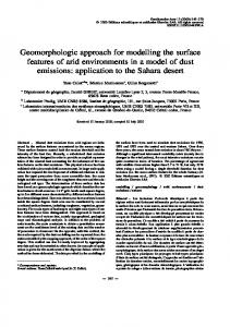
A domain of an arbitrary shape is illustrated in Fig. 1a. The domain is divided into three subdomains. Any scheme of subdivision, with various numbers, shapes and sizes of subdomains, can be used, as long as a scaling centre for each subdomain can be found from which the subdomain boundary is fully visible. Fig. 1b shows the details of Subdomain 1. The subdomain is represented by scaling a defining curve S relative to a scaling centre. The defining curve is usually taken to be the domain boundary, or part of the boundary. A normalised radial coordinate ξ is defined, varying from zero at the scaling centre and unit value on S. A circumferential coordinate s is defined around the defining curve S. A curve similar to S defined by ξ=0.5 is shown in Fig. 1b. The coordinates ξ and s form the local coordinate system, which is used in all the subdomains. One can see that the SBFEM represents a domain with subdomains whereas the FEM represents a domain with finite elements. Both the subdomains and the finite elements are represented by nodes on their edges. Nevertheless, three differences between the FEM and the SBFEM are evident: (i) the local coordinate system for a finite element is generally orthogonal in a particular coordinate space (e.g., the natural coordinate system in isoparametric elements), while the SBFEM coordinate system can be mapped to a polar coordinate system for each subdomain; (ii) the number of edges and the number of nodes can vary to a great extent from one subdomain to another. For example, the three subdomains in Fig. 1a have 7, 4 and 6 edges, and 14, 10 and 12 nodes respectively. Even the number of nodes in a same subdomain can vary from one edge to another. In contrast, it is unusual to use different types of finite elements in the same mesh in the FEM to discretise a domain unless absolutely necessary, and any one particular type of element has same number of nodes on each edge. This flexibility of SBFEM has recently been exploited to develop a simple remeshing procedure for mixed-mode crack propagation modelling by Yang [27]. This property is probably the reason that Song [22] has described subdomains as “super-elements”; and (iii) the edges connected to a scaling centre (e.g., Subdomain 1 and

5

Subdomain 3 in Fig. 1) do not need to be discretised even when they are subjected to displacement constraints or external loading [28]. The governing equilibrium equations of the SBFEM have been derived within the context of virtual work principle for elastostatics by Deeks and Wolf [29]. An extension to elastodynamics has also been made by Yang et al [26]. They are not repeated here. In a frequency-domain analysis, the first step is to compute the CFRFs. The governing equilibrium equations of the SBFEM under a harmonic excitation with constant frequency f (Hz), e.g. p=p0 ei2πft are [26] p 0 = E 0u(ξ ) ,ξ + E1 u(ξ ) ξ =1

(1)

E0ξ 2u(ξ ),ξξ + (E0 + E1 − E1 )ξu(ξ ),ξ − E 2u(ξ ) + (2πf ) 2 ξ 2M 0u(ξ ) = 0

(2)

T

T

where p0 are the magnitudes of the equivalent nodal loads. E0, E1, E2 and M0 are coefficient matrices that are dependent on the geometry of the subdomain boundaries and the material properties. u(ξ) represent the magnitudes of the nodal displacements and are analytical functions of the radial coordinate ξ. Eq. 1 and Eq. 2 first apply to subdomains. The contributions of subdomains to the coefficient matrices and equivalent nodal loads are then assembled in the same way as the contributions of finite elements in FEM. The assembled equation system for the whole domain has the same form as Eq. 1 and Eq. 2.

3. THE FROBENIUS SOLUTION PROCEDURE Eq. 2 is a second-order nonhomogeneous Euler-Cauchy differential equation system with respect to the radial coordinate ξ. The non-homogeneity complicates its solution considerably. An easy-to-follow analytical solution to Eq. 2 was recently developed by Yang et al [26] using the Frobenius procedure. Interested readers are referred to [26] for detailed derivation. The solution with (k+1) series is k +1

n

n

n

u = ∑ ciξ ( λi )φi + ∑ ξ ( λi )ci ( 2 g i ) +  ∑ ξ ( 1

i =1

2

i =1

i =1

k +1

λi )

ci ( k +1 g i )

(3)

where k +1

g i = k +1 G i φ i

(4a)

k +1

G i = k +1 B i k B i 2 B i

(4b)

k +1

B i = −(2πf ) 2 ( k +1λi ) 2 E0 +( k +1λi )(E1 − E1 ) − E 2 M 0

[

T

]

−1

(4c)

6

k +1

1

d i = k +1 B i ( k d i )

(4d)

d i = ci φ i

(4e)

λi = k λi + 2

k +1

(4f)

where the subscript i ranges from 1 to n for all the variables and n is the DOFs of the problem. Eq. 3 shows that the solution to elastodynamics consists of (k+1) summations of series. The first summation is the solution to the corresponding homogeneous equations of Eq. 2, i.e., the governing equations for elastostatics. The added k summations account for dynamic effects. More series terms are added, more accurately the solution represents the dynamic effects. 1λi = λi and φi are the positive eigenvalues and corresponding eigenvectors of the standard linear eigenproblem [29] formed from the elastostatic governing equations. ci are constants determined by boundary conditions. Eqs 4a-4f describe an iterative process in which the number of added summation terms k in Eq. 3 is determined by a convergence criterion [26]: max (|R|)< α

(5a) n

R = (2πf ) 2 M 0 ∑ ξ (

k +2

λ i ) k +1

(

i =1

(5b)

di )

where R can be regarded as the residual vector and α is the convergence tolerance. Setting ξ=1 in Eq. 3 leads to k +1

u ξ =1 = u b = Ψ 1c

or

−1

c = Ψ1 ub

(6)

where ub is the nodal displacements on the boundary, c={c1 c2 … cn}T and the matrix k +1

k +1

Ψ 1 = [(φ1 + ∑ j g1 )

(φ 2 + ∑ j g 2 )

j =2

k +1



j =2

(φ n + ∑ j g n )]

(7)

j =2

Substituting Eq. 3 into Eq. 1 leads to p 0 = E 0 Ψ 2 c + E1 Ψ 1c T

(8)

where the matrix k +1

Ψ 2 = [(1λ1φ1 + ∑ j g1 j λ1 ) j =2

k +1

(1λ2φ 2 + ∑ j g 2 j λ2 ) j =2

k +1



(1λn φ n + ∑ j g n j λn )]

(9)

j =2

Substituting Eq. 6 into Eq. 8 gives −1

p 0 = (E 0 Ψ 2 Ψ 1 + E1 )u b = K d u b T

(10)

7

Therefore, the dynamic stiffness matrix of the domain with respect to DOFs on the boundary is −1

K d = E 0 Ψ 2 Ψ 1 + E1

T

(11)

The nodal displacement vector ub can be calculated by Eq. 10 by applying boundary conditions on ub and loading conditions on p0. The integration constants c are then obtained using Eq. 6. Assuming the (k+1)th solution meets the criterion Eq. 5a, the displacement field is recovered as n n 1 2 k +1 n  u(ξ , s ) = N( s ) ∑ ciξ ( λi ) φ i + ∑ ξ ( λi ) ci ( 2 g i ) +  ∑ ξ ( λi ) ci ( k +1 g i ) i =1 i =1  i =1 

(12)

where N(s) is the matrix of shape functions at the circumferential direction, which are constructed as in FEM, typically using polynomial functions. The stress field is then obtained as n n k +1 2 1  n σ (ξ , s ) = DB1 ( s ) ∑ ci (1λi )ξ ( λi −1) φ i + ∑ ci ( 2λi )ξ ( λi −1) ( 2 g i ) +  ∑ ci ( k +1λi )ξ ( λi −1) ( k +1 g i ) i =1 i =1  i =1  (13) n n  n (1λi −1) ( 2λi −1) 2 ( k +1λi −1) k +1 2 + DB ( s ) ∑ ciξ ( g i ) +  ∑ ciξ ( g i ) φ i + ∑ ciξ i =1 i =1  i =1 

where D is the elasticity matrix and B1(s) and B2(s) are relevant matrices [17]. One can see that the dynamic displacement and stress fields from the SBFEM (Eq. 12 and Eq. 13) are analytical with respect to the radial coordinate ξ. Therefore, these state variables at any position of the domain can be directly calculated once the nodal displacements on the boundary are obtained by solving Eq. 10. In contrast, to obtain state variables at a desired position in the FEM, a node must be added at this position. This may lead to very small elements if the desired position is close to the boundary.

4. CALCULATION OF TRANSIENT RESPONSE BY FAST FOURIER TRANSFORM The frequency-domain analysis is a well established method. A brief introduction to the FFT and IFFT is given in this section as a reference point for the following discussion. Consider a periodic excitation force p(t) defined by N number of discrete values pn=p(tn)=p(nΔt) where Δt=T0/N is the sampling interval, T0 is the period and n ranges from 0 to N-1. The array pn describing the discretised force function can be expressed as a superposition of N harmonic functions

8

N −1

N −1

j =0

j =0

pn = ∑ Pj ei ( j 2πf 0 t n ) = ∑ Pj ei ( 2πnj / N ) , n = 0,, N − 1

(14)

where f0=1/T0 is the frequency (Hz) of first harmonic in the periodic extension of p(t), fj=j·f0 is the frequency of the jth harmonic, and Pj is a complex-valued coefficient that defines the amplitude and phase of the jth harmonic. Pj can be expressed as Pj =

1 N

N −1

∑ pne−i ( j 2πf 0t n ) = n=0

1 N

N −1

∑p e n=0

− i ( 2πnj / N )

n

,

j = 0,, N − 1

(15)

Eq. 14 and Eq. 15 define a discrete Fourier transform (DFT) pair: the array Pj is the DFT of the excitation sequence pn, and the array pn is the inverse of DFT (IDFT) of the sequence Pj. The frequency of the highest harmonic included in Eq. 14 and Eq. 15 is known as the Nyquist frequency and is given by N·f0/2 = 1/(2Δt). For each f=fj (0≤j≤N/2), a complex frequency-response function Hj is computed. Because Eq. 14 is a one-sided Fourier expansion, the values of Hj on either side of j=N/2 must be complex conjugates of each other, i.e., H j = H N* − j ,

j=

N + 1,, N − 1 2

(16)

where H* denotes the complex conjugate of H. The response to each harmonic component of the excitation can be calculated as U j = H j Pj ,

j = 0,, N − 1

(17)

Finally, the response un=u(tn) at discrete time instants tn=nΔt is computed by the IDFT of Uj N −1

N −1

j =0

j =0

un = ∑U j ei ( j 2πf 0 t n ) = ∑U j ei ( 2πnj / N ) , n = 0,, N − 1

(18)

The above is the classical DFT solution in the frequency domain to the transient elastodynamics. It became a practical solution method only with the publication of the CooleyTukey algorithm for the FFT in 1965 [30], which is a highly efficient and accurate method of computing the DFT-IDFT pair.

5. NUMERICAL EXAMPLES, RESULTS AND DISCUSSION Six transient dynamic examples subjected to various forms of transient loadings are modelled in this study using the developed frequency-domain method based on the SBFEM. For each example, the CFRFs of displacements or stresses at desired positions in the domain are first computed for a wide range of sampling frequencies fj(j=1, …, M) using the Frobenius solution

9

procedure presented in Section 3. The minimum frequency is f1=0Hz (static case) and the maximum is fM=fmax, with an frequency interval Δf=fmax/(M-1). A FFT of the transient load (Eq. 15) is then carried out to obtain the coefficients Pj(j=0, …, N-1). The frequency responses Hj(j=0, …, N/2) are then interpolated from the M number of sampling responses. The interpolation is usually necessary because a much greater N (an integer power of 2) may be needed to accurately represent the transient load whereas the CFRFs can be reasonably represented by a smaller M number of frequencies. This may save considerable computing cost. The full frequency-response functions are then completed by Eq. 16. Finally, an inverse FFT (Eq. 18) of Uj(j=0, …, N) calculated by Eq. 17 is carried out to obtain un(n=0, …, N), i.e., the time history of displacement or stress at desired positions. The functions fft() and ifft() in MATLAB [31] are used to conduct FFT and IFFT respectively. For each example, the same CFRFs are used to calculate time histories for all the forms of transient loadings that this example is subjected to. The damping effect is taken into account by modifying the elastic moduli to incorporate an internal damping coefficient β as in [23], forming the complex Young’s modulus Ec=E(1+i2β) and the complex shear modulus Gc=G(1+i2β), where E and G are the elastic Young’s modulus and the elastic shear modulus respectively. A suitable damping coefficient β is very important in the frequency-domain approach. A too small β may lead to oscillation in the time responses whereas a high β may cause over-damping and thus underestimate the time responses. Because the material properties are different in the numerical examples, parametric studies are carried out to determine a proper β for each example. Because the FFT and IFFT are highly efficient, most of the computational time is spent on calculating the CFRFs using the Frobenius solution procedure. Therefore, the maximum frequency fmax and the frequency interval Δf, determining the CFRFs, must be rationally selected in order to achieve both sufficient accuracy and reasonable efficiency. For such purpose, a linear perturbation analysis is carried out using the finite element analysis package ABAQUS [32] to extract the first 20 natural frequencies for each example. It was found that for all examples modelled in this study, the CFRFs including frequencies up to the 10th natural frequency and those including up to the 20th led to little difference to the time responses. Therefore, fmax of a slightly higher value than the 10th natural frequency is used for all the examples modelled. A suitable frequency interval Δf is also decided by trying a few values for each example. In FFT and IFFT, N=211=2048 is used for all the analyses in this study. This ensures an accurate

10

representation of the transient loading in FFT (Eq. 15) and also accurate calculation of responses in IFFT (Eq. 18). A transient dynamic finite element analysis using ABAQUS is also carried out for all the examples for comparison. The explicit time-integration scheme is used for the second example and the implicit scheme is used for all the others [32]. No physical damping (i.e., pure elastic material behaviour) is considered in all the finite element analyses. The international standard unit system, namely mass in kilograms, length in metres and time in seconds, is used for all the examples and thus no units are indicated with all the physical entities. Two-node linear line elements and α=0.001 in Eq. 5a are used for all the analyses using the SBFEM. A plane stress condition is assumed for all the examples. Quantitative comparisons of the proposed method with the FEM, the BEM and the timedomain SBFEM [22] are not conducted with respect to the computational costs, as the results would be influenced greatly by the algorithms used in the many different steps in the respective methods.

5.1 Example 1: 1D rectangular rod The first example solved here is the classical wave propagation problem, which was modelled by many using the BEM [7-9] and the BEM/FEM coupled method [11, 12]. A rectangular rod is subjected to a uniform traction on the right end with the left end fixed. The geometry, boundary and loading conditions are shown in Fig. 2a. The zero Poisson’s ratio imposes the one-dimensional condition. The width of the rod does not affect the results. Two loading forms are modelled for this example: a Heaviside step function representing a suddenly applied load and a triangular function representing a blast load, as shown in Fig. 2a. The time responses at the points A, B and C in Fig. 2a are examined. Only one subdomain is used to model this example. Fig. 2b shows a typical mesh with only 15 nodes. The scaling centre is placed at the left-bottom corner so that the two edges connected to it are not discretised. Very small material damping coefficient β, ranging from 1e-8 to 1e-6, was found to yield stable results. This is because the Young’s modulus E=1 is so small in this example that a higher β causes over-damping and thus underestimates the results considerably. All the results presented below for this example are from β=1e-6. Fig. 3 and Fig. 4 show the time histories of the horizontal (axial) displacements at the free end of the rod (the point A) and the middle of the rod (the point B) respectively under the

11

Heaviside step load. The results from both the frequency-domain SBFEM and the time-domain FEM are in very good agreement with the analytical solutions [33]. The axial stress histories at the middle and the fixed end of the rod are shown in Fig. 5 and Fig. 6 respectively. Good agreement between the numerical results and the analytical solution can also be observed, except that the FEM results oscillate fiercely around the analytical solutions at moments when the stress jumps. This is caused by the sudden application of the step load and cannot be completely corrected by numerical measures. It also happens in other studies [7-9, 11-12]. The oscillations also appear in the results from the frequency-domain approach, but with lower magnitudes and much less degree. It looks that this approach tends to average responses at the discontinuous time points so as to yield much smoother curves (see Figs. 3-6). This may be caused by the material damping used in the approach. Fig. 7 compares the horizontal displacement histories at the points A and B under the triangular blast load. The results from the two numerical methods are virtually identical. Excellent agreement can also be seen in the axial stress histories at the middle and the fixed end of the rod, which are presented in Fig. 8 and Fig. 9 respectively. No oscillation happens because the triangular blast load function is continuous. Figs 7-9 can be compared with the results calculated from the BEM/FEM coupling method in [12].

5.2 Example 2: 1D segmented rectangular rod with a bi-material interface The second example is a 1D segmented rod made up of two materials: one half is the steel and the other the aluminium. This example was recently modelled by Batra et al [15] using a meshless Petrov-Galerkin formulation. The same dimensions, boundary and loading conditions as in [15] are used in this study (Fig. 10a). The uniform traction applied on the left free end has the form of a sinusoidal pulse. The time responses at the points A and B in Fig. 10a are investigated. Fig. 10b shows a mesh consisting of only 33 nodes. Only one subdomain is used to model this bi-material example. The scaling centre is placed at the middle-bottom so that the bottom edge is not discretised. The bi-material interface connected to the scaling centre does not need discretisation either, because the displacement gradient discontinuity on the interface is automatically satisfied by the analytical displacement solution (Eq. 12), so is the stress continuity on the interface. One may notice that for the meshless method, special treatments such as the Lagrange multipliers or jump functions as used in [15], are necessary to impose the displacement

12

gradient discontinuity and thus the stress continuity at the interface. No special treatment is needed in the SBFEM. The existence of the material interface complicates the wave propagation behaviour considerably. Fig. 11 and Fig. 12 show the axial displacement histories calculated from the explicit FEM and the frequency-domain method using β=1e-3 at the points A and B respectively. Overall agreement between the two numerical methods is good, although local discrepancies occur. The slight difference between Fig. 11 here and Fig. 13 in [15] may come from the approximation of the sinusoidal blast load by ten straight lines as input for both numerical analyses in this study. The axial stress histories at the point B and the point C are shown in Fig. 13 and Fig. 14 respectively. Again very good overall agreement is observable.

5.3 Example 3: 2D cantilever beam The third example is a 2D cantilever beam as shown in Fig. 15. This forced vibration problem has the same dimensions, boundary conditions and material properties as the first example except that the Poisson’s ration of the material is 0.3. The beam is subjected to uniform traction at its upper surface. The time responses at the points A and B in Fig. 15 are examined. The same problem subjected to Heaviside step load was modelled in [11] using the BEM/FEM coupling method. The same mesh as in Fig. 2b is used to model this example. The material damping coefficient β=1e-6 is used. The transient responses under the Heaviside step load and the triangular blast load (Fig. 15) are calculated using the FEM and the SBFEM. Fig. 16 and Fig. 17 show the vertical displacement histories at the point B and the horizontal stress histories at the point A respectively from the Heaviside step load. The results from the blast load are shown in Fig. 18 and Fig. 19. Again there is excellent agreement between the results from the FEM and those from the SBFEM. As the first example, considerable oscillations happen to the stress history calculated by the FEM under the Heaviside step load whereas much smoother responses are obtained by the developed frequency-domain method (Fig. 17).

5.4 Example 4: 2D simply-supported beam subjected to uniform bending force The forced vibration of a 2D simply-supported beam is modelled as the 4th example. The dimensions, boundary and loading conditions, and material properties are illustrated in Fig. 20a. The beam is subjected to a uniformly-distributed bending traction at its upper face. The time

13

responses at the points A and B in Fig. 20a are examined. Both the Heaviside step load and the blast load (only the latter is shown in Fig. 20a) are modelled. The same beam subjected to the Heaviside step load was modelled by Zienkiewicz et al [34] using the time-domain FEM. The beam is modelled with two subdomains consisting of totally 33 nodes using the SBFEM as shown in Fig. 20b. The two scaling centres are positioned at the beam lower face so that this whole face is not discretised. A material damping coefficient β=1e-5 is used. Fig. 21 and Fig. 22 show the vertical displacement histories at the point B and the horizontal stress histories at the point A respectively under the Heaviside step load. Also shown in these figures are the analytical solutions [33] taking the effects of rotary inertia and shear deformation into account. It is evident that the results from the time-domain FEM and the frequency-domain SBFEM almost coincide with each other, and the results from both methods agree very well with the analytical solutions, especially for the displacement histories. Because the stresses are derivatives of displacements and thus less accurate, the discrepancies between the analytical stress solution and the numerical results are understandable. Comparing the results here with those reported in [34] also confirms the effectiveness and accuracy of the developed frequencydomain SBFEM. The same conclusion can also be drawn from the results under the blast load, which are shown in Fig. 23 and Fig. 24.

5.5 Example 5: 2D simply-supported beam subjected to concentrated force This example is same as the 4th example except that the beam is subjected to a concentrated force at the half span on the upper face as shown in Fig. 25. The same mesh as in Fig. 20b is used with β=1e-5. Again, good agreement between the results from the frequency-domain SBFEM and the time-domain FEM, and between those from numerical methods and the analytical solution [33], is obtained, as demonstrated by Figs 26-29. As in all the above examples, the displacement histories simulated by the two numerical methods are smooth under both the Heaviside step load and the blast load (Fig. 26 and Fig. 28). The stress results from the time-domain FEM, however, show significant oscillations under both the Heaviside step load (Fig. 27) and the blast load (Fig. 29), which do not occur for the beam subjected to the uniformly-distributed load in the previous example. This could be attributed to the concentrated load in this example, which causes stress concentration around the loading point. This stress concentration, in turn, causes local numerical instabilities in the time-integration based FEM. The stress concentration, however, appears not to

14

adversely affect the ability of the new frequency-domain approach to compute smooth curves of time responses.

5.6 Example 6: 2D frame-like structure subjected to wind load The final example is a frame-like structure, which was modelled by Sladek et al [13] using the meshless method. The dimensions, boundary and loading conditions, and material properties are illustrated in Fig. 30a. The frame is fixed at the two bottom edges and subjected to a uniformly-distributed traction in the form of a ramped wind load at the left face. The displacement histories at the points A and B are investigated. The frame is modelled with two subdomains consisting of totally 41 nodes using the SBFEM as shown in Fig. 30b. The two scaling centres are positioned at the two corners with stress concentration. Because the solutions in the SBFEM are analytical, the stress concentration is automatically represented without any refinement in the mesh. A material damping coefficient β=1e-4 is used. Good agreement can be seen between the displacement histories predicted by the FEM and the SBFEM at the point A and the point B, as shown in Fig. 31 and Fig. 32 respectively. The results in Fig. 31 are comparable with Fig. 7 in [13].

6. CONCLUSIONS A frequency-domain approach using the SBFEM has been developed in this study for modelling general transient dynamic problems. The newly-developed analytical Frobenius solution to the governing equations of SBFEM is first applied for a wide range of frequencies, leading to complex frequency-response functions. These functions are subsequently used by the FFT and the IFFT to calculate time histories of structural responses. This new approach does not need a mass matrix which is a low-frequency expansion of the dynamic stiffness matrix, as needed by the time-domain SBFEM, and thus allows a structure to be modelled by fewer subdomains efficiently without loss of accuracy. Extensive transient dynamic analyses of six examples have been successfully carried out using the new method. The fact that these examples have quite different dynamic behaviour, geometries, materials properties, boundary conditions and are subjected to various transient load forms, demonstrates the high generality and wide applicability of this method. The fact that all these examples are successfully modelled with very small number of DOFs should be attributed

15

to the analytical nature of the Frobenius solutions. Although much remains to be done in comparing the numerical efficiency between this method and the others, its numerical stability appears to be consistently ensured if a suitable material damping coefficient is selected. An expansion of the Frobenius solution procedure to consider unbounded domains will allow this frequency-domain SBFEM to model dynamic soil-structure interaction. This work is currently underway.

ACKNOWLEDGEMENT This research is supported by the Australian Research Council (Discovery Project No. DP0452681) and the National Natural Science Foundation of China (No. 50579081).

REFERENCES [1] Zienkiewicz OC and Taylor RL. The finite element method. 5th edition. ButterworthHeinemann. 2000. [2] Dokainish MA, Subbaraj K. A survey of direct time-integration methods in computational structural dynamics—I. Explicit methods. Computers & Structures 1989; 32(6):1371-1386. [3] Subbaraj K, Dokainish MA. A survey of direct time-integration methods in computational structural dynamics—II. Implicit methods. Computers & Structures 1989; 32(6):1387-1401. [4] Murti V, Valliappan S. The use of quarter point element in dynamic crack analysis. Engineering Fracture Mechanics 1986; 23(3):585-614. [5] Wiberg NE, Zeng LF, Li XD. Error estimation and mesh adaptivity for elastodynamics. Computer Methods in Applied Mechanics and Engineering 1992; 101:369-395. [6] Zeng LF, Wiberg NE. Spatial mesh adaptation in semidiscrete finite element analysis of linear elastodynamics problems. Computational Mechanics 1992; 9:315-332. [7] Carrer JAM, Mansur WJ. Alternative time-marching schemes for elastodynamic analysis with the domain boundary element method formulation. Computational Mechanics 2004; 34(5):387-399. [8] Carrer JAM, Mansur WJ. Time discontinuous linear traction approximation in time-domain BEM: 2-D elastodynamics. International Journal for Numerical Methods in Engineering 2000; 49(6):833-848.

16

[9] Wang CC, Wang HC, Liou GS. Quadratic time domain BEM formulation for 2D elastodynamic transient analysis. International Journal of Solids and Structures 1997; 34(1):129-151. [10]

Tanaka M, Chen W. Dual reciprocity BEM applied to transient elastodynamic problems

with differential quadrature method in time. Computer Methods in Applied Mechanics and Engineering 2001; 190(18-19). [11]

Yu GY, Mansur WJ, Carrer JAM. A more stable scheme for BEM/FEM coupling applied

to two-dimensional elastodynamics. Computers & Structures 2001; 79(8):811-823. [12]

Chien CC, Wu TY. A particular integral BEM/time-discontinuous FEM methodology for

solving 2-D elastodynamic problems. International Journal of Solids and Structures 2001; 38(2):289-306. [13]

Sladek J, Sladek V, Van Keer R. Meshless local boundary integral equation method for

2D elastodynamic problems. International Journal for Numerical Methods in Engineering 2003; 57(2):235-249. [14]

Gu YT, Liu GR. A meshless local Petrov–Galerkin (MLPG) method for free and forced

vibration analyses for solids. Computational Mechanics 2001; 27188–198. [15]

Batra RC, Porfiri M, Spinello D. Free and Forced Vibrations of a Segmented Bar by a

Meshless Local Petrov–Galerkin (MLPG) Formulation. Computational Mechanics 2006; published online. DOI: 10.1007/s00466-006-0049-6. [16]

Wolf JP, Song CM. Finite-element modelling of unbounded media. Chichester: John

Wiley and Sons, 1996. [17]

Wolf JP. The scaled boundary finite element method. Chichester: John Wiley and Sons,

2003. [18]

Zhang X, Wegner JL, Haddow JB. Three-dimensional dynamic soil-structure interaction

analysis in the time domain. Earthquake Engineering & Structural Dynamics 1999; 28(12):1501-1524. [19]

Yan JY, Zhang CH, Jin F. A coupling procedure of FE and SBFE for soil-structure

interaction in the time domain. International Journal for Numerical Methods in Engineering 2004; 59(11):1453-1471. [20]

Ekevid T, Wiberg NE. Wave propagation related to high-speed train - A scaled boundary

FE-approach for unbounded domains. Computer Methods in Applied Mechanics and Engineering 2002; 191(36):3947-3964.

17

[21]

Genes MC, Kocak S. Dynamic soil-structure interaction analysis of layered unbounded

media via a coupled finite element/boundary element/scaled boundary finite element model. International Journal for Numerical Methods in Engineering 2005; 62(6):798-823. [22]

Song CM. A super-element for crack analysis in the time domain. International Journal

of Numerical Methods in Engineering 2004; 61(8):1332-1357. [23]

Spyrakos CC, Beskos DE. Dynamic response of frameworks by fast Fourier transform.

Computers & Structures 1982; 15(5): 495-505. [24]

Polyzos D, Tsepoura KG, Beskos DE. Transient dynamic analysis of 3-D gradient elastic

solids by BEM. Computers & Structures 2005; 83(10-11):783-792. [25]

Song CM, Wolf JP. The scaled boundary finite-element method: analytical solution in

frequency domain. Computer Methods in Applied Mechanics and Engineering 1998; 164(12): 249-264. [26]

Yang ZJ, Deeks AJ and Hao H. A Frobenius Solution to the Scaled Boundary Finite

Element Equations in Frequency Domain. International Journal of Numerical Methods in Engineering. Under review. [27]

Yang ZJ. Fully automatic modelling of mixed-mode crack propagation using scaled

boundary finite element method. Engineering Fracture Mechanics, in press. [28]

Deeks AJ. Prescribed side-face displacements in the scaled boundary finite-element

method. Computers & Structures 2004; 82(15-16):1153-1165. [29]

Deeks AJ, Wolf JP. A virtual work derivation of the scaled boundary finite-element

method for elastostatics. Computational Mechanics 2002; 28(6):489–504. [30]

Cooley JW, Tukey JW. An algorithm for the machine calculation of complex Fourier

series. Mathematics of Computation 1965; 19:297-301. [31]

MATLAB V7.1. The MathWorks, Inc, 2005.

[32]

Hibbitt, Karlsson and Sorensen Inc. ABAQUS/Standard User Manual V6.5, 2004.

[33]

Timoshenko S, Young DH, Weaver W. Vibration Problems in Engineering. 4th edition,

John Wiley & Sons, 1974. [34]

Zienkiewicz OC, Li XK, Nakazawa S. Dynamic transient analysis by a mixed, iterative

method. International Journal for Numerical Methods in Engineering 1986; 23(7):1343-1353.

18

s

1

P

s=s1

Side faces Radial lines

1 s=s0

3 2

y

Scaling centre (ξ=0) y 2-noded elements x

x

Scaling centres

Nodes

ξ

Defining curve S (ξ 1) Similar curve to S (ξ=0.5)

Internal boundaries a) Subdomaining of a domain

b) Subdomain 1

Fig. 1. The concept of the scaled boundary finite-element method

0.5

E=1, ρ=1, ν=0, t=1, P0=1, plane stress C

B

P P0 t

P0

P

A

P

1 2 t Blast loading

Heaviside loading

1.0

a) Dimensions, material properties and loading

b) A mesh with 15 nodes

conditions Fig. 2 Example 1: a 1D rectangular rod

19

Horizontal displacement at point A

2

Analytical FEM Present

1.8 1.6 1.4 1.2 1 0.8 0.6 0.4 0.2 0 0

2

4

6

8

10

12

Time

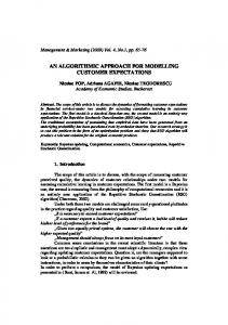
Fig. 3 Horizontal displacement at the point A under the Heaviside step load for the 1st example

Horizontal displacement at point B

1.1 1 0.9 0.8 0.7 0.6 0.5 0.4 0.3 0.2 0.1 0

Analytical

-0.1 0

2

FEM 4

6

Present 8

10

12

Time

Fig. 4 Horizontal displacement at the point B under the Heaviside step load for the 1st example

20

Horizontal stress at point B

2.5

Analytical FEM Present

2 1.5 1 0.5 0 -0.5 0

2

4

6

8

10

12

Time

Fig. 5 Horizontal stress at the point B under the Heaviside step load for the 1st example 2.7

Horizontal stress at point C

2.3 1.9 1.5 1.1 0.7 0.3 -0.1 -0.5

Analytical

-0.9 0

2

4

FEM 6

Present 8

10

1

Time

Fig. 6 Horizontal stress at the point C under the Heaviside step load for the 1st example

21

1

Horizontal displacements

0.75 0.5 0.25 0 -0.25

FEM (A) Present (A) FEM (B) Present (B)

-0.5 -0.75 -1 0

2

4

6

8

10

12

Time

Fig. 7 Horizontal displacements at the point A and B under the blast load for the 1st example

1.2

Horizontal stress at point B

0.9 0.6 0.3 0 -0.3

FEM

-0.6

Present

-0.9 -1.2 0

2

4

6

8

10

12

Time

Fig. 8 Horizontal stress at the point B under the blast load for the 1st example

22

2

Horizontal stress at point C

1.5 1 0.5 0 -0.5

FEM

-1

Present -1.5 -2 0

2

4

6

8

10

12

Time

Fig. 9 Horizontal stress at the point C under the blast load for the 1st example

Material 2

E1=2e11, ρ1=7860, A E1=7e10, ρ2=2710, ν1= ν2=0, t=1, P0=1e8

P

A

P(t)=P0sin(πt/t0) P0

0.025

Material 1

B t0=3.95 t(μs) Blast loading

0.05 B

a) Dimensions, material properties and loading

b) A mesh with 33 nodes

conditions Fig. 10 Example 2: a 1D segmented rectangular rod with a bi-material interface

23

Horizontal displacement at point A

1.40E-05 1.20E-05 1.00E-05 8.00E-06 6.00E-06 4.00E-06 2.00E-06 0.00E+00 -2.00E-06 -4.00E-06 -6.00E-06 -8.00E-06 -1.00E-05 -1.20E-05 -1.40E-05 0.00E+00

FEM Present

2.00E-05

4.00E-05

6.00E-05

8.00E-05

Time

Fig. 11 Horizontal displacement at the point A under the sinusoidal blast load for the 2nd example

Horizontal displacement at point A

1.20E-05 1.00E-05

FEM

8.00E-06

Present

6.00E-06 4.00E-06 2.00E-06 0.00E+00 -2.00E-06 -4.00E-06 -6.00E-06 -8.00E-06 -1.00E-05 -1.20E-05 0.00E+00

2.00E-05

4.00E-05

6.00E-05

8.00E-05

Time

Fig. 12 Horizontal displacement at the point B under the sinusoidal blast load for the 2nd example

24

1.20E+08

FEM Present

Horizontal stress at point B

1.00E+08 8.00E+07 6.00E+07 4.00E+07 2.00E+07 0.00E+00 -2.00E+07 -4.00E+07 -6.00E+07 -8.00E+07 -1.00E+08 -1.20E+08 0.00E+00

2.00E-05

4.00E-05

6.00E-05

8.00E-05

Time

Fig. 13 Horizontal stress at the point B under the sinusoidal blast load for the 2nd example 1.20E+08

FEM Present

Horizontal stress at point C

1.00E+08 8.00E+07 6.00E+07 4.00E+07 2.00E+07 0.00E+00 -2.00E+07 -4.00E+07 -6.00E+07 -8.00E+07 -1.00E+08 -1.20E+08 0.00E+00

2.00E-05

4.00E-05

6.00E-05

8.00E-05

Time

Fig. 14 Horizontal stress at the point C under the sinusoidal blast load for the 2nd example

25

P E=1, ρ=1, ν=0.3, t=1, P0=1, plane stress

0.5

P

P0

P0 t Heaviside loading

A

P

3 6 t Blast loading

A 1.0

B

Fig. 15 Exampe 3: a cantilever beam

Vertical displacement at point B

32

Present FEM

28 24 20 16 12 8 4 0 -4 0

5

10

15

20

25

30

35

40

Time

Fig. 16 Vertical displacement at the point B under the Heaviside step load for the 3rd example

26

8

Horizontal stress at point A

Present FEM 6

4

2

0

-2 0

5

10

15

20

25

30

35

40

Time

Fig. 17 Horizontal stress at the point A under the Heaviside step load for the 3rd example

Vertical displacement at point B

20 16

Present

12

FEM

8 4 0 -4 -8 -12 -16 -20 0

5

10

15

20

25

30

35

40

Time

Fig. 18 Vertical displacement at the point B under the blast load for the 3rd example

27

Horizontal stress at point A

5 4

Present

3

FEM

2 1 0 -1 -2 -3 -4 -5 0

5

10

15

20

25

30

35

40

Time

Fig. 19 Horizontal stress at the point A under the blast load for the 3rd example

2

P E=9800, ρ=1, ν=0.15, t=1, P0=1, plane stress

P

P0

B A

0.1 0.2 t Blast loading

10 a) Dimensions, material properties and loading conditions

b) a mesh with 33 nodes Fig. 20 Example 4: a simply-supported beam subjected to uniformly distributed force

28

0.005 Vertical displacement at point B

0 -0.005 -0.01 -0.015 -0.02 -0.025 -0.03 -0.035 -0.04 -0.045

Analytical

-0.05 0

1

Present

2

FEM

3

4

5

Time

Fig. 21 Vertical displacement at the point B under the Heaviside step load for the 4th example 50

Analytical

Horizontal stress at point A

45

Present

FEM

40 35 30 25 20 15 10 5 0 -5 -10 0

1

2

3

4

5

Time

Fig. 22 Horizontal stress at the point A under the Heaviside step load for the 4th example

29

Vertical displacement at point B

0.015

Present

0.012

FEM

0.009 0.006 0.003 0 -0.003 -0.006 -0.009 -0.012 -0.015 0

1

2

3

4

5

Time

Fig. 23 Vertical displacement at the point B under the blast load for the 4th example 14

Present

FEM

Horizontal stress at point A

10.5 7 3.5 0 -3.5 -7 -10.5 -14 0

1

2

3

4

5

Time

Fig. 24 Horizontal stress at the point A under the blast load for the 4th example

30

2

P E=9800, ρ=1, ν=0.15, t=1, P0=1, plane stress

P0

B

P

0.1 0.2 t Blast loading

A

Fig. 25 Example 5: a simply-supported beam subjected to concentrated force

Vertical displacement at point B

0

-0.002

-0.004

-0.006

Analytical

Present

FEM

-0.008 0

1

3

2

4

5

Time

Fig. 26 Vertical displacement at the point B under the Heaviside step load for the 5th example

31

Horizontal stress at point A

7.5

6

4.5

3

1.5

0

Present

Analytical

FEM

-1.5 0

1

2

3

4

5

Time

Fig. 27 Horizontal stress at the point A under the Heaviside step load for the 5th example

0.0025 Vertical displacement at point B

Present

FEM

0.002 0.0015 0.001 0.0005 0 -0.0005 -0.001 -0.0015 -0.002 0

1

2

3

4

5

Time

Fig. 28 Vertical displacement at the point B under the blast load for the 5th example

32

2.5

Present

FEM

Horizontal stress at point A

2 1.5 1 0.5 0 -0.5 -1 -1.5 -2 0

1

2

3

4

5

Time

Fig. 29 Horizontal stress at the point A under the blast load for the 5th example

A

E=10000, ρ=1, ν=0.2, t=1, P0=10, plane stress

P

2

P0

0.1 t Wind loading

P

2

B

2

2

2

a)Dimensions, material properties and loading

b) a mesh with 41 nodes

conditions

Fig. 30 Example 6: a frame-like structure

33

Horizontal displacement at point A

0.02

FEM Present

0.018 0.016 0.014 0.012 0.01 0.008 0.006 0.004 0.002 0 0

0.1

0.2

0.3

0.4

0.5

0.6

0.7

0.8

0.9

1

Time

Fig. 31 Horizontal displacement at the point A under the ramped wind load for the 6th example

Horizontal displacement at point B

0.007

FEM Present

0.006 0.005 0.004 0.003 0.002 0.001 0 0

0.1

0.2

0.3

0.4

0.5

0.6

0.7

0.8

0.9

-0.001 Time

Fig. 30 Horizontal displacement at the point B under the ramped wind load for the 6th example

34