School of Engineering, Vanderbilt University, Nashville, TN 37235. {thongcs,goldfarb,sarkar,kawamura}@vuse.vanderbilt.edu. Abstract. This paper presents the ...
��������� � � � ����� � ���� ������ ��� ��� �� ����� ��������������
A Frequency Modeling Method of Rubbertuators for Control Application in an IMA Framework S. Thongchai∗ M. Goldfarb∗∗ N. Sarkar∗∗ and K. Kawamura∗ ∗ Department of Electrical Engineering ∗∗ Department of Mechanical Engineering School of Engineering, Vanderbilt University, Nashville, TN 37235 {thongcs,goldfarb,sarkar,kawamura}@vuse.vanderbilt.edu Abstract This paper presents the results of rubbertuator modeling for purposes of control applications. A pair of rubbertuators is constructed as a revolute joint. The rubbertuator arm is highly nonlinear and exhibits hysteresis. The frequency modeling method was implemented using software agents within the Intelligent Machine Architecture (IMA) framework. Several linear models were built, simulated, and employed to design a controller for the rubbertuators. The results show that all models match the experimental data in each frequency range. A fuzzy model-based controller was designed and implemented as an example using the IMA framework.
1 Introduction Several robots have been developed in the Intelligent Robotics Laboratory (IRL) at Vanderbilt University. The Soft Arm robot named ISAC (Intelligent Soft Arm Control), is the main robot. ISAC consists of two rubbertuator-based humanoid arms and a pan-tiltverge binocular vision system. The rubbertuator, also called a McKibben artificial muscle, is a very compliant actuator, however it is also highly nonlinear [8]. Because of the natural compliance of rubbertuators, ISAC is well suited for operation near in close proximately of humans [4]. The trade-off is lower speed, lower accuracy, and more difficult control [1]. This paper is concerned with the frequency response modeling and control of the rubbertuator system. The response is limited by the physics of pneumatic actuators, which is quite slow compared to servo-motor actuators. Both frequency and gain are obtained from the experiments. The results from frequency-domain technique can be considered as linear models. The availability of the dynamic model is useful for controller design and computer simulation. The Soft Arm robot can be shown modeled using both linear and nonlinear models. Several linear models can be used as a nonlinear model, which can be applied to
multiple model approaches [3]. The experiment was setup in the Intelligent Machine Architecture (IMA) framework developed in the IRL [9]. The Soft Arm is tested with sine-wave input. A number of frequencies are varied in the interesting frequency band. Finally, three linear models are obtained. A model-based fuzzy controller is designed using a linear model. The example shows that the model can be used to design a good controller.
2 Overview 2.1 The Intelligent Machine Architecture The Intelligent Machine Architecture (IMA) is an agent-based software system for developing intelligent robot control, designed in the IRL at Vanderbilt University, that permits the concurrent execution of software agents on separate machines while facilitating extensive inter-agent communication. The IMA is a new approach for the design of the control software for intelligent machines that are principally limited by difficulty in integrating existing algorithms, models, and subsystems [9]. It can be used to implement virtually any robot control architecture and provides a two-level software framework for the development of intelligent machines. The robot-environment level describes the system structure in terms of a group of atomic software agents connected by a set of agent relationships. The agent-object level describes each of the atomic agents and agent relationships as a network of software modules called component objects. At the robotenvironment level, IMA defines several classes of atomic agents and describes their primary functions in terms of environmental models, behaviors or tasks. Sensor and actuator agents provide abstractions of sensors and actuators and incorporate basic processing and control algorithms. 2.2 Rubbertuator-Based Robot The rubbertuators are pneumatically actuated. They are also known as McKibben artificial muscles. The IRL’s Intelligent Soft Arm Control (ISAC) robot
uses the Soft-Arm manipulator as shown in Figure 1. This manipulator is modeled from the human arm and has four joints resulting in six degrees of freedom. Each robot joint consists of two rubbertuators that function as the muscles in the human arm. If pressure inside one of the rubbertuators increases, pressure in the other one decreases, and the manipulator link moves because of the expansion and contraction of the actuators.
output. The frequency response function of a linear system can be described as the first-order system G (jω) =
1 (1 + jωτ )
(1)
and the standard second-order system G (jω) = 1−
³
ω ωn
´2
1 + j2ζ
³
ω ωn
(2)
´
where ω³is the ´ natural frequency, ωn is the corner freω quency, ωn is the normalized frequency, and ζ is the damping ratio. The value of damping ratio (ζ) can be selected from the standard response of second-order system, which can be found in many control textbooks such as Ogata [7] and Rohrs et al. [11].
3 Soft Arm Modeling: Experimental Results
Figure 1: ISAC humanoid robot Due to the rubbertuators performing as a complex behavior, highly nonlinear, and hysteresis system, the modeling and control of this system is difficult. This paper presents the frequency modeling method with application of model-based control techniques. 2.3 Frequency Modeling Technique Although, in practice, most physical systems are nonlinear with distributed parameters, they can be approximated as linear systems. Linear models for such systems are often used because of their simplicity and usefulness in designing a controller. There are many models that can be obtained by using system identification techniques [6]. However, for practical purposes, some complex systems may not be applied. A simple method for obtaining detailed information about a linear system is called frequency analysis. The frequency modeling method is a practical technique that can be used to find the rubbertuator models. Frequency response identification is the determination of the system transfer function from experimental measurements [6]. The transfer function of the system models can be built from the frequency response information. The frequency response function can be sketched as magnitude and phase, which is called bode plot. The transfer functions are useful for linear systems, which can be presented as the ratio of input and
The Soft Arm is tested in the IMA framework. The input of the rubbertuator is the difference pressure, varying from -2000 to 2000 points. The input frequency varies from 0.01-1.5 Hz. The amplitude for each frequency is varied from 10-100% of the maximum rating. The output is measured as the joint angle. The results for the first joint are shown in Table 1. However, for the high frequency range (over 1.5 Hz), we may not be able to test this due to the physical limitations. Table 1: Experiment Data Gain φ
f (Hz) 0.01 0.05 0.1 0.5 1 1.5
.1
.2
1.3519 −15.2903 1.3269 −17.8780 1.3293 −23.4609 1.2425 −66.4853 0.9928 −115.1884 0.6633 −207.8480
1.4830 −8.5711 1.4657 −12.7019 1.4681 −19.6924 1.0443 −71.4902 0.8024 −123.1504 0.4301 −196.8024
Ain ··· ··· ··· ··· ··· ··· ···
1 0.9998 −5.5790 0.9942 −14.8412 0.9911 −28.6131 0.4175 −82.7480 0.2814 −111.7148 0.1663 −201.1932
The bode plot of the Soft Arm robot can be obtained by using the results from Table 1. The plots of magnitude and phase are shown in Figure 2. The Soft Arm can be modeled from the magnitude and phase plots as shown in Figure 2. In this example, three models are obtained. 3.1 Model #1 The first model is based on the approximated value from the bode plot in Figure 2. From the bode plot, we know that the system is a third order system that
10
Input-500-500 points and Output -33.5538-33.5538 degrees (for Experiment) 40
0
-1 0
30 -2 0
Experiment
-3 0
20
-4 0
-5 0
-7 0 10
-2
10
-1
10
0
10
1
Frequency (Hz)
Angle (degree)
10
-6 0
Simulation 0
-10
0
-5 0
-20 -1 00
-30
-1 50
-2 00
-40 -500
-400
-300
-200
-2 50
-100 0 100 Difference Pressure(P /P ) 1
200
300
400
500
2
-3 00 10
-2
10
-1
Frequency (Hz)
10
0
10
1
Figure 3: Input/Output plot at f = 0.05 and ∆P = ±500, for Model #1
Figure 2: Bode plots for the Soft Arm robot has three poles, because of it’s angle φ (ω) = −270◦ . Therefore, we have the transfer function of this system as equation (3). 2 Kωn1 ωn2 G (s) = 2 ) (s + ωn1 ) (s2 + 2ζωn2 s + ωn2
(3)
The first frequency should be at ωn = 0.25 because the phase angle crosses at about −45◦ and the gain is about -3 at ωn ≈ 0.25. The next frequency is considered from the phase plot. The corner frequency should be at◦ ωn = 1.25, which has the phase angle crossing −270 ≈ −135◦ and the gain is about 1 at ωn = 1.25. 2 Therefore, the transfer function of this system is obtained as equation (4).
s3
+
s2
0.4918 + 1.75s + 0.3906
1.783 s3 + 1.55s2 + 2.775s + 1.125
(6)
3.3 Model #3 The third model is considered from the lower boundary line from the bode plot in Figure 2. Since two break points are ωn1 = 0.2 and ωn2 = 1, the gain K is |K|dB = −0.5 dB, and the damping ratio is ζ = 0.35, the transfer function is obtained as, G (s) =
0.1888 s3 + 0.9s2 + 1.14s + 0.2
(7)
(4)
Now consider the gain K, at the beginning of the magnitude, we have |K|dB = 2 dB and K = 1.2589 Let us consider the damping ratio ζ = 0.3, we have the transfer function as, G (s) =
G (s) =
The bode plots of the models are shown in Figure 4.
2
K (0.25) (1.25) ´ ³ G (s) = 2 (s + 0.25) s2 + 2ζ (1.25) s + (1.25)
magnitude, we have |K|dB = 4 dB. The damping ratio is approximated as ζ = 0.35, the transfer function is obtained as,
4 An Example of Control Application In this particular application, we use the first model to design a model-based fuzzy controller for the Soft Arm robot. Both fuzzy controller and model based fuzzy controller are built in the IMA framework.
(5)
An Input/Output plot is shown in Figure 3. 3.2 Model #2 The second model is considered from the higher boundary line from the bode plot in Figure 2. This line has two break points: ωn1 = 0.5 and ωn2 = 1.5. The gain K can be considered at the beginning of the
4.1 Model-Based Fuzzy Control Many linear control design techniques can be applied to a linear system that is completely controllable and observable. Therefore, a linear state feedback technique such as the linear quadratic regulator (LQR) is applicable [12]. In this example, a fuzzy controller is designed using both LQR and sliding mode techniques [10] [2]. Consider a linear model of the Soft Arm robot
different types of fuzzy controllers [2]. This example, K (S) is selected as
Bode plot of linear models 0 Gain dB
K (S) = γ tanh (βS) -50
-100 -2 10
-1
0
10
10
10
1
Frequency (Hz)
Phase dB
0 -100 -200 -300 -2 10
-1
0
10
10
10
1
Frequency (Hz)
where γ and β are defined as ½ γ > max (|CAx|) γ, β : (A−γβBC) < 0
y (t) =
£
0 0 0.4918
¤
x (t)
(8) Step 1: Define a sliding surface S = 0. Using the state-space model from equation (8) and LQR techniques, the feedback gain is found. Since C is an arbitrary (r × n) matrix chosen such that S = 0 and the controller is a single-input system (r = 1) , then we have S
= CE = C (xR − x) =
£
1.0015 1.003 0.683
¤
xref − x x˙ ref − x˙ ¨ x ¨ref − x
We know that the dynamics associated with S = 0 for this system linearized is about x = 0. Step 2: Define a Lyapunov function (Lyapunov’s second method) as 1 v = ST S 2 stability is assured, provided that v˙ = S S˙ < 0 T
(9)
(10)
Assuming the set-point (ΘR ) is constant, a positive definite function of S and K (S) is obtained −S T (CAx + CBK) < 0
(11)
A fuzzy sliding mode controller (FSMC) is designed, K (S) is chosen to satisfy (11), which guarantees stability [5]. Several options for choosing K (S) result in
|βS| > 1 |βS| < 1
(13)
Since the feedback gain is obtained from LQR technique, the system is guaranteed for a gain of one (γβ = 1) . Substituting the dynamics of the Soft Arm system gives |CAx| < CBγ (14) Now, the output gain (γ) can be obtained as follows |0.0015x˙ 1 | |1.0696x˙ 2 | |0.3906x˙ 3 | 0.0015 + 1.0696 + 0.3905 1.4594
Figure 4: Bode plot of linear models from equation (5), a state-space model is obtained as equation −1 −1.75 −0.39 1 x (t) + 0 u (t) x˙ (t) = 1 0 0 0 1 0 0
(12)
< < < <