atosthenes, who elaborated the first prime sieve (more than. 2000 years ago), to
... proof that primality testing is in P. In this work, we propose a new distributed ...
A fully distributed prime numbers generation using the wheel sieve Gabriel Paillard
To cite this version: Gabriel Paillard. A fully distributed prime numbers generation using the wheel sieve. Acta Press. Parallel and distributed computing and networks, 2005, Innsbruck, Austria. IASTED, pp.651-656, 2005.
HAL Id: hal-00004455 https://hal.archives-ouvertes.fr/hal-00004455 Submitted on 14 Mar 2005
HAL is a multi-disciplinary open access archive for the deposit and dissemination of scientific research documents, whether they are published or not. The documents may come from teaching and research institutions in France or abroad, or from public or private research centers.
L’archive ouverte pluridisciplinaire HAL, est destinée au dépôt et à la diffusion de documents scientifiques de niveau recherche, publiés ou non, émanant des établissements d’enseignement et de recherche français ou étrangers, des laboratoires publics ou privés.
A FULLY DISTRIBUTED PRIME NUMBERS GENERATION USING THE WHEEL SIEVE Gabriel Paillard Laboratoire d’Informatique de l’Universit´e Paris-Nord Universit´e Paris XIII, UMR CNRS 7030 99, avenue Jean-Baptiste Cl´ement 93430, Villetaneuse, France email:
[email protected] ABSTRACT This article presents a new distributed approach for generating all prime numbers up to a given limit. From Eratosthenes, who elaborated the first prime sieve (more than 2000 years ago), to the advances of the parallel computers (which have permitted to reach large limits or to obtain the previous results in a shorter time), prime numbers generation still represents an attractive domain of research. Nowadays, prime numbers play a central role in cryptography and their interest has been increased by the very recent proof that primality testing is in P. In this work, we propose a new distributed algorithm which generates all prime numbers in a given finite interval [2, ..., n], based on the wheel sieve. As far as we know, this paper designs the first fully distributed wheel sieve algorithm. KEY WORDS Distributed algorithms, prime numbers generation, wheel sieve, broadcast and leader election.
1 Introduction We address the generation of prime numbers smaller than a given limit n, by using the wheel sieve in a distributed way. Wheel sieve algorithms can be very efficient to determine the primality of integers which belong to a given finite interval, for sufficiently large values of n and when the test of primality is carried out on all numbers of the interval. The main purpose of parallelization of such a kind of algorithms is to increase the limits of the sequential generation of prime numbers, or to reach the previous limits in a lower execution time. The first parallelization of a sieve algorithm was realized in 1987 [1]. In this latter work, the reason to employ the Eratosthenes’sieve was to test a new parallel machine (the Flex/32). In fact, this challenging algorithm is relevant as a benchmark to test the performance of any new proposed architecture, mainly due to its intensive use of resources. This way, the proposed performances of the new architecture can be validated. The sieve of Eratosthenes was the first sieve algorithm and it consists in eliminating all non prime numbers in the interval [2, ..., n]. To start, the algorithm takes the first number of the interval and generates all its multiples
(by adding its own value to itself), which are eliminated. The next number (i.e., the first number that has not been eliminated) is the next prime which will sieve again the same √ interval, and so on until obtaining a prime number > n. We can find another parallelization of this algorithm in [2], that was implemented in a distributed way, in a “master/slave” framework where each slave executes in a symmetrical manner (the same code [3]) on an interval of data to be sieved, and where these intervals are distributed by the master process. The way the parallelization was made in this case is similar to the implementation of [1], that was realized on a parallel machine (Flex/32) and not on a distributed system (distributed memory). In any case, the main drawback of the practical sieve of Eratosthenes is clearly the fact that it imposes to go through all the entries of the multiples of each number during the sieving process. For instance, if the current entry corresponds to p, then any entry at locations 2p, 3p, 4p is changed to zero, and so on, until we reach the criterion of stop, i.e., p2 > n. The basic sieve of Eratosthenes proceeds in the same way on any other entry. We can easily see that some numbers will be generated more than once, for example 6 is “generated” twice (from 2 and 3), and so is 12 (from 2 and 3). The entries that are already zeros are left unchanged. Nevertheless, each entry must be checked throughout the sieving process. Figure 1 illustrates this flaw. Thus, the main idea of the algorithm consists in trying to prevent all numbers from being sieved “too many times”. Sieving the multiples of any given number more than once must be avoided, as much as possible. All efficient sieving algorithms are based on similar techniques. The complexity (in steps) O(n ln ln n) of the sieve of Eratosthenes may be somewhat reduced exploiting several clever arguments that are carried out by the above methods. Such sieve algorithms improve the complexity of Eratosthenes and achieve a linear [4, 5, 6] or even a sublinear (step) complexity [5, 7]. So far, the best algorithm known is the “wheel sieve”, designed in 1981 [7, 8]. It requires only O(n/ log log n) steps to find the set of primes in the interval [2, ..., n] (with n > 4). Basically, the algorithm relies on the central result about the number of primes in arithmetic progressions. More precisely, Dirichlet’s theorem states that if a, b are co-
prime integers ((a, b) = 1) and b > 0, then the arithmetic progression {a, a + b, a + 2b, . . .} = {a mod (b)} contains infinite primes (see [9, Thm. 15]). See [10] for more details on the analysis of the “wheel sieve” algorithm.
4 6 8 2
9 10
3 12 5
14 15 16 18 20
Figure 1. Example of some numbers being eliminated more than once.
The present paper introduces a new distributed algorithm that finds all primes by sieving a given interval [1, ..., n], using the properties of the wheel sieve [8]. Some other distributed algorithms to generate all prime numbers can be found in [11, 12], which are based on the properties of the Dirichlet’s theorem. In our work we employ the wheel sieve, as like in [2], where we proceeded to the first distribution of the wheel sieve, using a master process in order to coordinate the iterations of the remaining processes. This first distribution was implemented using a message passaging interface specification lam-mpi library [13] and the results (runtime execution) were compared with a sequential implementation of the wheel sieve and with a distributed and a sequential implementations of the Eratosthenes’s sieve [2]. The main contribution of the new distribution of the wheel sieve algorithm presented here, is the fact that we elaborated a completely distributed version (without coordinator process), using the leader election algorithm at each iterations. In [14] we can find another kind of distributed prime numbers generation, based on the scheduling by multiple edge reverse framework [15], that is a completely new kind of generation of prime numbers and employs just comparisons and reversals of arcs on the multigraph used by the algorithm. This article is organized as follows: in the next section we introduce the wheel sieve, section 3 is devoted to the design of our distributed algorithm and the final section draws a short conclusion and offers some perspectives.
2 Wheel Sieve The wheel sieve algorithm was derived from a previous algorithm [7], and consists basically in generating a set of numbers that are not multiple of the first k prime numbers, this is the idea of the wheels [8] and was employed by computational number theorists for some time as in the trialdivision routines [16]. The sieve (applied on the resulting set from the wheel) eliminates the non prime numbers that remain in the set. We define by Πk , the multiplication of the first k prime numbers, and by Wk the k-th wheel. Wk is defined as R(Πk ), where R(x) = {x | 1 ≤ y ≤ x and gcd (y, x) = 1}, where gcd stands for greatest common divisor. The sieve introduced by the wheel sieve consists basically, after having generated the next wheel Wk+1 , in using the prime number k + 1 to sieve the new wheel, generating all its multiples and removing them from Wk+1 , for purposes of clarity we will call this new set as Sk+1 . It is clear that after that we obtained the Sk+1 we will proceed to another sieving process, to eliminate the remaining composite numbers. We can see that wheels are patterns that are repeated every Πk times. In figure 2, we use Π2 = p1 . p2 = 6, that corresponds to the multiplication of the two first prime numbers, 2 and 3 (Πk is the length of the current wheel W2 ). We can, using Π2 , generate all “quasi-prime” numbers (numbers that are not multiples of the first k prime numbers.), between 1 and the new limit Π3 . Firstly, we proceed to obtain the next Πk , that is Π3 = Π2 . p3 = 30, this is the new limit of the new wheel (W3 = R(30), represented by the big circle in figure 2). The next prime is the first number obtained after the number 1, which belongs to the interval being sieved. So, in the second wheel (that’s used to generate the third wheel), the next prime number (pk+1 ) has now a value equals to 5 [8].
29
1 5
25
1 5
23
7
19
11
13
17
Figure 2. Example of the generation of a wheel (Wk+1 ) starting from the precedent wheel. (Wk ) We have Wk+1
=
Wk ∪ {x . Πk + y | x
∈
{1, ..., pk+1 − 1} and y ∈ Wk } [8]. We can see in figure 3, using the small wheel, the generation of all “quasi-prime” numbers of the big wheel, that will result in the new wheel, a set composed by {1, 5, 7, 11, 13, 17, 19, 23, 25, 29}. In figure 4 the procedure of generation of the big wheel goes on and the number 7 is generated from the number 1 of the small wheel. We can interpret this (in a geometrical abstraction) as if we were “rolling” the small circle inside the big one. Starting from a wheel Wk , we can generate the next one (Wk+1 ) in a graphical way. The points where the elements of the wheel Wk touch the Wk+1 circle are the new “pseudo-primes”. In figure 4 we can see the moment where the number 7 is included in the new wheel from the number 1 of the precedent wheel (W2 ) [8].
29
Wk ∪ {x . Πk + y |, x ∈ {1, ..., pk+1 − 1} and y ∈ Wk } − {pk+1 .y | y ∈ Wk }. In [8] (using its geometrical abstraction), the previous wheel (Wk ) is put in the middle of the new wheel (their centers coincide) (Wk+1 ) – See figure 5. Afterwards, drawing a radius from the center of the small circle passing on each “pseudo-prime” number of this circle, their prolongation will touch the big circle at every “pseudo-prime” that will be eliminated in the new wheel Wk+1 .
1
29 25
5
23
1
7
Pk+1
5 1
25
5
23
7 19
11
17 19
11
Figure 3. Generation of the new “quasi-prime” numbers.
1
25
5
23
7
19
11
17
Figure 5. The sieve being applied on the new wheel (Wk+1 ) to generate the Sk+1 .
13
17
29
13
13
Figure 4. Here we can see another new “quasi-prime” number (number 7 been generated from the precedent wheel). The figure 5 shows the final phase of the wheel sieve, where the multiples of the previous pk+1 (in this example, the number 5) are eliminated from R(Π3 ) set. Using the precedent definition of Wk+1 , we define Sk+1 =
In [2] we present the first distributed version of the wheel sieve, that was implemented using a message passaging interface specification (lam-mpi 7.0.6 library[13]), the computation times are compared between a sequential and a distributed implementation of the wheel sieve and with a sequential and a distributed implementation of the Eratosthenes’s Sieve. This distributed algorithm is quite different from the one of the next section, in the sense that the previous distributed implementation of the wheel sieve uses a master process which coordinates the activities of the others processes, this is due (in part), because it was the solution found to obtain the next prime (pk+1 ) number among each process sieving the interval. Each process (or “slave”), after having generated all its new “quasi-prime” numbers (employing for that, just additions – with the value of Πk ), sends its lower number to the coordinator, that sorts the numbers received (in a decreasing order) and generates all multiples < Πk+1 of pk+1 . In the implementation [2], we start with 8 processes, each of them being associated with a number of the set W3 = {1, 7, 11, 13, 17, 19, 23, 29} . In a first step, the master process sends the Πk , pk+1 = 7 (for this configuration) and the new limit (Πk+1 or n) to each slave. Each process receiving these values, proceeds to the generation of the next “quasi-primes” numbers (the next wheel Wk+1 ), and transmits its multiples (of pk+1 less than or equal to a given limit n or Πk ) to the master process, which is responsible of the transmission of these numbers to the “slave” pro-
cesses. Each process (apart the master process) proceeds to the elimination of these multiples of their sets of “quasiprimes” numbers. Finally, they transmit their first number of their local list of “quasi-prime” numbers to the “master” process (except the process which has the value 1 which transmit the second value of his set), which sort all values to determine the next prime number (pk+1 ), which is sent to the remainder processes which generate the next limit of the new wheel (Πk+1 of the Wk+1 ). The “master process” is also charged of finalizing the execution of the algorithm. The research of a completely (fully) distributed version of the wheel sieve brings us to a completely new proposal of distribution of this algorithm, that will be introduced in the next section.
3 The Distributed Wheel Sieve Algorithm To create a fully distributed version of the wheel sieve algorithm, we suppose that the procedure that is introduced below (named Distributed-Wheel-Sieve) is designed for any process, i.e., it is executed in a symmetrical way [3, 17]. This procedure uses some local variables that are defined more precisely as follows: • P seudoP rime denotes the number that the processor (or process) has been attributed, which is initially set to an exclusive value in {1, 7, 11, 13, 17, 19, 23, 29}, for example, if we employ the third wheel W3 as first wheel in the algorithm. • N eighP seudoP rime denotes the set of neighbors of every P seudoP rime, which consists in all others processes (if we represent the processes by the nodes of a graph, this graph would be a complete graph). • N extP rime is the value in the current set of numbers being sieving, which will corresponds to the next prime. It will be used to generate the value of the N ewLimit variable, which represents the bound of generation of the P seudoP rime numbers, by each element (process) of the wheel sieve, its first value attributed is 7. • Every new created process will attribute to the Child variable, the value of its P seudoP rime plus the value of the Πk variable. • Every member of the wheel sieve generates its multiple (M ultiple) and broadcasts its value for each one of its neighbors (members ∈ N eighP seudoP rime set). We employed in the algorithm described here, two pseudo-commands (Fork and Self termination), that consist for the first one in the creation of a new process with P seudoP rime value = Child + Π and that inherits all others values from the father process. The second one is used when a process notes that it has as value (P seudoP rime) the same one that it had received, and for this reason, it stops its participation in the algorithm.
The other local variables have their functionality selfexplaining in the procedure. Procedure Distributed-Wheel-Sieve(n) var Π = 30; End: boolean init false; N extP rime = 7; N ewLimit = 0; Child = 0; M ultiple = 0; P seudoP rimeN eigh = 0; Begin While not End N ewLimit = Π × N extP rime; If N ewLimit > n Then N ewLimit = n; EndIf GeneratingChildren(Child,NewLimit); M ultiple = P seudoP rime × N extP rime; If M ultiple ≤ N ewLimit Then Broadcast M ultiple to N eighP seudoP rime ; EndIf receive M ultiple from N eighP seudoP rime ; If M ultiple = P seudoP rime Then Self termination; EndIf NewPrimeElection(PseudoPrime); receive P seudoP rime fromN eighP seudoP rime ; If N extP rime2 > n Then End = true; EndIf EndWhile end. GeneratingChildren(Child,NewLimit) While Child ≤ N ewLimit Fork(Child); Child = Π + P seudoP rime; EndWhile NewPrimeElection(PseudoPrime) If P seudoP rime 6= 1 Then Broadcast P seudoP rime to N eighP seudoP rime ; receive P seudoP rime from N eighP seudoP rime ; If P seudoP rime < (all)P seudoP rimeN eigh Then N extP rime = P seudoP rime; Broadcast N extP rime to N eighP seudoP rime ; EndIf EndIf As said above, initially there are eight processes which have as values the numbers
{1, 7, 11, 13, 17, 19, 23, 29}. These values represent the “quasi-prime” numbers of the third wheel. Beginning with these values (we consider that at the beginning, each process knows its identity – P seudoP rime.), each process generates the new “pseudo-prime” numbers, adding the value of the Πk variable to its P seudoP rime variable. Each new generated “quasi-prime” number is attributed to a new process, by the command Fork. The next step consists in generating the multiples of the “next prime (pk+1 )” number, denoted by the variable N extP rime. Each process multiplies its value (P seudoP rime) by the pk+1 , the generated multiple (which verifies M ultiple ≤ Πk ) is broadcasted to the others processes, which compare the received value to their own value (P seudoP rime). If they have the same value, they stop their participation in the algorithm (what we call “Self termination”). The last step of the main loop is a leader election, where the winner process is the one which has the lower value greater than one, which will be the “next prime” (pk+1 ) number. The process which has this value, broadcasts the same to all processes participating of the wheel sieve. To complete, √ every process will test if the variable N extP rime > n (this value is received after the leader election); if the result of this comparison is true, the process proceeds to its termination, attributing the value true to its End variable.We can easily verify that at this point, all processes will finish their participation in the wheel sieve algorithm. As an example, suppose that we start with two processes, with values equal to {1, 5} (values of the “quasiprime” numbers) in the second wheel). As we can see, the variable N extP rime will have affected the value 5, which represents the next prime number. The N ewLimit value will be equal to 30 (Πk . pk+1 ); with these values, each process can start the generation of its children, by a call to the procedure GeneratingChildren(). Each new generated process will inherits all values from its father process, Πk , N ewLimit and pk+1 . In figure 6, we can see the values generated by each process of the wheel W2 . In the next step, each process will generate its multiple (< n) and broadcast the same for all its neighbors. We can consider here that if a process doesn’t have a value less than n, it can broadcast the value equals to NULL, for example and by this way, we’ll have a synchronization where each process will receive a message, and if the element received has the same value that its P seudoP rime variable, its participation to the algorithm will be end. We suppose that every new process will start its execution just after its creation; then, the next step is a call of the procedure NewPrimeElection(), where the least value (bigger than 1) will be the next prime number (pk+1 ); once again, if the process has as value the number 1, it can send a message with a NULL value, for example. The process that has this value will broadcast the same to all elements ∈ N eighP seudoP rime , and test the termination of the algorithm (when N extP rime2 > n). At this point, all pro-
1
7
13
19
5
25
11
17
23
29
Figure 6. Generation of the children of every process.
cesses will have their participation on the algorithm ended, and the list with all prime numbers ≤ n will be returned as output.
4 Conclusion We have presented a new distributed algorithm to sieve a set of integers, resulting in the set of all prime numbers less than a given value n. It is the first fully distribution of the wheel sieve algorithm, and it uses an election leader distributed algorithm to this end. The proposed algorithm was implemented using lam-mpi [13] on a cluster of computers, and we expect briefly to investigate more experiments to validate the efficiency of this new distributed algorithm, compared to the precedent implementation of the wheel sieve algorithm (sequential and distributed) [2]. Another fundamental point to be investigated, is the analysis of this distributed algorithm, with respect to the number of messages, required memory spaces and steps. By this way, we will be able to establish, in a theoretical approach, what are the exact differences between the sequential and the proposed algorithms. One direction in which the research described in this paper can be extended would be the search of some intrinsics properties of prime numbers theory to try to derive a new prime numbers generator with some refinements.
Acknowledgements Support has been provided by the Brazilian agency CAPES, under contract 1522/00-0 from CAPES.
References [1] S.H. Bokhari. Multiprocessing the sieve of eratosthenes. IEEE Computer, 20(4):50–58, 1987. [2] G. Paillard and C. Lavault. Le crible de la roue en distribu´e. In MAJECSTIC 2003 (MAnifestation des JEunes Chercheurs en STIC), Marseille, October 2003. ´ [3] C. Lavault. Evaluation des algorithmes distribu´es ´ analyse, complexit´e, m´ethodes. Editions Herm`es, Paris, 1995.
[4] D. Gries and J. Misra. A linear sieve algorithm for finding prime numbers. Communications of the ACM, 21(12):999–1003, 1978. [5] H.G. Mairson. Some new upper bounds on the generation of prime numbers. Communications of the ACM, 20(9):664–669, 1977. [6] J. Sorenson. An introduction to prime numbers sieves. Technical Report 909, University of Wisconsin, Computer Sciences Department, January 1990. [7] P. Pritchard. A sublinear additive sieve for finding prime numbers. Communications of the ACM, 24(1):18–23, 1981. [8] P. Pritchard. Explaining the wheel sieve. Acta Informatica, 17:477–485, 1982. [9] G. Hardy and E. Wright. An introduction to the theory of numbers. Clarendon Press, Oxford, 1979. [10] R. Crandall and C. Pomerance. Prime Numbers: a computational perspective. Springer Verlag, 2001. [11] M. Cosnard and J.-L. Philippe. G´en´eration de nombres premiers en parall`ele. La lettre du transputer, pages 3–12, 1989. [12] M. Cosnard and J.-L. Philippe. Discovering new parallel algorithms. the sieve of eratosthenes revisited. Computer Algebra and Parallelism, pages 1–18, 1989. [13] G. Burns, R. Daoud, and J. Vaigl. LAM: An Open Cluster Environment for MPI. In Proceedings of Supercomputing Symposium, pages 379–386, 1994. [14] G. Paillard, C. Lavault, and F. Franc¸a. A smerbased distributed prime sieving algorithm. Technical Report 2004-04, Universit´e Paris Nord, Laboratoire d‘Informatique de Paris Nord, July 2004. [15] V.C. Barbosa, M.R.F. Benevides, and F.M.G. Franc¸a. Sharing resources at nonuniform access rates. Theory of Computing Systems, 34(1):13–26, January 2001. [16] M.D. Wunderlick and J.L. Selfridge. A design for a number theory package with an optimized trial division routine. Communications of the ACM, 17:272– 277, 1974. [17] G. Tel. Introduction to Distributed Algorithms. Cambridge University Press, second edition edition, 2000.