A functional density-based nonparametric approach for statistical ...

Author manuscript, published in "15th Iberoamerican Congress on Pattern Recognition (CIARP 2010), Sao Paulo : Brazil (2010)" DOI : 10.1007/978-3-642-16687-7_60

A functional density-based nonparametric approach for statistical calibration Noslen Hern´andez1 , Rolando J. Biscay2,3, Nathalie Villa-Vialaneix4,5 , and Isneri Talavera1 1

Advanced Technology Application Centre, CENATAV - Cuba Institute of Mathematics, Physics and Cybernetics - Cuba Departamento de Estad´ıstica de la Universisad de Valpara´ıso, CIMFAV - Chile 4 Institut de Math´ematiques de Toulouse, Universit´e de Toulouse - France 5 IUT de Perpignan, D´epartement STID, Carcassonne - France 2

hal-00658811, version 1 - 11 Jan 2012

3

Abstract. In this paper a new nonparametric functional method is introduced for predicting a scalar random variable Y from a functional random variable X. The resulting prediction has the form of a weighted average of the training data set, where the weights are determined by the conditional probability density of X given Y , which is assumed to be Gaussian. In this way such a conditional probability density is incorporated as a key information into the estimator. Contrary to some previous approaches, no assumption about the dimensionality of E(X|Y = y) is required. The new proposal is computationally simple and easy to implement. Its performance is shown through its application to both simulated and real data.

1

Introduction

The fast development of instrumental analysis equipment and modern measurement devises provides huge amounts of data as high-resolution digitized functions. As a consequence, Functional Data Analysis (FDA) has become a growing research field. In the FDA setting, each individual is treated as a single entity described by a continuous real-valued functions rather than by a finite-dimensional vector: functional data (FD) are then supposed to have values in an infinite dimensional space, often particularized as a Hilbert space. An extensive review of the methods developed for FD can be found in the monograph of Ramsay and Silverman [1]. In the case of functional regression, where one intends to estimate a random scalar variable Y from a functional variable X taking values in a functional space X , earlier works were focused on linear methods such as the functional linear model with scalar response [2–8] or the functional Partial Least Squares [9]. More recently, the problem has also been

hal-00658811, version 1 - 11 Jan 2012

2

Hern´ andez et al.

addressed nonparametrically with smoothing kernel estimates [10], multilayer perceptrons [11], and support vector regression [12, 13]. Another point of view between these two approaches is to use a semi-parametric approach, such as the SIR (Sliced Inverse Regression, [14]) that has been extended to functional data in [15–17]. In this approach, the functional regression problem is addressed through the opposite regression problem i.e., the estimation of E(X|Y = y), by assuming that this quantity belongs a finite dimensional subspace of X . In this paper, a similar approach is presented: we rely on the estimation of the regression of X on Y to estimate the regression function γ(X) = E(Y |X) but, contrary to the SIR approach, no assumption on the dimensionality of E(X|Y = y) is required, and furthermore the specific form of the conditional probability density of X given Y , which is assumed to be Gaussian, is incorporated as a key information into the estimator. A practical motivation to the latter model arises from calibration problems in chemometrics, specifically in spectroscopy, where some chemical variable (e.g., concentration) needs to be predicted from a digitized function (e.g., spectra). In this setting, the spectral function is the output of a physical data generation process in which the scalar variable of interest (i.e, concentration) is the input, plus some random perturbation due to the measurement procedure. The introduced method, which will be referred to as functional Density-Based Nonparametric Regression (DBNR), is computationally simple and easy to implement. This paper is divided as follows. Section 2 presents the functional DensityBased Nonparametric Regression method. Then, Sections 3 and 4 illustrate the use of this approach in a simulation study and in a real-world problem coming from chemometrics. Conclusions are given in Section 5.

2 2.1

Functional Density-Based Nonparametric Regression Definition of DBNR in a general setting

Let (X, Y ) be a pair of random variables taking values in X × R where (X , h., .i) is a Hilbert space. Suppose also that n i.i.d. realizations of (X, Y ) are given, denoted by (xi , yi )i=1,...,n . The goal is to build, from (xi , yi )i , a way to predict a new value for Y from a given (observed) value of X. This problem is usually addressed by the estimation of the regression function γ(x) = E(Y |X = x). The functional density-based nonparametric regression implicitly supposes that the inverse model makes sense; this inverse model is: X = F (Y ) + ǫ

(1)

where ǫ is a random process (perturbation or noise) with zero mean, independent of Y , and y → F (y) is a function from R into X . As was stated in Section 1, this is a common background for calibration problems, amongs others. Additionally, the following assumptions are made: first, it exists a probability measure P0 on X (not depending on y) such that the conditional probability

Functional Density-Based Regression

3

measure of X given Y = y, say P (·y), has a density f (·y) with respect to P0 : Z f (xy) P0 (dx) P (Ay) = A

hal-00658811, version 1 - 11 Jan 2012

for any measurable set A in X . Furthermore, it is assumed that Y is a continuous random variable, i.e., that its distribution has a density fY (y) (with respect to the Lebesgue measure on R). Under these assumptions, the regression function is: R Z f (xy) fY (y) ydy R γ (x) = f (xy) fY (y) dy. , where fX (x) = fX (x) R Hence, given an estimate fb(xy) of f (xy), the following estimate of γ (x) can be constructed from the previous equation: Pn b n X f (xyi ) yi fb(xyi ) . (2) γ (x) = i=1 b , where fbX (x) = fbX (x) i=1 2.2

Specification in the Gaussian case

The general estimation scheme given in Equation (2) will be here specified for the case in which P (·y) is a Gaussian measure on X = L2 [0, 1] for each y ∈ R. P (·y) is then supposed to have a mean function µ (·y) ∈ X (which is then equal to F (y)(·) according to Equation (1)) and a covariance operator r (not depending on y), which is a Hilbert-Schmidt operator on the space X . Then, there exists an eigenvalue decomposition of r, (ϕj , λj )j≥1 such that (λj )j is a decreasing series of positive real numbers, (ϕj )j take values in X and r = P j λj ϕj ⊗ ϕj where ϕj ⊗ ϕj (h) = hϕj , hiϕj for any h ∈ X . Denote by P0 the Gaussian measure on X with zero mean and covariance operator r. Assume the following usual regularity condition holds: for each y ∈ R, ∞ X µ2j (y) j=1

λj

< ∞,

with µj (y) = hµ (·y) , ϕj i .

Then, P (·y) and P0 are equivalent Gaussian measures, and the density f (·y) has the explicit form:     ∞ X µj (y) µj (y)  f (xy) = exp xj − ,   λj 2 j=1

where xj = hx, ϕj i for all j ≥ 1. This leads to the following estimation scheme for f (xy):

1. Obtain an estimate µ b (·y) of t → µ (ty) for all y ∈ R. This may be carried out trough any standard nonparametric regression from R to R, based on the learning set (yi , xi (t))i=1,...,n ; e.g., a smoothing kernel method.

4

Hern´ andez et al.

bj )j of the eigenfunctions and eigenvalues (ϕj , λj )j 2. Obtain estimates (ϕ bj , λ of the covariance r on the basis of the empirical covariance of the residuals xi − µ b (·yi ), i = 1,...,n. Only the first p eigenvalues and eigenfunctions are estimated, where p = p(n) is a given integer, smaller than n. 3. Estimate f (xy) by     p X µ bj (y) µ bj (y) fb(xy) = exp x bj − b   2 λj j=1

(3)

hal-00658811, version 1 - 11 Jan 2012

where µ bj (y) = hb µ (·y) , ϕ bj i and x bj = hx, ϕ bj i. Finally, substituting (3) into (2) leads to an estimate γ b (x) of γ (x). Under some technical assumptions the consistency of the DBNR method can be proved: limn→∞ γˆ(x) =P γ(x).

3

A simulation study

The feasibility and the performance of the introduced nonparametric functional regression method are first explored through a simulation study. For comparison, results obtained by the functional Nadaraya-Watson kernel (NWK) estimator [10] are also shown.

3.1

Data generation

The data were simulated in the following way: values for the real random variable, Y , were drawn from a uniform distribution in the interval [0, 10]. Then, X was generated by 4 different models or settings: M1 M2 M3 M4

X X X X

= Y e1 + 2Y e2 + 3Y e5 + 4Y e10 + ǫ = (exp(Y )/ exp(10))e1 + (Y 2 /100)e2 + (Y 3 /1000)e5 + log(Y + 1)e10 + ǫ = sin(Y )e1 +
log(Y + 1)e5 + ǫ Y e1 + ǫ = α exp 10

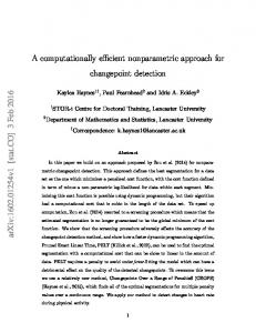
where (ei )i≥1 is the trigonometric basis of X = L2 ([0, 1]) (i.e., e2k−1 = √ √ 2 cos(2πkt), and e2k = 2 sin(2πkt)), and ǫ a Gaussian process independent of P Y with zero mean and covariance operator Γe = j≥1 1j ej ⊗ ej . More precisely, P ǫ was simulated by using a truncation of Γe , Γe (s, t) ≃ qj=1 1j ej (t)ej (s) with q = 500. A sample of size nL = 300 was simulated for training and a sample of size nT = 200 for testing. Figure 1 gives examples of X obtained for model M3 for three different values of y and of the underlying (non noisy) function, F (y)(·). In this example, the simulated data have a high level of noise so that the regression estimation is a rather hard statistical task.

Functional Density-Based Regression

3.2

5

Simulation results

To apply the DBNR method, the discretized functions X were approximated by a continuous function using a functional basis expansion. Specifically, the data were approximated using 128 B-spline basis functions of order 4, as it is shown in Figure 1. The conditional mean µ(·/y) was estimated by a kernel smoothing sample: 44 (Y = 3.7948)

sample: 248 (Y = 1.9879)

sample: 41 (Y = 8.3812) 6

4

4

4 2

0

−2

0

−2

−4

−6

−6 0

0.2

0.4

0.6

0.8

1

argument (t)

0

−2

−4

−4

hal-00658811, version 1 - 11 Jan 2012

functions

2

functions

functions

2

−6 0

0.2

0.4

0.6

0.8

1

0

argument (t)

0.2

0.4 0.6 argument (t)

0.8

1

Fig. 1. True function, F (y)(·) (smooth continuous line), simulated data, X, (gray rough line) and approximation of X using B-splines (rough black line) in M3 for three different values of y

in which the bandwidth parameter h was selected by 10-fold cross-validation minimizing the mean squared error (MSE) criterion. A similar procedure was used to select the parameter p (number of eigenvalues and eigenfunctions used in (3)). Finally, DBNR performance was compared with those obtained by the functional NWK estimate with two kinds of metrics for the kernel: the usual L2 -norm and the PCA based semi-metric norm (see [10] for further details about these methods). The resulting root mean squared errors (RMSE) are presented in Table 1. The results show that DBNR is a good alternative to common NWK Table 1. RMSE for all the methods and all generating models Model M1 M2 M3 M4

FGIR NWK (PCA) NWK (L2 ) 0.08 0.10 0.09 1.47 1.60 1.77 1.79 1.79 2.00 0.94 2.16 1.91

methods. Indeed, DBNR outperforms NWK methods in all the the cases considered in this simulation study that includes both linear (M1) and nonlinear (M2 − M4) models.

6

Hern´ andez et al.

Figures 2 and 3 show how the method performs for each step of the estimation scheme (described in Section 2.2) for the model M3. In particular, Figure 2 gives the result of the first step by displaying the true value and the estimate of F (y)(·) for various values of y (top) and the true value and the estimate of F (·)(t) for various values of t (bottom). The results are very satisfactory given the fact that the data have a high level of noise (which is stressed on in the bottom of the figure): a minor estimation problem appears at the boundaries of F (·)(t), which is a known drawback of the kernel smoothing method. Also, those estimates are smoother than the estimates of F (y)(·): this can be explained by the fact that the kernel estimator is used regarding y and not regarding t, but this aspect can be improved in the future.

Y = 3.7948

Y = 1.9879

Y = 8.3812

3 2

2.5

4

2

3

1

2

1 1

0

µy(t)

µy(t)

µy(t)

0.5 0 −0.5 −1

0 −1

−1 −2

−1.5

−2

−3

−2 −2.5

−3 0

0.2

0.4

0.6

0.8

1

−4 0

0.2

0.4

t

0.6

0.8

1

0

0.2

0.4

t

t = 0.88577

t = 0.12024

4

0

2

−2

10

4 2

0 −2

−4

8

6

µ(y)

2

µ(y)

6

1

8

8

4

0.8

t = 0.41283

10 6

0.6

t

8

µ(y)

hal-00658811, version 1 - 11 Jan 2012

1.5

0 −2

−4 −6

−4

−6

−8

−8

−10

−10

0

2

4

6

Y

8

10

−6 0

2

4

6

Y

8

10

−8

0

2

4

6

Y

Fig. 2. True value (discontinuous lines) and estimate (continuous lines) of F (y)(·) for various values of y (top) and true value and estimate of F (·)(t) for various values of t (bottom) in model M3. The dots (bottom) are the simulated data, X(t).

Figure 3 shows the results of the steps 2-3 of the estimation scheme: the estimated eigendecomposition of r is compared to the true one and finally, the predicted value for Y are compared to the true ones, both on training and test sets. The estimation of the eigendecomposition is, once again very satisfactory given the high level of noise, and the comparison between training and test sets show that the method does not overfit the data.

Functional Density-Based Regression

7

2 1.5

1

1.5 1

1

0.5 0 −0.5

0

−0.5

−1

−1.5

(a) 0

0.2

0.4

0.6

0.8

1

0

0.2

0.4

0.6

0.8

1

0.8 0.6 0.4

10

10

8

8

6 4 2

0.2 0.4

0.6

true eigenvalues

0.8

0.4

1

0.8

1

6 4

(e) 0

0.6

2

(d) 0.2

0.2

t test set (rmse = 1.7952)

predicted Y value

predicted Y value

1

0

(c) 0

t training set (rmse = 1.7184)

1.2

0

−1.5

(b)

t

estimated eigenvalues

0 −0.5

−1

−1 −1.5

hal-00658811, version 1 - 11 Jan 2012

0.5

ψ5(t)

ψ3(t)

ψ1(t)

0.5

0

5

10

(f ) 0

0

true Y values

5

10

true Y values

Fig. 3. Model M3: (a-c)True (dashed line) and estimated eigenfunctions (continuous line), (d) true and estimated eigenvalues and (d-e) predicted vs. true Y values for training and test sets.

4

A study of Tecator dataset

DBNR was also tested on a benchmark data set for functional data: the Tecator dataset6 . It consists in spectrometric data from the food industry. Each of the 215 observations is the near infrared absorbance spectrum of a meat sample recorded on a Tecator Infratec Food and Feed Analyzer. Each spectrum is sampled at 100 wavelengths uniformly spaced in the range 850–1050 nm. The composition of each meat sample is determined by analytic chemistry, so percentages of moisture, fat and protein are associated in this way to each spectrum. This problem is more challenging than the one presented in Section 3 where the data were generated to fulfill exactly the conditions of the DBNR model. The whole data set was randomly split 100 times into training and test sets of almost the same size. The splits were randomly built such that also the training and test set were equally represented over the whole range of fat content. Table 2 reports the mean of the MSE (and its standard deviation) over the 100 divisions both for DBNR and NWK methods. Table 2. Prediction results on Tecator dataset Model DBNR NWK (PCA) NWK (L2 ) MSE 1.91 (0.41) 9.1 (2.1) 8.9 (2.1) 6

Data are available on statlib at http://lib.stat.cmu.edu/datasets/tecator; see [18].

8

Hern´ andez et al.

Results obtained on Tecator by DBNR are the best in the sense of minimum MSE among all the methods. In [10] results based on the use of a semi-metric involving the second order derivatives (which is known to be useful for this data set) were also reported. A MSE of 3.5 was also obtained, which is still larger than the use of DBNR without derivative information.

hal-00658811, version 1 - 11 Jan 2012

5

Conclusions

A new functional nonparametric regression approach has been introduced motivated by the calibration problems in chemometrics. The new method, named functional density-based nonparametric regression (DBNR) was fully described under a Gaussian assumption for the distribution of X given Y but it could be extended to other kinds of distributions. The simulation study and the application of DBNR to a real data set have shown that DBNR performs well and outperforms functional NWK regression methods. Thus, DBNR can be considered a promising alternative to existing functional regression methods, particularly appealing for calibration problems.

References 1. Ramsay, J., Silverman, B.: Functional Data Analysis. Second edn. Springer, New York (2005) 2. Ramsay, J., Dalzell, C.: Some tools for functional data analysis. Journal of the Royal Statistical Society, Series B 53 (1991) 539–572 3. Hastie, T., Mallows, C.: A discussion of a statistical view of some chemometrics regression tools by i. e. frank and j. h. friedman. Technometrics 35 (1993) 140–143 4. Marx, B.D., Eilers, P.H.: Generalized linear regression on sampled signals and curves: a p-spline approach. Technometrics 41 (1999) 1–13 5. Cardot, H., Ferraty, F., Sarda, P.: Functional linear model. Statistics and Probability Letter 45 (1999) 11–22 6. Cardot, H., Ferraty, F., Sarda, P.: Spline estimators for the functional linear model. Statistica Sinica 13 (2003) 571–591 7. Cardot, H., Crambes, C., Kneip, A., Sarda, P.: Smoothing spline estimators in functional linear regression with errors in variables. Comput. Statist. Data Anal. 51 (2007) 4832–4848 8. Crambes, C., Kneip, A., Sarda, P.: Smoothing splines estimators for functional linear regression. The Annals of Statistics (2008) 9. Preda, C., Saporta, G.: Pls regression on stochastic processes. Comput. Statist. Data Anal. 48 (2005) 149–158 10. Ferraty, F., Vieu, P.: Nonparametric Functional Data Analysis: Theory and Practice (Springer Series in Statistics). Springer-Verlag New York, Inc., Secaucus, NJ, USA (2006) 11. Rossi, F., Conan-Guez, B.: Functional multi-layer perceptron: a nonlinear tool for functional data anlysis. Neural Networks 18(1) (2005) 45–60 12. Preda, C.: Regression models for functional data by reproducing kernel hilbert space methods. J. Stat. Plan. Infer. 137 (2007) 829–840

Functional Density-Based Regression

9

hal-00658811, version 1 - 11 Jan 2012

13. Hern´ andez, N., Biscay, R.J., Talavera, I.: Support vector regression methods for functional data. Lecture Notes in Computer Science 4756 (2008) 564–573 14. Li, K.: Sliced inverse regression for dimension reduction. J. Am. Stat. Assoc. 86 (1991) 316–327 15. Dauxois, J., Ferr´e, L., Yao, A.: Un mod`ele semi-param´etrique pour variable al´eatoire hilbertienne. C.R. Acad. Sci. Paris 327(I) (2001) 6947–952 16. Ferr´e, L., Yao, A.: Functional sliced inverse regression analysis. Statistics 37 (2003) 475–488 17. Ferr´e, L., Villa, N.: Multi-layer perceptron with functional inputs : an inverse regression approach. Scandinavian Journal of Statistics 33 (2006) 807–823 18. Thodberg, H.: A review of bayesian neural network with an application to near infrared spectroscopy. IEEE Transaction on Neural Networks 7(1) (1996) 56–72