A functional spiking neuron hardware oriented model - CiteSeerX

A functional spiking neuron hardware oriented model Andres Upegui, Carlos Andrés Peña-Reyes, Eduardo Sanchez Swiss Federal Institute of Technology at Lausanne, Logic Systems Laboratory, 1015 Lausanne, Switzerland [andres.upegui, carlos.pena, eduardo.sanchez]@epfl.ch

Abstract. In this paper we present a functional model of spiking neuron intended for hardware implementation. The model allows the design of speedand/or area-optimized architectures. Some features of biological spiking neurons are abstracted, while preserving the functionality of the network, in order to define an architecture easily implementable in hardware, mainly in field programmable gate arrays (FPGA). The model permits to optimize the architecture following area or speed criteria according to the application. In the same way, several parameters and features are optional, so as to allow more biologically plausible models by increasing the complexity and hardware requirements of the model. We present the results of three example applications performed to verify the computing capabilities of a simple instance of our model.

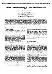
1 Introduction 1.1 Spiking neuron models The human brain contains more than 1011 neurons connected among them in an intricate network. In every volume of cortex, thousands of spikes are emitted each millisecond. Issues like the information contained in these pulses, the code used to transmit information, or the decoding of signals by receptive neurons, have a fundamental importance in the problem of neuronal coding. They are, however, still not fully resolved. ”The neuronal signal consists of short voltage pulses called action potentials or spikes. These pulses travel along the axon and are distributed to several postsynaptic neurons where they evoke postsynaptic potentials. If a postsynaptic neuron receives several spikes from several presynaptic neurons within a short time window, its membrane potential may reach a critical value and an action potential is triggered. This action potential is the output signal which is, in turn, transmitted to other neurons.” [1] Biological neurons are extremely complex biophysical and biochemical entities. Before designing a model it is therefore necessary to develop an intuition for what is important and what can be safely neglected. The Hodgkin-Huxley model [3] describes the generation of action potentials in terms of differential equations resulting on input spike responses as shown in figure 1. In formal spiking neuron models, spikes are fully characterized by their firing time. Typical spiking neuron models as Integrate-

and-fire (I&F) and Spike Response Model (SRM) [1] have been conceived for software implementation, using kernels and numeric integration to represent the neuron response.

Fig. 1. Hodgin-Huxley model response. The neuron receives input spikes at t = 5, 15, 20… 35. The first spike is not strong enough to fire the neuron (i.e. to reach the threshold potential) and generates a postsynaptic response. The spike at time 15 is stronger, and produces a firing; the neuron enters in a refractory period, where the actions of the input spikes are negligible.

1.1 Neural Hardware The inherent parallelism of neural network models has led to the design of a large variety of hardware implementations. Applications as image processing, speech synthesis and analysis, high energy physics, and so on, have found in neural hardware a field with promising solutions. When implemented on hardware, neural networks can take full advantage of their inherent parallelism and run orders of magnitude faster than software simulations becoming thus adequate for real-world applications [2, 4]. While hardware-neural solutions can provide real-time response and learning for networks with large numbers of neurons and synapses, even the fastest sequential processor cannot. Parallel processing with multiple simple processing elements such as SIMD multi-processors provides impressive speedups. Hardware solutions as neurochips (embedded neural units with relatively small complexity, but with high degree of parallelism) obtain largely higher speeds. As parallelism is expensive in terms of chip area, a compromise between speed and cost must be found. Usually, neuron models process, as inputs and outputs, continuous values which are computed using logistic functions [4, 7, 8]. These characteristics lead to more complex models than those of spiking neurons. Spiking-neuron models process discrete values representing the presence or absence of spikes; this fact allows a simpler connectionism structure at the network level, and a striking simplicity at the neuron level as we show in the next section. Implementing models like SRM and I&F on hardware

is largely inefficient, wasting many hardware resources and adding larger delays to implement kernels and numeric integration. This is why a hardware-oriented model is necessary to achieve fast architectures at a reasonable chip area cost.

2 The proposed model Spiking neuron models are characterized by their biological inspiration, relative simplicity, and higher capability of representation compared with traditional models of neurons [4, 7, 8]. They have an inherent capability to represent temporal dynamic patterns due to the information contained in the spike trains frequency and phase. To exploit the coding capabilities of spiking neurons, our model includes, as other standard spiking models do, the following five elements: (1) membrane potential, (2) resting potential, (3) threshold potential, (4) postsynaptic response, and (5) after-spike response (see Figure 2). Each time a pulse, representing a spike, is received by an excitatory (or inhibitory) synapse, the counter that represents the membrane potential is increased (or decreased) a certain value to then decrease (or increase) with a constant slope until the arrival to the resting value. If a pulse arrives when a previous postsynaptic potential is still active, its action is added to the previous one. When the membrane reaches the threshold potential, the neuron fires generating an output spike while its membrane potential goes down to the after-spike potential. After firing, the neuron enters in a refractory period in which it recovers from the after-spike potential to the resting potential. Two kinds of refractoriness are allowed: absolute and partial. Under absolute refractoriness, input spikes are ignored. Under partial refractoriness, the effect of input spikes is attenuated by a constant factor.

Fig. 2. Response of the model to a train of input spikes. The first input spike produces a postsynaptic response. With a train of spikes, the potential grows until it reaches the threshold potential, then the neuron fires and enters a refractory period.

The model is implemented as a Moore finite state machine, a basic hardware description technique to specify the behavior of sequential entities [6]. Two states, op-

erational and refractory, are allowed (see Figure 3). During the operational state, the neuron receives inputs from other neurons. With each input spike the potential increases (excitation) or decreases (inhibition). When the firing condition is fulfilled (i.e., potential ≥ threshold) the neuron fires, the potential takes on the after-spike potential value, and the neuron passes then to the refractory state. The refractory state represents the period required by the neuron to recover from firing. When the membrane potential reaches the resting potential, the neuron passes to the operational state (see Figure 3). As mentioned before, refractoriness can be absolute or partial, depending on whether it takes or not into account new input spikes.

Fig. 3. Finite state machine describing the operation of the neuron. u is the membrane potential, w is the weight of the synapse receiving the spike, k is an attenuation factor, u-rest is the resting potential, thres is the threshold potential, aft_spike is the after-spike potential, and spike-in and spike_out represent respectively the post and pre synaptic events in the neuron. Underlined statements represent conditions, while not underlined represent actions.

For a hardware architecture conception, the neuron would be defined as an embedded processor where the control unit is driven by the finite state machine. The processing unit would be given by a counter with some special features, such as being incremental or decremental at different rates (post-synaptic responses, slopes for operational and refractory states) and it must allow to preset several values (after-spike potential, resting potential).

3 Experimental setup Three experiments have been performed in order to measure the flexibility and the representation power of the model. Our goal was to test the functionality and capabilities of a network of neurons, initially with a static problem (i.e., a XOR gate), then with a simple dynamic problem (i.e., a temporal 3-pattern recognizer), and then with a more-complex dynamic problem (i.e., a temporal 10-pattern number recognizer). A generic network topology is proposed for all the problems (see figure 4). It consists on a network with 3 layers: input, hidden, and output with recurrent connections allowed only on the hidden layer. To provide the input to the network, the logical values '1' and '0' of the patterns are represented, respectively by a train of three spikes and by the absence of spikes. Due to the propagation of spikes throughout the network, the classification spikes arrive a certain time after the presentation of the full pattern.

Fig. 4. Topology of the network for pattern recognition.

The patterns for the temporal pattern recognition problem are: +, × and ◊, drawn on a grid of 5 x 5 pixels (Figure 5). A pattern is presented to the network row after row. The topology of the network consists of an input layer of 5 neurons (one for each column), a recurrent hidden layer with 10 neurons, and an output layer with 3 neurons, one for each pattern (see Figure 4).

Fig. 5. Training patterns. Patterns are presented as the time flows. Each row is presented at a sample period of n iterations.

For the number-recognition problem, the ten numbers are represented with a grid of 4 columns and 5 rows (see Figure 6). The network has 8 input neurons, 30 hidden neurons, and 10 output neurons (we use the negation of the pattern as input, as it increases the amount of useful information). In order to reduce cases where several output neurons fire with the same input, we used a competitive strategy inhibiting reading outputs after a first output fires (i.e., the pattern is considered as classified).

Fig. 6. Number patterns on a grid 4 x 5.

3.1 Genetic weight determination We used a simple genetic algorithm [5] to search for the connection weights. For each problem the basic genome encodes up to three groups of weights: input-to-hidden,

hidden-to-hidden and hidden-to-output (note that hidden-to-hidden weights exist only in recurrent networks). The number of neurons in the involved layers defines thus the number of weights. For the pattern-recognition problem the genome encodes 180 synapse weights taking values from -255 to 256 using 7-bit resolution for a total genome length of 1260 bits. Crossover probability: 0.9, mutation probability: 0.001, 200 individuals and 500 generations. The fitness evaluates the classification error and penalizes high weights values (fitness = 9 - classification error – average normalized weights). The classification error is given by both undesired firing neurons and not-firing neurons expected to do it. For the number-recognition problem the genome encodes, beside the weights, some neuron parameters: the resting potential, the threshold potential and the postsynaptic slope. The weights take on values from -127 to 128 with 6-bit resolution; the potential values go from 0 to 255 with 8-bit resolution, and the slope from 1 to 9 with 3-bit resolution. The total length of the genome is thus 8659 bits. For this latter problem we used a two-stage incremental evolution to search for the solution. The first stage uses an ‘easy’ fitness criterion to perform coarse tuning; its goal is to find several individuals with acceptable performance. The second stage uses a ‘harder’ fitness criterion to finely tune the parameters of a set of the best individuals previously found which are used as initial population. The ‘easy’ fitness computes two scores: the number of patterns correctly classified without considering if the classification was ambiguous or not (see Table 1) and a second score obtained by comparing the non-fired outputs in both the desired and the obtained classification vectors. We refer to it as ‘easy’ because the fitness difference between good individuals is short. The fitness function is given by: fitness = sum (correctly classified patterns) /10 + sum(correctly not classified patterns)/90. The scale factors 1/10 and 1/90 normalize the expression, leading to a maximum fitness of 2. Table 1. Criteria used to describe the quality of classifications.

Criterion Accurate classification Ambiguous classification Undetected pattern Misclassification

Description The desired output vector is obtained (i.e., the classification error is 0) The desired output is activated, but another one fires too. There is no classification.

Output example 100 (desired) 100 (obtained) 100 (desired) 101 (obtained) 100 (desired) 000 (obtained) The pattern is classified in at least one 1 0 0 (desired) wrong class, but not in the desired one. 0 1 0 (obtained)

The ‘harder’ fitness criterion has a more rugged landscape, due to a larger difference between good individuals; it penalizes harder the ambiguous classifications, while the previous strategy was very indulgent with them. The fitness evaluates each pattern and assigns a score according to the percentage of good classifications (1 point), ambiguous classifications (0.5 points), undetected classification (0.5 points), and misclassifications (0 points), and penalizes the number of output spikes generated,

in order to reduce the classification of the same pattern on several classes. The fitness is given by: (accurate classifications x 1) + (ambiguous classifications x 0.5) + (undetected patterns x 0.5) – (total number of fired outputs /50). The maximum fitness, that would be obtained with 10 accurate classifications and 10 fired outputs, values 9.8. Each evolutionary stage was carried out using different parameters. For the first one we used a crossover probability of 0.9, a mutation probability of 0.0001, an elitism of 2, 200 individuals, and 500 generations. For the second one we used a crossover probability of 0.1, a mutation probability of 0.001, an elitism of 1, 10 individuals, and 500 generations. The second one uses atypical values for the probabilities of the genetic operators and for the size of the population since it is intended to perform a mutation-driven tuning for some good individuals.

4 Results Several evolutionary runs were carried out for each genetic algorithm, for the patternrecognition problem the genetic algorithm always finds a solution that classifies correctly the three patterns. The best individual has a fitness of 8.54, it means that the classification error is 0 and the mean of abs(weights) is 117, the minimum value is 255, and the maximum is 248, what lead us to suspect that the weight optimization is not performing very well, the evolution looses easily the best individual, because of that we introduce elitism in the number-recognition problem. For the sensitivity test we found, for 10 runs, an average accurate classification of 170.3 on 300 noisy patterns, 80.2 undetected patterns, 36.7 ambiguous classifications, and 12.8 misclassifications (It has to be considered that the sensitivity test is done on an already trained pattern without any generalization method, and the training does not takes into account any test or validation set). For the number-recognition problem the first stage finds an individual that accurately classifies 3 patterns, the remaining 7 patterns are ambiguously classified. The achieved fitness is 1.844, what means that all patterns are correctly classified due to all expected neurons fired, but there were also 14 not expected output firings (over 100 possible firings). At the second stage, the best individual found using the first criterion exhibits a fitness of 6.02 (3 accurately classified x 1 + 7 ambiguous classification x 0.5 – 24 output spikes / 50). After the fine tuning at the second stage we obtain accurate classification for 6 patterns (1, 3, 4, 6, 7, 0) and undetected pattern for the remaining 4, leading to a fitness of 7.88 (6 accurately classified x 1 + 4 undetected pattern x 0.5 – 6 output spikes / 50). This indicates that the network should not have the complexity required to solve the problem.

5 Conclusions and future work We have presented a functional spiking neuron model suitable for hardware implementation, the proposed model neglects a lot of characteristics from biological and

software oriented models. Nevertheless it keeps its functionality and it is able to solve a relative complex task like temporal pattern recognition. Since the neuron model is highly simplified the lack of representation power of single neurons must be compensated by a higher number of neurons, which in terms of hardware resources could be a reasonable trade-off considering the architectural simplicity allowed by the model. The next step is to design and test a hardware specification using a hardware description language such as VHDL, in order to compare the results with the simulated ones. The model should lead us to neuron architectures with low area requirements. An important issue to consider is the connectionism of the network since its complexity could increase dramatically as the application requires higher number of neurons. Genetic algorithms training have demonstrated to be time consuming on simulations, in addition they require a considerable amount of memory, what makes them inappropriate for a hardware modeling (memory is extremely expensive in hardware applications), so we have to conceive a learning algorithm suitable for this model. The learning algorithm must be suitable for hardware implementation and must have the flexibility to be performed online and onchip, in order to implement it on a field programmable gate array (FPGA). These encouraging results lead us to explore some variations on the model such as inclusion of partial refractoriness and inclusion of differential slopes in order to have a more biologic approach, evaluating the convenience of the trade-off complexity vs functionality. Variations in the search and optimization method should also be considered such as evolution of architectures, mixture of evolution and learning like weight learning with neuron parameters and network architecture evolution.

References 1. W., Kistler W. Spiking neuron models. Cambridge University Press. 2002. 2. Liao Y. Neural networks in hardware: A survey. http://wwwcsif.cs.ucdavis.edu/~liaoy /research/NNhardware.pdf 3. Hodgkin, A. L. and Huxley, A. F. (1952). A quantitative description of ion currents and its applications to conduction and excitation in nerve membranes. J. Physiol. (Lond.), 117:500544 4. Perez-Uribe A. Structure-adaptable digital neural networks. PhD thesis. 1999.EPFL. http://lslwww.epfl.ch/pages/publications/rcnt_theses/perez/PerezU_thesis.pdf 5. Vose M. The Simple Genetic Algorithm: Foundations and Theory 6. Mange D. and Tomassini M. (eds.) Bio-Inspired Computing Machines, Presses Polytechniques et Universitaires Romandes, Lausanne, Switzerland, 1998 7. Hikawa H. Frequency-based multilayer neural network with on-chip learning and enhanced neuron characteristics, IEEE Trans. Neural Networks, 10(3): 545-553, May 1999. 8. Maya S., Reynoso R., Torres C., Arias-Estrada M. Compact Spiking Neural Network Implementation in FPGA, Field Programmable Logic Conference (FPL'2000). Austria. Pages 270-276, 2000.