Hindawi Publishing Corporation Journal of Applied Mathematics Volume 2013, Article ID 986172, 18 pages http://dx.doi.org/10.1155/2013/986172
Research Article A Fuzzy Rule for Improving the Performance of Multiobjective Job Dispatching in a Wafer Fabrication Factory Toly Chen and Yi-Chi Wang Department of Industrial Engineering and Systems Management, Feng Chia University, No. 100, Wenhwa Road, Seatwen, Taichung City 407, Taiwan Correspondence should be addressed to Toly Chen;
[email protected] Received 1 January 2013; Revised 21 August 2013; Accepted 22 August 2013 Academic Editor: Constantinos Siettos Copyright © 2013 T. Chen and Y.-C. Wang. This is an open access article distributed under the Creative Commons Attribution License, which permits unrestricted use, distribution, and reproduction in any medium, provided the original work is properly cited. This paper proposes a fuzzy slack-diversifying fluctuation-smoothing rule to enhance the scheduling performance in a wafer fabrication factory. The proposed rule considers the uncertainty in the remaining cycle time and is aimed at simultaneous improvement of the average cycle time, cycle time standard deviation, the maximum lateness, and number of tardy jobs. Existing publications rarely discusse ways to optimize all of these at the same time. An important input to the proposed rule is the job remaining cycle time. To this end, this paper proposes a self-adjusted fuzzy back propagation network (SA-FBPN) approach to estimate the remaining cycle time of a job. In addition, a systematic procedure is also established, which can solve the problem of slack overlapping in a nonsubjective way and optimize the overall scheduling performance. The simulation study provides evidence that the proposed rule can improve the four performance measures simultaneously.
1. Introduction The task of job dispatching is to determine which jobs must be processed next on the available machines. However, job dispatching in a wafer fabrication factory is a very difficult task. A single recipe may contain more than 500 steps, and a wafer fabrication factory can produce as many as 200 products. In addition, some machines in a wafer fabrication factory, for example, steppers, are very expensive, and there are only a very limited number of them. Therefore, wafers have to revisit these machines for the processing of different layers. This gives rise to the characteristic re-entrant flows. The scheduling of a wafer fabrication factory usually needs to consider various points of view. To shorten the cycle time is one, and to meet the due date is another. However, for such a complex production system, it is difficult to optimize even a single measure [1, 2], let alone the simultaneous optimization of multiple measures. To solve this problem, many attempts have been made in the literature. Some results are as follows. First, a na¨ıve aggregation of single-objective heuristics does not necessarily yield feasible nondominated solutions [3]. In addition, considering the weighted sum
of multiple objectives often leads to unsatisfactory results. Further, scaling parameters can be used to weigh the different objectives, and the determination of appropriate weights is a key research issue. On the other hand, job scheduling in a wafer fabrication factory is subject to many sources of uncertainty or randomness. Such uncertainty or randomness is partly due to manual operations, including loading and unloading jobs, setting up or repairing machines, visual inspection, and others. Other causes include unexpected releases of emergency orders and machine breakdowns that are beyond the control of the factory. To consider the uncertainty or randomness, fuzzy methods are easier to use than probabilistic (stochastic) methods. A fuzzy slack-diversifying fluctuation-smoothing rule is proposed in this study for multiobjective job dispatching in a wafer fabrication factory. The existing fuzzy dispatching rules usually take the form of fuzzy inference rules; for example, “if the total processing time is long and the due date is tight then the job priority is high” [4, 5]. To give a precise schedule, usually multiple fuzzy dispatching rules are used simultaneously. The results of these
2
Journal of Applied Mathematics Table 1: Some existing fuzzy dispatching rules.
References
System type
Rules/inputs/outputs
Xiong et al. [4] Benincasa et al. [5] Lee et al. [9] Tan and Tang [10] Dong and Liu [11]
TSK Mamdani Single-rule-based Mamdani ANFIS
2/2/1 27/3/1 2/4/1 8/4/1 16/4/1
Tsai and Chen [12]
Fusion
4/5/1
∗
Number of objectives 2 (average cycle time, lateness) 2 (average cycle time, WIP level) 2 (average cycle time, cycle time standard deviation) 3 (throughput, average cycle time, no. of vehicles) 1 (average cycle time) 4 (average cycle time, cycle time standard deviation, maximum lateness, number of tardy jobs)
WIP: work-in progress.
dispatching rules must be aggregated. To this end, there are at least three types of fuzzy inference systems—Mamdani’s fuzzy inference systems [6], Takagi-Sugeno-Kang’s (TSK’s) [7] fuzzy inference systems, and adaptive neurofuzzy inference systems (ANFISs) [8]. These systems use different aggregation and defuzzification methods. Xiong et al. [4] scheduled a flexible manufacturing system (FMS) using two fuzzy dispatching rules of the TSK type. Lee et al. [9] established fuzzy inference rules to select a combination of some existing dispatching rules for scheduling a FMS. The effectiveness of a fuzzy inference system depends critically on the way in which the related variables are partitioned. For this reason, Tan and Tang [10] applied Taguchi’s design of experiment (DOE) techniques to improve the design of some fuzzy dispatching rules for a test facility. According to Benincasa et al. [5], up to 27 rules (each with three inputs and one output) were established for scheduling automated guided vehicles. According to Dong and Liu [11], the uncertainty in the processing time was modeled with a fuzzy number, and an ANFIS was established to schedule a job shop. Inputs to the ANFIS were the differences between any two jobs, while the output from the ANFIS determined the sequence of the two jobs. If the output was greater than zero, then the first job should be processed before the second job. Tsai and Chen [12] fuzzified four traditional dispatching rules, and added five adjustable parameters to merge the four rules. A summary of some existing fuzzy dispatching rules is shown in Table 1. The existing approaches have the following problems. (1) Establishing fuzzy inference rules is a subjective process that is not easy to optimize. (2) The fuzziness of parameters causes the uncertainty in scheduling and therefore must be controlled. (3) The parameters that have the greatest relevance for the scheduling performance must be estimated more accurately (such as the remaining cycle time), in order to enhance the effectiveness of scheduling. (4) How to solve ties, that is, jobs with the same slacks, when the parameters are fuzzy valued has not been fully discussed. To tackle these problems and to enhance the performance of multiobjective job scheduling in a wafer fabrication factory, a fuzzy slack-diversifying fluctuation-smoothing rule is proposed in this study. The unique features of the proposed methodology include the following.
(1) Considering the uncertainty in the remaining cycle time. Dispatching rules that consider the remaining cycle time are more able to respond to the changes in the production environment [13]. To consider the uncertainty in the remaining cycle time, it is estimated with a fuzzy number and fed into a fuzzy dispatching rule. To this end, a self-adjusted fuzzy back propagation network (SA-FBPN) approach is proposed. Compared with the existing methods, this SA-FBPN approach can generate a very precise estimate of the remaining cycle time in an efficient manner. (2) Establishing a fuzzy dispatching rule directly from the existing rules. A fuzzy slack-diversifying fluctuationsmoothing rule is proposed by fuzzifying the fourobjective fluctuation-smoothing dispatching rule [14] and diversifying the job slack. This rule accepts the fuzzy remaining cycle time as an input. (3) Diversifying the slack with a new approach: according to Wang et al. [15], the slack was defuzzified by maximizing the standard deviation. However, such a treatment has several drawbacks. This study establishes a systematic procedure to overcome those drawbacks, so that the slacks of jobs can be evenly distributed, and the possibility of forming ties may be reduced as much as possible. (4) Solving the problem of slack overlapping without the need to defuzzify the slacks subjectively. (5) Proposing the fuzzy intersection (FI) and generalized average (GAV) approach to aggregate the estimation results from various FBPNs. Some predictive scheduling methods have been proposed in recent years. The differences between the proposed methodology and these methods were summarized in Table 2. The distinct advantages of the proposed methodology over these predictive scheduling methods include the following. (1) The upper and lower bounds of the remaining cycle time used in the proposed methodology are tighter. (2) The proposed methodology provides an easier way to optimize the scheduling rule, which improves the usability of the proposed methodology. To assess the effectiveness of the proposed methodology, production simulation is also applied in this study. The rest of
Journal of Applied Mathematics
3
Table 2: The differences between the proposed methodology and some predictive methods. Remaining cycle Types of inputs Types of outputs Scheduling method time estimation to the rule from the rule method Tsai and Chen [12]
Number of objectives
Number of adjustable parameters
Effective FBPN
Crisp + fuzzy
Fuzzy
4
5
FCM-FBPN
Crisp
Crisp
2
1
FCM-BPN-GP
Crisp + fuzzy
Fuzzy
2
1
Postclassifying FBPN
Crisp
Crisp
2
2∼3
Chen and Romanowski [23]
FCM-BPN
Crisp
Crisp
2
2
The proposed methodology
SA-FBPNaggregation
Crisp + fuzzy
Fuzzy
4
5
Chen and Wang [21] Chen [22] Chen and Wang [37]
∗
Optimization method Minimizing the sum of the standard deviations of slacks by FNLP Minimizing the standard deviation of slack by polynomial fitting A systematic procedure for diversifying the fuzzy slack Enumeration Minimizing the standard deviation of slack by polynomial fitting A systematic procedure for diversifying the fuzzy slack
FCM: fuzzy c-means; BPN: back propagation network; GP: goal programming; FNLP: fuzzy nonlinear programming.
Table 3: The steps of fabricating a semiconductor product. Step OXWS MKWF ALZER ETZER STZER ALNW
Step no. 1 2 3 4 5 6
QCOG
121
Machine 4HTB, 6HTB, 2DOD, 3DOD, 1WOD, 3WOD, 4WOD, 5WOD 1PFC, 2PFC 7B-I200 1B-DP5KZ 1B-DASP, 3B-DASP, 1B-DULT, 2B-DULT, 9B-DULT, 10B-DULT 10B-I100, 9B-I100, 5B-I200, 7B-I200, 11B-I80 .. . 4HTB, 6HTB, 2DOD, 3DOD, 1WOD, 3WOD, 4WOD, 5WOD
this paper is organized as follows. Section 2 briefly describes the production environment of a wafer fabrication factory. Then, the scheduling problem to be solved is defined. The proposed method for this is described. Section 3 is divided into three parts: SA-FBPN, the fuzzy slack-diversifying fluctuation-smoothing rule, and systematic slack diversification. The SA-FBPN approach is proposed to estimate the remaining cycle time of a job with a fuzzy number. To accept the fuzzy remaining cycle time as an input, the four-objective dispatching rule is fuzzified, resulting in fuzzy-valued slacks that may overlap. In order to solve the problem of slack overlapping, a systematic procedure is established to diversify the slack. In Section 4, a wafer fabrication simulation system is applied to test the effectiveness of the proposed methodology, so that its advantages and disadvantages can be discussed. Finally, some concluding remarks are given in Section 5.
2. Problem Description At a very high level, integrated circuit production may be divided up into five blocks: raw substrate, wafer fabrication, wafer test, mark and final test, and packaging. A wafer
Machine no. 1, 2, 3, 4, 5, 6, 7, 8 9, 10 11 12 13, 14, 15, 16, 17, 18 19, 20, 21, 11, 22 1, 2, 3, 4, 5, 6, 7, 8
fabrication factory is one of the most complex production systems. The complexity of a wafer fabrication process may be characterized by the number of mask layers or major process steps. Inputs to a wafer fabrication factory include 8, 12, or 18 inch wafers, on which various types of integrated circuits can be made. There are four basic steps to fabricate a wafer: film, etching, diffusion, and photo lithography. These steps will be repeated many times; finally a wafer may need to go through hundreds of production steps. In addition, 20 to 30 pieces of wafers are grouped into a job/lot and may be processed together. In total, there may be more than 1000 jobs (or 30000 wafers) that are being processed or to be processed in a wafer fabrication factory. To this end, typically hundreds of machines are used simultaneously in a wafer fabrication factory. In addition, a wafer may visit the same machine multiple times, which constitutes a special type of production system—a re-entrant job shop. An example is given in Table 3. In theory, the problem of scheduling a simple job shop to optimize a single regular measure, for example, 𝐽𝑚 ‖ 𝐶max , is already NP-hard. Scheduling a reentrant job shop to optimize multiple measures at the same time is much more difficult. To tackle such difficulties, the following treatments are taken in this study.
4
Journal of Applied Mathematics Table 4: The nomenclature table.
Variable/parameter
Meaning
𝑡 𝑅𝑗
The current time The release time of job 𝑗; 𝑗 = 1 ∼ 𝑛
CT𝑗 ̃𝑗 CTE
The cycle time of job 𝑗
RCT𝑗𝑢 ̃ 𝑗𝑢 RCTE
The remaining cycle time of job 𝑗 from step 𝑢
RPT𝑗𝑢
The remaining processing time of job 𝑗 from step 𝑢
SCT𝑗𝑢
The step cycle time of job 𝑗 until step 𝑢
SK𝑗𝑢
The slack of job 𝑗 at step 𝑢
𝜆 𝑥𝑗𝑝
Mean release rate The inputs to the three-layer FBPN of job 𝑗, 𝑝 = 1 ∼ 𝑃
ℎ𝑙 𝑤𝑙𝑜
The output from hidden layer node 𝑙, 𝑙 = 1 ∼ 𝐿 The connection weight between hidden layer node 𝑙 and the output node The connection weight between input node p and hidden layer node 𝑙, 𝑝 = 1 ∼ 𝑃; 𝑙=1∼𝐿 The threshold on hidden layer node 𝑙 The threshold on the output node
ℎ 𝑤𝑝𝑙
𝜃𝑙ℎ 𝜃𝑜
The estimated cycle time of job 𝑗 The estimated remaining cycle time of job 𝑗 from step 𝑢
(1) Dispatching rules have often been criticised for being too simple, suboptimal, and myopic. Nevertheless, dispatching rules are still prevalent in the semiconductor manufacturing industry. For this reason, this study aims to propose a new dispatching rule. (2) Predictive information, such as the remaining cycle time estimate, is incorporated into the scheduling rule to improve the responsiveness of the rule to the changing conditions of a wafer fabrication factory. (3) Some of the existing dispatching rules that are effective for four measures (the average cycle time, cycle time standard deviation, the maximum lateness, and the number of tardy jobs) are fused to optimize these measures at the same time. Therefore, the scheduling problem to be investigated can be indicated with 𝐽𝑚 |𝑟𝑗 , 𝑑𝑗 , rent|𝐶, 𝜎𝐶, 𝐿 max , 𝑁𝑇 . A flow chart of the proposed methodology is shown in Figure 1.
3. Methodology The variables and parameters that will be used in the proposed methodology are defined in Table 4. Before any job is scheduled, the remaining cycle time of the job needs to be estimated. To this end, the SAFBPN approach is proposed and the remaining cycle time is estimated with a fuzzy value. 3.1. Step 1: Estimating the Remaining Cycle Time 3.1.1. The SA-FBPN Approach. The remaining cycle time of a job being processed in a wafer fabrication factory is the time still needed to complete the job. The remaining cycle time is
Estimate the remaining cycle time using the SA-FBPN approach
Fuzzify the four-objective fluctuation-smoothing rule
Feed the fuzzy remaining cycle time estimate to the new rule
Establish a systematic procedure to defuzzify the slack
Use the slack-diversifying rule to sequence jobs
Figure 1: The flowchart of the proposed methodology.
an important attribute (or performance measure) for workin-progress (WIP) in a wafer fabrication factory. Past studies (e.g., [14]) have shown that the accuracy of remaining cycle time estimation can be improved by job classification. Soft computing methods (e.g., [16]) have received much attention in this field.
Journal of Applied Mathematics
5
𝐾
𝑛
𝑚 2 𝑒𝑗(𝑘) , Min ∑ ∑ 𝜇𝑗(𝑘) 𝑘=1 𝑗=1
Input layer
1
h w1L
xjP
h wP1
P
w1o w2o
2
Io , ñ o , 𝜃̃o ̃oj
1
···
2
Output layer
I1h , n1h , 𝜃1h , h1
h w11 h w12
1 xj1 xj2
Hidden layer
···
In the SA-FBPN approach, jobs are classified into 𝐾 categories using FCM. First, in order to facilitate the subsequent calculation, all raw data are preprocessed. In the literature, there are two ways of preprocessing. One is partial normalization [17]; the other is variable replacement through principal component analysis (PCA) [18]. However, the simple combination of PCA and FBPN does not have much effect. The main effect of PCA is to improve the correctness of the job classification [19]. Then, we place the (pre-processed) attributes of a job in vector x𝑗 = [𝑥𝑗𝑝 ]; 𝑝 = 1 ∼ 𝑃. FCM classifies jobs by minimizing the following objective function:
aj
wLo
h wP2
h wPL
L ILh , nLh , 𝜃Lh ,
hL
(1) Figure 2: The architecture of the three-layer FBPN.
where 𝐾 is the required number of categories; 𝑛 is the number of jobs; 𝜇𝑗(𝑘) indicates that job 𝑗 belongs to category 𝑘; 𝑒𝑗(𝑘) measures the distance from job 𝑗 to the centroid of category 𝑘; 𝑚 ∈ [1, ∞) is a parameter to adjust the fuzziness and is usually set to 2. The procedure of FCM is as follows. (1) Set 𝐾 = 1.
(6) Calculate the following indexes: 𝐾 𝑛
𝑚 2 𝑒𝑗(𝑘) , 𝐽𝑚 = ∑ ∑𝜇𝑗(𝑘) 𝑘=1𝑗=1
2
2 = min (∑ (𝑥(𝑘1 )𝑝 − 𝑥(𝑘2 )𝑝 ) ) , 𝑒min
(2) Produce a preliminary clustering result.
𝑘1 ≠ 𝑘2
(3) (Iterations) Calculate the centroid of each category as 𝑥(𝑘) = {𝑥(𝑘)𝑝 } ; 𝑥(𝑘)𝑝 = 𝜇𝑗(𝑘) =
𝑝 = 1 ∼ 𝑃,
𝑚 ∑𝑛𝑗=1 𝜇𝑗(𝑘) 𝑥𝑗𝑝 𝑚 ∑𝑛𝑗=1 𝜇𝑗(𝑘)
,
1 2/(𝑚−1)
∑𝐾 𝑞=1 (𝑒𝑗(𝑘) /𝑒𝑗(𝑞) )
,
(2)
2
all 𝑝
(𝑡) where 𝑥(𝑘) is the centroid of category 𝑘. 𝜇𝑗(𝑘) is the membership function that indicates that job 𝑗 belongs to category 𝑘 after the 𝑡th iteration.
(4) Re-measure the distance from each job to the centroid of each category, and then recalculate the corresponding membership. (5) If the following condition is met, go to step (6). Otherwise, return to step (3) as follows: (𝑡) (𝑡−1) < 𝑑, max max 𝜇𝑗(𝑘) − 𝜇𝑗(𝑘) 𝑗
(4)
all 𝑝
𝑆=
𝐽𝑚 . 2 𝑛 × 𝑒min
(7) 𝐾 = 𝐾 + 1. If 𝐾 = 𝐾max , stop; the 𝐾 value minimizing 𝑆 determines the optimal number of categories [20]. Otherwise, return to step (2).
𝑒𝑗(𝑘) = √ ∑ (𝑥𝑗𝑝 − 𝑥(𝑘)𝑝 ) ,
𝑘
RMSE
(3)
where 𝑑 is a real number representing the threshold for the convergence of membership.
After clustering, for each category, a three-layer FBPN is established to estimate the remaining cycle times of jobs in this category. A portion of the jobs is input as the “training examples” to the three-layer FBPN to determine the parameter values. The joint use of fuzzy logic and artificial neural networks is becoming more common in recent years. For example, fuzzy classifiers were applied in [21–23] to separate jobs in a wafer fabrication factory into different clusters before estimating their cycle times using artificial neural networks. Taghadomi-Saberi et al. [24] established an ANFIS to estimate the antioxidant activity and the anthocyanin content at different ripening stages of sweet cherries. Bui et al. [25] also used an ANFIS to determine the landslide susceptibility in the Hoa Binh province of Vietnam. OcampoDuque et al. [26] proposed a fuzzy inference system to compute ecological risk points (ERPs), thereby estimating the changes in water quality over time. The configuration of the three-layer FBPN is as follows (see Figure 2). First, inputs are the 𝑃 parameters of job 𝑗. Subsequently, there is a single hidden layer with 2𝑃 neurons. Finally, the output from the three-layer FBPN is the ̃ 𝑗𝑢 )) of (normalized) remaining cycle time estimate (𝑁(RCTE job 𝑗, where 𝑁() is the normalization function. The procedure for determining the parameter values is now described. Two phases are involved at the training stage.
6
Journal of Applied Mathematics
First, in the forward phase, inputs are multiplied with weights, summed and transferred to the hidden layer. Then, activated signals are output from the hidden layer as ̃ℎ = (ℎ , ℎ , ℎ ) = 𝑙 𝑙1 𝑙2 𝑙3 =(
1
1 ℎ
1 + 𝑒−̃𝑛𝑙
1
1
(5)
, , ), ℎ ℎ ℎ 1 + 𝑒−𝑛𝑙1 1 + 𝑒−𝑛𝑙2 1 + 𝑒−𝑛𝑙3
where ℎ ℎ ℎ , 𝑛𝑙2 , 𝑛𝑙3 ) = 𝐼̃𝑙ℎ (−) 𝜃̃𝑙ℎ 𝑛̃𝑙ℎ = (𝑛𝑙1 ℎ ℎ ℎ ℎ ℎ = (𝐼𝑙1ℎ − 𝜃𝑙3 , 𝐼𝑙2 − 𝜃𝑙2 , 𝐼𝑙3 − 𝜃𝑙1 ),
In this study, the Levenberg-Marquardt algorithm is applied [27]. Subsequently, the upper bound of each parameter (e.g., ℎ ℎ 𝑜 , 𝑤𝑙3 , and 𝜃3𝑜 ) is to be determined, so that the actual 𝑤𝑝𝑙3 , 𝜃𝑙3 value will be less than the upper bound of the network output. Chen and Wang [28] and Chen and Lin [29] have described how a nonlinear programming (NLP) model can be constructed to adjust the connection weights and thresholds in the FBPN. However, the NP problem is not easy to solve. In the proposed methodology, only the threshold on the output node will be adjusted in an iterative way. This way is much simpler and can also achieve good results. Substituting (8) into (7), 𝑜𝑗2 =
ℎ ̃𝑝𝑙 𝐼̃𝑙ℎ = (𝐼𝑙1ℎ , 𝐼𝑙2ℎ , 𝐼𝑙3ℎ ) = ∑ 𝑤 ⋅ 𝑥𝑗𝑝 all 𝑝
(6)
1
1+𝑒
ln (
all 𝑝
where (−) and (×) denote fuzzy subtraction and multiplication, respectively. ̃ℎ values are also transferred to the output layer with the 𝑙 same procedure. Finally, the output of the FBPN is generated as follows:
1 1 1 =( 𝑜 , 𝑜 , 𝑜 ), −𝑛 −𝑛 1 + 𝑒 1 1 + 𝑒 2 1 + 𝑒−𝑛3
1
𝑜
𝑜
1 + 𝑒𝜃2 −𝐼𝑗2
.
(10)
1 𝑜 − 1) = 𝜃2𝑜 − 𝐼𝑗2 . 𝑜𝑗2
(11)
1 − 1) . 𝑜𝑗2
(12)
Assume that the adjustment made to the threshold on the output node is denoted as Δ𝜃𝑜 = 𝜃3𝑜 −𝜃2𝑜 . After adjustment, the output from the new FBPN, 𝑜𝑗3 , determines the upper bound of the remaining cycle time: 𝑜𝑗3 =
(7)
1
𝑜
1 + 𝑒−𝑛𝑗3
,
(13)
where 𝑜 𝑜 𝑜 𝑛𝑗3 = 𝐼𝑗3 − 𝜃3𝑜 = 𝐼𝑗3 − (𝜃2𝑜 + Δ𝜃𝑜 ) .
where
(14)
Substituting (14) into (13),
𝑛̃𝑜 = (𝑛1𝑜 , 𝑛2𝑜 , 𝑛3𝑜 ) = 𝐼̃𝑜 (−) 𝜃̃𝑜
𝑜𝑗3 =
(8)
= (𝐼1𝑜 − 𝜃3𝑜 , 𝐼2𝑜 − 𝜃2𝑜 , 𝐼3𝑜 − 𝜃1𝑜 ) ,
1 𝑜
𝑜
𝑜
1 + 𝑒−(𝐼𝑗3 −𝜃2 −Δ𝜃 )
.
(15)
And substituting (12) into (15),
̃𝑙𝑜 (×) ̃ℎ𝑙 𝐼̃𝑜 = (𝐼1𝑜 , 𝐼2𝑜 , 𝐼3𝑜 ) = ∑ 𝑤 all 𝑙
𝑜𝑗3 =
𝑜 𝑜 𝑜 ≅ (∑ min (𝑤𝑙1 ℎ𝑙1 , 𝑤𝑙3 ℎ𝑙3 ) , ∑ 𝑤𝑙2 ℎ𝑙2 , all 𝑙
1+𝑒
𝑜 = 𝜃2𝑜 − ln ( 𝐼𝑗2
all 𝑝
1 𝑜 1 + 𝑒−̃𝑛
=
So
ℎ ℎ ℎ 𝑥𝑗𝑝 , ∑ max (𝑤𝑝𝑙1 𝑥𝑗𝑝 , 𝑤𝑝𝑙3 𝑥𝑗𝑝 )) , ∑ 𝑤𝑝𝑙2
𝑜̃𝑗 = (𝑜𝑗1 , 𝑜𝑗2 , 𝑜𝑗3 ) =
1
𝑜 −(𝐼𝑗2 −𝜃2𝑜 )
Therefore,
ℎ ℎ = ( ∑ min (𝑤𝑝𝑙1 𝑥𝑗𝑝 , 𝑤𝑝𝑙3 𝑥𝑗𝑝 ) ,
all 𝑝
=
𝑜 −𝑛𝑗2
all 𝑙
(9)
𝑜 𝑜 ℎ𝑙1 , 𝑤𝑙3 ℎ𝑙3 )) . ∑ max (𝑤𝑙1
all 𝑙
Subsequently, in the backward phase, the training of the FBPN is decomposed into three subtasks: determining the center value and upper and lower bounds of the parameters. First, to determine the center of each parameter (such as ℎ ℎ 𝑜 , 𝜃𝑙2 , 𝑤𝑙2 , and 𝜃2𝑜 ), the FBPN is treated as a crisp net𝑤𝑝𝑙2 work. Some algorithms are applicable for this purpose, such as the gradient descent algorithms, the conjugate gradient algorithms, the Levenberg-Marquardt algorithm, and others.
=
1
−(𝜃2𝑜 −ln(1/𝑜𝑗2 −1)−𝜃2𝑜 −Δ𝜃𝑜 )
1+𝑒
1
𝑜
1 + 𝑒ln(1/𝑜𝑗2 −1)+Δ𝜃
=
1 𝑜
1 + 𝑒Δ𝜃 (1/𝑜𝑗2 − 1)
(16) .
Obviously, the maximum of Δ𝜃𝑜 determines the lowest upper bound. Since 𝑜𝑗3 is the upper bound of the remaining cycle time, 𝑜𝑗3 ≥ 𝑁(RCT𝑗𝑢 ), 1
ln(1/𝑜𝑗2 −1)+Δ𝜃𝑜
1+𝑒 Δ𝜃𝑜 ≤ ln (
1 𝑁 (RCT𝑗𝑢 )
≥ 𝑁 (RCT𝑗𝑢 ) ,
− 1) − ln (
1 − 1) . 𝑜𝑗2
(17) (18)
Journal of Applied Mathematics
Actual cycle time
Upper bound 6
⊤
⊥
Upper bound 3 Upper bound 1
⊤
⊤
7
⊤
⊤
⊥
⊤
⊥ ⊥
Upper bound 2 Upper bound 4 Upper bound 5 Actual cycle time
⊥
⊥
Lower bound 6 Lower bound 1 Lower bound 3 Lower bound 2 Lower bound 4 Lower bound 5
⊥ Final result
Figure 4: Iterative reduction of the lower bound. ⊤
Final result
Figure 3: Iterative reduction of the upper bound.
Equation (18) holds for all jobs, so Δ𝜃𝑜 ≤ min (ln ( 𝑗
1 𝑁 (RCT𝑗𝑢 )
− 1) − ln (
1 − 1)) . (19) 𝑜𝑗2
According to (19), the optimal value of Δ𝜃𝑜 should be set to the maximum possible value: Δ𝜃𝑜∗ = min (ln ( 𝑗
1 𝑁 (RCT𝑗𝑢 )
− 1) − ln (
1 − 1)) . 𝑜𝑗2 (20)
The optimization results of the FBPN are dependent on the initial conditions and therefore are different every iteration. Assume that the optimal value of 𝑜𝑗3 in the 𝑡th replication is denoted by 𝑜𝑗3 (𝑡), then after some iterations, 𝑜𝑗3 (all iterations) = min 𝑜𝑗3 (𝑡) . 𝑡
Δ𝜃
1 − 1) − ln ( = max (ln ( − 1)) . 𝑗 𝑜𝑗2 𝑁 (RCT𝑗𝑢 ) (22) 1
Assume that the optimal value of 𝑜𝑗1 in the 𝑡th replication is denoted by 𝑜𝑗1 (𝑡); then, after some iterations, 𝑜𝑗1 (all iterations) = max 𝑜𝑗1 (𝑡) . 𝑡
3.1.2. Considering the Uncertainty in Job Classification. In past studies, the remaining cycle time of a job is usually determined by the FBPN of the cluster with the highest membership. However, that makes fuzzy classification meaningless. To tackle this problem, various treatments have been taken in the literature [30]. Recently, Wu and Chen [31] proposed the GAV approach to aggregate the estimation results from various BPNs, which is modified by incorporating in the concept of FI in this study. Consider ̃ 𝑗𝑢 = ( max (RCTE𝑗𝑢1 (𝑘)) , RCTE
(21)
In this way, the upper bound of the remaining cycle time is decreased gradually (see Figure 3). Another merit of this approach is that it does not rely on the parameters of the FBPN. In a similar way, the lower bound of each parameter (e.g., ℎ ℎ 𝑜 , 𝜃𝑙3 , 𝑤𝑙3 , and 𝜃3𝑜 ) can be determined, so that each actual 𝑤𝑝𝑙1 value will be greater than the lower bound. The optimal value of Δ𝜃𝑜 can be obtained as 𝑜∗
From Figure 5, it can be seen that if only the remaining cycle time is considered, then the sequence should be 3 → 2 → 1. By contrast, the sequence based on imprecise fuzzy remaining cycle time estimates is 3 → 1 → 2. This problem can be solved by increasing the precision of the remaining cycle time estimate, resulting in the correct sequence, 3 → 2 → 1.
(23)
In this way, the upper bound of the remaining cycle time is increased gradually (Figure 4). Δ𝜃𝑜∗ does not rely on the parameters of the FBPN either.
∑𝐾 𝑘=1
√1/𝜇𝑗(𝑘) ⋅ RCTE𝑗𝑢2 (𝑘)
2/(𝑚−1)
∑𝐾 𝑘=1
√1/𝜇𝑗(𝑘)
2/(𝑚−1)
,
(24)
min (RCTE𝑗𝑢3 (𝑘)) ) , ̃ 𝑗𝑢 (𝑘) is the remaining cycle time of job 𝑗 where RCTE estimated by the FBPN of cluster 𝑘. 3.2. The New Rule 3.2.1. Two Basic Fluctuation Smoothing Rules. Lu et al. [13] proposed two fluctuation smoothing rules—the fluctuation smoothing policy for mean cycle time (FSMCT) and the fluctuation smoothing policy for variation of cycle time (FSVCT). FSMCT effectively diminishes the burst of arrivals to all buffers simultaneously, thereby reducing the mean cycle time. On the other hand, FSVCT attempts to make every job equally late or equally early, thereby reducing the standard
8
Journal of Applied Mathematics
Actual remaining cycle time Job no.1 Job no.2
Job no.3
Job no.1
Job no.3 Imprecise fuzzy estimate
Job no.2
Defuzzified imprecise fuzzy estimate
Job no.2 Job no.1 Job no.1
Job no.3
Job no.3 Precise fuzzy estimate
Job no.2
Defuzzified precise fuzzy estimate
Job no.1Job no.2
Job no.3
Figure 5: Precise remaining cycle time estimation eliminates misscheduling.
deviation of lateness. In fluctuation smoothing rules, each job is assigned a slack value, and the processing order of the job is dependent on the slack value: (FSMCT) 𝑗 SK𝑗𝑢 (FSMCT) = − RCTE𝑗𝑢 𝜆
(25)
SK𝑗𝑢 (FSVCT) = 𝑅𝑗 − RCTE𝑗𝑢 .
(26)
(FSVCT)
Jobs with the smallest slack values will be given higher priorities. 3.2.2. Step 2: The Fuzzy Fluctuation-Smoothing Rule. Subsequently, if the remaining cycle time is estimated with a triangular fuzzy number, then we have two fuzzy fluctuation smoothing rules as (fuzzy FSMCT, FFSMCT) ̃ 𝑗𝑢 ̃ 𝑗𝑢 (FSMCT) = 𝑗 − RCTE SK 𝜆
(27)
(fuzzy FSVCT, FFSVCT) ̃ 𝑗𝑢 . ̃ 𝑗𝑢 (FSVCT) = 𝑅𝑗 − RCTE SK
(28)
To determine the sequence of jobs, the fuzzy slacks need to be compared. To this end, various methods have been proposed in the literature, such as the method based on the probability measure [32], the coefficient of variance (CV) index [8], the method considering the area between the centroid and original points [33], and the method based on the fuzzy mean and standard deviation [34]. For a comparison of these methods, refer to Zhu and Xu [34]. In this study, the method based on the fuzzy mean and standard deviation is applied, because it is relatively simple and can yield reasonable comparison results. To put this in context, the following theorems are introduced.
̃= Theorem 1. The fuzzy mean of a triangular fuzzy number 𝐴 − 𝑎, 𝑥 , 𝑥 + 𝑏) is (𝑥0 0 0 𝜇𝐴̃ = 𝑥0 +
𝑏−𝑎 3
(29)
̃ is while the fuzzy standard deviation of 𝐴 𝜎𝐴̃ = √
𝑎2 + 𝑎𝑏 + 𝑏2 . 18
(30)
Proof (see Zhu and Xu [34]). It is, in fact, the center-of-gravity (COG) method. The following definition details the comparison method based on the fuzzy mean and standard deviation. ̃ and 𝐵̃ ∈ 𝐹(𝑅), the Definition 2. For any two fuzzy numbers 𝐴 ̃ ̃ sequence of 𝐴 and 𝐵 can be determined according to their fuzzy means and standard deviations as follows: ̃ ≻ 𝐵; ̃ (1) 𝜇𝐴̃ > 𝜇𝐵̃ if and only if 𝐴 ̃ ≺ 𝐵; ̃ (2) 𝜇𝐴̃ < 𝜇𝐵̃ if and only if 𝐴 (3) if 𝜇𝐴̃ = 𝜇𝐵̃ , then ̃ ≺ 𝐵; ̃ (i) 𝜎𝐴̃ > 𝜎𝐵̃ if and only if 𝐴 ̃ ≻ 𝐵; ̃ (ii) 𝜎 ̃ < 𝜎 ̃ if and only if 𝐴 𝐴
𝐵
̃ = 𝐵. ̃ (iii) 𝜎𝐴̃ = 𝜎𝐵̃ if and only if 𝐴 3.2.3. The Slack-Diversifying Rule. The idea behind the fluctuation smoothing rules is to disperse the arrivals of jobs to a machine, and the tool to control this is the slack value. For this reason, to diversify the slack values of jobs seems to be a
Journal of Applied Mathematics
9
possible way to disperse their arrivals. To this end, Wang et al. [15] maximized the standard deviation of the slack value: 2
𝑁
𝜎SK𝑗𝑢
∑𝑖=1 (SK𝑗𝑢 − SK𝑢 ) =√ . 𝑛−1
(31)
Proof. See the Appendix.
However, to achieve this, the slack formula should contain at least one parameter that is adjustable and differentiable. In addition, Wu and Chen [31] showed that such a treatment may lead to the situation that most slacks concentrate on the two extremes. 3.2.4. Step 3: The Four-Factor Fuzzy Fluctuation-Smoothing Rule. Chen [14] combined four traditional dispatching rulesEDD, critical ratio (CR), FSMCT, and FSVCT and proposed the four-objective dispatching rule. In the four-objective dispatching rule, the slack of job 𝑗 at processing step 𝑢 is defined as SK𝑗𝑢
Theorem 3. The four-objective nonlinear fluctuation smoothing rule is more responsive than the four original rules if 𝑅𝐶𝑇𝐸𝑗𝑢 is large, which is a common phenomenon in a wafer fabrication factory.
If the remaining cycle time is estimated with a triangular fuzzy number, then (34) becomes 𝛽 𝛼 RPT𝑗𝑢 − min𝑗 RPT𝑗𝑢 ̃ 𝑗𝑢 = ( 𝑗 − 1 ) ⋅ ( ) SK 𝑛−1 max𝑗 RPT𝑗𝑢 − min𝑗 RPT𝑗𝑢
⋅(
𝛽 RPT𝑗𝑢 − min𝑗 RPT𝑗𝑢 𝑗−1 𝛼 =( ) ) ⋅( 𝑛−1 max𝑗 RPT𝑗𝑢 − min𝑗 RPT𝑗𝑢
⋅( ⋅(
⋅(
max𝑗 𝑅𝑗 − min𝑗 𝑅𝑗
)
⋅( 𝜂
RCTE𝑗𝑢 − min𝑗 RCTE𝑗𝑢 max𝑗 RCTE𝑗𝑢 − min𝑗 RCTE𝑗𝑢
(32)
max𝑗 SCT𝑗𝑢 − min𝑗 SCT𝑗𝑢
If 𝛼 = 1 then 𝛽, 𝛾, 𝜗 = 0;
̃ 𝑗𝑢 − min𝑗 RCTE ̃ 𝑗𝑢 max𝑗 RCTE
and vice versa
𝛾, 𝜂, 𝜗 = −1,
and vice versa
𝛾, 𝜗 = 1,
SCT𝑗𝑢 − min𝑗 SCT𝑗𝑢 max𝑗 SCT𝑗𝑢 − min𝑗 SCT𝑗𝑢
SK𝑗𝑢1
⋅(
⋅(
Jobs with the smallest slack values will be given higher priorities. There are many possible models that can form the combinations of 𝛼, 𝛽, 𝛾, 𝜂, and 𝜗. For example,
⋅(
𝛼 = 1 − 2𝛽 − 𝛾,
𝛾 = 𝜗 = 𝜂 + 𝛼,
𝑢
SK𝑗𝑢2 = ( 𝑢 ∈ 𝑍+ ;
𝛾 = 𝜗 = (𝜂 + 𝛼) , V = 1, 3, 5, . . . ,
⋅(
(Logarithmic model 1) ln (2 − 2𝛽 − 𝛾) ; ln 2
𝛾=𝜗=
ln (1.5𝜂 + 𝛼 + 2.5) − 1. ln 2 (36)
The values of 𝛼 and 𝛽 are within [0 1].
max𝑗 𝑅𝑗 − min𝑗 𝑅𝑗
𝛾
)
RCTE𝑗𝑢1 − min𝑗 RCTE𝑗𝑢1 max𝑗 RCTE𝑗𝑢3 − min𝑗 RCTE𝑗𝑢1 SCT𝑗𝑢 − min𝑗 SCT𝑗𝑢 max𝑗 SCT𝑗𝑢 − min𝑗 SCT𝑗𝑢
𝜂
(38)
)
𝜗
) ,
𝛽 RPT𝑗𝑢 − min𝑗 RPT𝑗𝑢 𝑗−1 𝛼 ) ) ⋅( 𝑛−1 max𝑗 RPT𝑗𝑢 − min𝑗 RPT𝑗𝑢
(35)
V
𝛼=
𝑅𝑗 − min𝑗 𝑅𝑗
(34)
(Nonlinear model) 𝛼 = (1 − 2𝛽 − 𝛾) ;
𝜗
)
𝛽 RPT𝑗𝑢 − min𝑗 RPT𝑗𝑢 𝑗−1 𝛼 =( ) ) ⋅( 𝑛−1 max𝑗 RPT𝑗𝑢 − min𝑗 RPT𝑗𝑢
and vice versa. (33)
(Linear model)
(37)
)
which is equivalent to
) ,
𝜂 = −1,
then 𝛼, 𝛽 = 0;
𝜂
= (SK𝑗𝑢1 , SK𝑗𝑢2 , SK𝑗𝑢3 )
)
𝜗
SCT𝑗𝑢 − min𝑗 SCT𝑗𝑢
𝛾
)
̃ 𝑗𝑢 ̃ 𝑗𝑢 − min𝑗 RCTE RCTE
⋅(
where, 𝛼, 𝛽, 𝛾, and 𝜂 and are positive real numbers that satisfy the following constraints:
If 𝜂 = 1
max𝑗 𝑅𝑗 − min𝑗 𝑅𝑗
𝛾
𝑅𝑗 − min𝑗 𝑅𝑗
If 𝛽 = 1 then 𝛼 = 0;
𝑅𝑗 − min𝑗 𝑅𝑗
⋅(
⋅(
𝑅𝑗 − min𝑗 𝑅𝑗 max𝑗 𝑅𝑗 − min𝑗 𝑅𝑗
𝛾
)
RCTE𝑗𝑢2 − min𝑗 RCTE𝑗𝑢2 max𝑗 RCTE𝑗𝑢2 − min𝑗 RCTE𝑗𝑢2 SCT𝑗𝑢 − min𝑗 SCT𝑗𝑢 max𝑗 SCT𝑗𝑢 − min𝑗 SCT𝑗𝑢
𝜗
) ,
𝜂
)
(39)
10
Journal of Applied Mathematics Table 5: An example (𝜆 = 1.18).
# 1 2 3 4 5 6 7 8 9 10 11 12 13 14 15 16 17 18 19
𝑅𝑗 102 756 826 652 208 783 800 478 469 699 836 497 596 798 197 804 163 457 523
SK𝑗𝑢3 = (
𝑗 159 37 37 86 55 84 96 52 65 32 85 45 101 34 79 85 78 44 100
SCT𝑗𝑢 881 227 157 331 775 200 183 505 514 284 147 486 387 185 786 179 820 526 460
RPT𝑗𝑢 560 451 489 729 212 816 946 377 446 398 860 353 819 458 297 837 259 324 740
𝛽 RPT𝑗𝑢 − min𝑗 RPT𝑗𝑢 𝑗−1 𝛼 ) ) ⋅( 𝑛−1 max𝑗 RPT𝑗𝑢 − min𝑗 RPT𝑗𝑢
⋅( ⋅(
⋅(
𝑅𝑗 − min𝑗 𝑅𝑗 max𝑗 𝑅𝑗 − min𝑗 𝑅𝑗
max𝑗 RCTE𝑗𝑢3 − min𝑗 RCTE𝑗𝑢1 SCT𝑗𝑢 − min𝑗 SCT𝑗𝑢 max𝑗 SCT𝑗𝑢 − min𝑗 SCT𝑗𝑢
(40)
)
(42)
(6) If ∑𝑛𝑗=1 𝜓(𝑗 − 1, 𝑗) > 𝜓max , update 𝜓max to ∑𝑛𝑗=1 𝜓(𝑗 − 1, 𝑗). (7) If 𝜓max ≥ a threshold, stop; otherwise, return to step (2).
𝜗
) .
This procedure is a polynomial-time algorithm. By repeated applications of this procedure, one obtains an optimal schedule with the fewest overlaps in 𝑂(𝑛2 ) time.
̃ 𝑘𝑢 . ̃ 𝑗𝑢 < SK Job 𝑗 is processed before job 𝑘 if SK 3.2.5. Step 4: The Four-Factor Fuzzy Slack-Diversifying Fluctuation-Smoothing Rule. Wang et al. [15] diversified the slack by maximizing the standard deviation of the slack. However, such a practice causes slacks to concentrate on the two extremes, rather than being evenly dispersed. To solve this problem, the following procedure is established to diversify the slack instead. (1) Set 𝜓max to 0. (2) Vary the values of the five parameters. (3) Sequence the jobs by Definition 2 in ascending order. ̃ (𝑗)𝑢 ’s (4) Calculate the distance of every two adjacent SK as ̃ (𝑗−1)𝑢 , SK ̃ (𝑗)𝑢 ) = SK(𝑗)𝑢1 − SK(𝑗−1)𝑢3 . 𝑑 (SK
SK𝑗𝑢 (FSVCT) −1297 −371 −397 −1170 −322 −1257 −1566 −464 −647 −296 −1315 −386 −1451 −348 −546 −1288 −484 −353 −1328
̃ 𝑗𝑢 ) > 0, ̃ (𝑗−1)𝑢 , SK 1 if 𝑑 (SK 𝜓 (𝑗 − 1, 𝑗) = { 0 otherwise.
) 𝜂
SK𝑗𝑢 (FSMCT) −1264 −1096 −1192 −1749 −483 −1969 −2285 −898 −1061 −968 −2079 −845 −1961 −1117 −676 −2020 −581 −773 −1766
(5) Evaluate whether there is no overlap by
𝛾
RCTE𝑗𝑢3 − min𝑗 RCTE𝑗𝑢1
RCTE𝑗𝑢 1399 1127 1223 1822 530 2040 2366 942 1116 995 2151 883 2047 1146 743 2092 647 810 1851
(41)
3.2.6. Step 5: Applying the New Rule to Sequence Jobs. An example is given in Table 5. The sequencing results by the two traditional fluctuation smoothing rules are FSMCT: 7 → 11 → 16 → 6 → 13 → 19 → 4 → 1 → 3 → 14 → 2 → 9 → 10 → 8 → 12 → 18 → 15 → 17 → 5. FSVCT: 7 → 13 → 19 → 11 → 1 → 16 → 6 → 4 → 9 → 15 → 17 → 8 → 3 → 12 → 2 → 18 → 14 → 5 → 10. Subsequently, if the remaining cycle time is estimated with a fuzzy value instead (see Table 6), then the sequencing results by the two fuzzy fluctuation smoothing rules are FFSMCT: 7 → 11 → 16 → 6 → 13 → 4 → 19 → 1 → 3 → 14 → 2 → 9 → 10 → 8 → 12 → 18 → 15 → 17 → 5.
Journal of Applied Mathematics
11 Table 6: The example with fuzzy remaining cycle times (𝜆 = 1.18).
# 1 2 3 4 5 6 7 8 9 10 11 12 13 14 15 16 17 18 19
𝑅𝑗 102 756 826 652 208 783 800 478 469 699 836 497 596 798 197 804 163 457 523
𝑗 159 37 37 86 55 84 96 52 65 32 85 45 101 34 79 85 78 44 100
SCT𝑗𝑢 881 227 157 331 775 200 183 505 514 284 147 486 387 185 786 179 820 526 460
RPT𝑗𝑢 560 451 489 729 212 816 946 377 446 398 860 353 819 458 297 837 259 324 740
̃ 𝑗𝑢 RCTE (1200, 1399, 1458) (976, 1127, 1176) (1086, 1223, 1299) (1618, 1822, 1976) (455, 530, 557) (1742, 2040, 2158) (2039, 2366, 2549) (848, 942, 992) (992, 1116, 1176) (853, 995, 1031) (1830, 2151, 2311) (794, 883, 918) (1700, 2047, 2170) (975, 1146, 1256) (659, 743, 800) (1819, 2092, 2318) (560, 647, 708) (685, 810, 839) (1547, 1851, 2042)
(1) The slacks obtained by using the proposed methodology are evenly distributed, and there are very little slack overlapping and very few ties. (2) Conversely, the slacks obtained using Wang et al.’s method concentrate on one or two extremes, and there are still some overlaps and ties that cause difficulties in sequencing jobs and may lead to misscheduling. (3) The cumulative fuzziness during the reasoning process of a fuzzy dispatching rule raises the possibility of forming ties. In this regard, the proposed methodology surpasses Wang et al.’s method in reducing the number of ties. The advantage is 83%. (4) In addition, the proposed methodology also achieves a very good performance in reducing the average overlapping. When compared with Wang et al.’s method, the advantage is as high as 98 hours.
1 0.9 0.8 0.7 0.6 0.5 0.4 0.3 0.2 0.1 0
0
0.1
0.2
0.3
0.4
0.5
SK ju
Figure 6: The fuzzy slacks of the 19 jobs after optimization.
𝜇(SK ju )
Obviously, after considering the uncertainty in the remaining cycle time, the sequencing results are different. The four-factor fuzzy slack-diversifying fluctuationsmoothing rule and Wang et al.’s method are also applied to this example. After 50 iterations, the optimal values of the parameters are (𝛼, 𝛽, 𝛾, 𝜂, 𝜗) = (0.4, 0.08, 0.43, 0.43, 0.03) with 𝜓max = 16. That means that 16 out of 19 jobs are not overlapping with their neighbors. The slacks of the jobs are shown in Figure 6. For a comparison, the slacks obtained by using Wang et al.’s method are shown in Figure 7, in which 𝜎SK𝑗𝑢 = 2.68. Obviously, Consider the following.
𝜇(SK ju )
FFSVCT: 7 → 13 → 19 → 16 → 11 → 1 → 6 → 4 → 9 → 15 → 17 → 8 → 3 → 12 → 2 → 14 → 18 → 5 → 10.
̃ 𝑗𝑢 (FFSVCT) SK (−1357, −1297, −1099) (−421, −371, −221) (−474, −397, −261) (−1325, −1170, −967) (−350, −322, −248) (−1376, −1257, −960) (−1750, −1566, −1240) (−515, −464, −371) (−708, −647, −524) (−333, −296, −155) (−1476, −1315, −995) (−422, −386, −298) (−1575, −1451, −1105) (−459, −348, −178) (−604, −546, −463) (−1515, −1288, −1016) (−546, −484, −398) (−383, −353, −229) (−1520, −1328, −1025)
̃ 𝑗𝑢 (FFSMCT) SK (−1324, −1265, −1066) (−1145, −1096, −945) (−1269, −1192, −1055) (−1904, −1750, −1546) (−511, −484, −410) (−2088, −1969, −1671) (−2468, −2285, −1959) (−949, −898, −805) (−1122, −1061, −938) (−1005, −968, −827) (−2240, −2079, −1759) (−881, −845, −757) (−2086, −1962, −1615) (−1228, −1118, −948) (−734, −677, −593) (−2247, −2020, −1748) (−643, −581, −495) (−803, −773, −649) (−1958, −1767, −1463)
1 0.9 0.8 0.7 0.6 0.5 0.4 0.3 0.2 0.1 0
0
2
4
6
8
10
12
14
SK ju
Figure 7: The fuzzy slacks obtained by using Wang et al.’s method.
4. Simulation Study Simulation is widely used to assess the effectiveness of a scheduling policy, especially when the proposed policy and the current practice are very different [35]. A real wafer fabrication factory located in Taichung Scientific Park of Taiwan with a monthly capacity of about 25,000 wafers was
12
Journal of Applied Mathematics Table 7: The performances of various approaches in the average cycle time.
Average cycle time (hrs) FIFO EDD SRPT CR FSMCT FSVCT 4o-SDR The proposed methodology
A (normal) 1254 1094 948 1148 1313 1014 1183 921
A (hot) 400 345 350 355 347 382 347 267
simulated. We used simulation to avoid disturbing the regular operations of the wafer fabrication factory. The goal was to evaluate the effectiveness of the fuzzy slack-diversifying fluctuation-smoothing rule for multiobjective job scheduling in the wafer fabrication factory. The simulation program has been validated by comparing the actual cycle times with the simulated values and verified by analyzing the trace reports. The wafer fabrication factory produces more than 10 types of memory products and has more than 500 workstations for performing single-wafer or batch operations using 58 nm∼ 110 nm technologies. Jobs released into the wafer fabrication factory are assigned three types of priorities, that is, “normal”, “hot”, and “super hot”. Jobs with the highest priorities will be processed first. The large scale and the reentrant process flows of the wafer fabrication factory exacerbate the difficulties of job dispatching. Currently, the longest average cycle time exceeds three months with a variation of more than 300 hours. The wafer fabrication factory is therefore seeking better dispatching rules to replace FIFO and EDD, in order to shorten the average cycle times and ensure on-time delivery to its customers. One hundred replications of the simulation were successively run. The time required for each simulation replication was about 30 minutes on a PC with Intel Dual E2200 2.2 GHz CPUs and 1.99 G RAM. A horizon of twentyfour months was simulated. To assess the effectiveness of the proposed methodology and to make comparison with some existing approaches, seven methods were tested. FIFO, EDD, shortest remaining processing time (SRPT), CR, FSVCT, FSMCT, and the fourobjective slack-diversifying rule (4o-SDR) [14] were applied to schedule the simulated wafer fabrication factory. We collected the data of 1000 jobs, and then we separated the collected data by product types and priorities. Jobs with the highest priorities are processed first. With FIFO, jobs were sequenced on each machine first by their priorities and then by their arrival times at the machine. With EDD, jobs were sequenced first by their priorities and then by their due dates. With SRPT, the remaining processing time of each job was calculated. Then, jobs were sequenced first by their priorities and then by their remaining processing times. With CR, jobs were sequenced first by their priorities, then by their critical ratios. FSMCT and FSVCT used two stages. First, jobs were scheduled using FIFO, in which the remaining cycle times of all jobs were recorded and averaged at each step. Then, FSMCT/FSVCT was applied to schedule
A (super hot) 317 305 308 300 293 315 271 253
B (normal) 1278 1433 1737 1497 1851 1672 1160 811
B (hot) 426 438 457 440 470 475 339 253
the jobs based on the average remaining cycle times obtained earlier. In other words, jobs were sequenced on each machine first by their priorities, then by their slack values. With 4oSDR, the remaining cycle time of a job was estimated using the fuzzy c-means and back propagation network (FCMBPN) approach [28]; it was a crisp value. The five adjustable parameters were set to (𝛼, 𝛽, 𝛾, 𝜂, 𝜗) = (0.6, 0.2, 0, −0.6, 0) after initial scenarios had been examined. In the proposed methodology, the remaining cycle time of a job was estimated using the SA-FBPN approach. The effectiveness of the SAFBPN approach can be seen from Figure 8. The SA-FBPN approach can generate a very precise interval of the remaining cycle time for each job, thereby reducing the risk of misscheduling. In this case, the performance of the effective FBPN approach [12] was close to that of the proposed methodology. Nevertheless, in theory the proposed SA-FBPN approach will outperform the effective FBPN approach because of its iterative nature. By contrast, the FCM-BPN approach does not guarantee that the actual value falls within a distance of three times the root mean squared error (RMSE) from the estimate. The average cycle time, cycle time standard deviation, the number of tardy jobs, and the maximum lateness of all cases were calculated to assess the scheduling performance. The results were summarized in Tables 7, 8, 9, and 10. According to the experimental results, the following points can be made. (1) For the average cycle time, the fuzzy slack-diversifying fluctuation-smoothing rule outperformed the existing approaches. In this respect, FIFO is often a basis for comparison. The most obvious advantage of the fuzzy slack-diversifying fluctuation-smoothing rule over FIFO was about 31%. (2) The fuzzy slack-diversifying fluctuation-smoothing rule also achieved a very good performance in reducing the maximum lateness. When compared with EDD, the advantage was as high as 36% on average. In this regard, the fuzzy slack-diversifying fluctuationsmoothing rule also outperformed 4o-SDR in most cases, which was reasonable due to the uncertainty in the remaining cycle time. (3) In addition, the fuzzy slack-diversifying fluctuationsmoothing rule surpassed the FSVCT policy in reducing cycle time standard deviation. The most obvious
13
1500
1500
1400
1400
1300
1300 Remaining cycle time (hrs)
Remaining cycle time (hrs)
Journal of Applied Mathematics
1200 1100 1000 900
1200 1100 1000 900
800
800
700
700 600
600 0
10
20 Job # (SA-FBPN)
30
0
40
10
20
30
40
Job # (Effective FBPN)
(a)
(b)
1600 1500 Remaining cycle time (hrs)
1400 1300 1200 1100 1000 900 800 700 600 0
10
Center value Actual value
20 30 Job # (FCM-BPN) Upper bound Lower bound
40
(c)
Figure 8: The performances of three approaches in estimating the remaining cycle time.
Table 8: The performances of various approaches in the maximum lateness. The maximum lateness (hrs) FIFO EDD SRPT CR FSMCT FSVCT 4o-SDR The proposed methodology
A (normal) 401 295 584 302 875 706 360 292
A (hot) −122 −181 −142 −159 −165 −112 −152 −143
A (super hot) 164 144 174 138 125 174 118 113
B (normal) 221 336 718 423 856 686 21 23
B (hot) 172 185 194 192 171 260 94 102
14
Journal of Applied Mathematics Table 9: The performances of various approaches in cycle time standard deviation.
Cycle time standard deviation (hrs)
A (normal)
A (hot)
A (super hot)
B (normal)
B (hot)
55 129 248 69 419 280 71 66
24 25 31 29 33 37 41 18
25 22 22 18 16 27 22 25
87 50 106 58 129 201 30 28
51 63 53 53 104 77 29 33
FIFO EDD SRPT CR FSMCT FSVCT 4o-SDR The proposed methodology
Table 10: The performances of various approaches in the number of tardy jobs. Number of tardy jobs FIFO EDD SRPT CR FSMCT FSVCT 4o-SDR The proposed methodology
A (normal)
A (hot)
A (super hot)
B (normal)
B (hot)
79 71 37 79 58 56 79 37
0 0 0 0 0 0 0 0
12 12 12 12 12 12 12 12
16 19 19 19 19 18 19 19
5 5 5 5 5 5 5 5
advantage was 86% when product type B with normal priority was scheduled. The fuzzy slack-diversifying fluctuation-smoothing rule also surpassed 4o-SDR policy in three out of five cases with an average advantage of 8%. (4) In reducing the number of tardy jobs, the proposed methodology outperformed the existing methods in most cases and achieved the best performance when product type A with hot priority was scheduled. (5) As expected, SRPT performed well in reducing the average cycle times, especially for product types with short cycle times (e.g., product A), but gave an exceedingly bad performance with respect to cycle time standard deviation. If the cycle time is long, the remaining cycle time will be much longer than the remaining processing time, which renders SRPT ineffective. SRPT is similar to FSMCT. Both try to make all jobs equally early or late. (6) The performance of EDD was also satisfactory for product types with short cycle times. If the cycle time is long, it is more likely to deviate from the prescribed internal due date, which makes EDD ineffective. This becomes more serious if the percentage of the product type is high in the product mix (e.g., product type A). CR has similar problems. (7) The FCM-BPN approach was also applied to the fuzzy slack-diversifying fluctuation-smoothing rule. Taking product type A (normal priority) as an example,
the results are shown in Table 11. We noticed that with poorer remaining cycle time estimation, the performances of fuzzy slack-diversifying fluctuationsmoothing rule were indeed worsened. However, incorporating the SA-FBPN approach with the fuzzy slack-diversifying fluctuation-smoothing rule could improve the scheduling performance significantly. (8) Wilcoxon signed-rank test [36], a commonly used nonparametric statistical hypothesis test, was used in this study for comparisons of two related samples or repeated measurements on a single sample, to assess whether their population means differed or not. The results were summarized in Table 12. The null hypothesis 𝐻𝑎 was rejected at 𝛼 = 0.025, which showed that the fuzzy slack-diversifying fluctuation-smoothing rule was superior to seven existing approaches in reducing the average cycle time. With regard to the maximum lateness, the advantage of the fuzzy slackdiversifying fluctuation-smoothing rule over FIFO, SRPT, and FSVCT was significant. Similar results could be observed with cycle time standard deviation. However, the advantage of the fuzzy slackdiversifying fluctuation-smoothing rule was not statistically significant for the number of tardy jobs.
5. Conclusions and Directions for Future Research Multiobjective scheduling in a wafer fabrication factory is a challenging but important task. For such a complex
Journal of Applied Mathematics
15
Table 11: The results of applying the FCM-BPN approach to the fuzzy slack-diversifying fluctuation-smoothing rule. Approach FCM-BPN + the proposed rule SA-FBPN + the proposed rule
Average cycle time 958 921
Maximum lateness 307 292
Cycle time standard deviation 70 66
Number of tardy jobs 37 37
Table 12: Results of the Wilcoxon sign-rank test.
FIFO EDD SRPT CR FSMCT FSVCT 4o-SDR ∗
𝐻𝑎0 (the average cycle time) 𝐻𝑏0 (the maximum lateness) 𝐻𝑏0 (cycle time standard deviation) 𝐻𝑏0 (the number of tardy jobs) 2.02∗∗ 2.02∗∗ 1.21 0.54 ∗∗ 2.02 1.21 1.75∗ 1.21 2.02∗∗ 2.02∗∗ 1.75∗ 0.67 2.02∗∗ 1.48 1.48 1.21 2.02∗∗ 1.48 1.75∗ 1.21 2.02∗∗ 2.02∗∗ 2.02∗∗ 0.54 ∗∗ 2.02 −0.13 0.67 1.21
P < 0.05. P < 0.025.
∗∗
production system, to optimize a single objective is tough enough, and to optimize four objectives at the same time is a remarkable challenge. Further, the uncertainty in various production conditions often leads to incorrect scheduling decisions. To deal with these difficulties, the mainstream of research is still the development of dispatching rules through generalization or fusion. For this reason, this study has proposed an effective fuzzy dispatching rule. First, to consider the uncertainty in the fabrication process, the SAFBPN approach has been proposed to estimate the remaining cycle time of a job. Compared to the existing methods, the SA-FBPN approach can generate a very precise estimate of the remaining cycle time in an iterative manner. The FI-GAV approach has also been proposed to aggregate the estimation results from various FBPNs. Subsequently, the fuzzy slackdiversifying fluctuation-smoothing rule has been proposed. The fuzzy remaining cycle time estimate is input to the fuzzy slack-diversifying fluctuation-smoothing rule to derive the job slack. There are five parameters in the fuzzy slackdiversifying fluctuation-smoothing rule that can be adjusted to optimize the rule. To this end, a systematic procedure has been proposed. After a simulation study, we concluded the following points. (1) By considering the uncertainty in the remaining cycle time, four aspects of the scheduling performance— the average cycle time, the maximum lateness, cycle time standard deviation, and the number of tardy jobs—can indeed be simultaneously improved. However, if the estimation accuracy is insufficient, the scheduling process may be misled. (2) The cumulative fuzziness during a fuzzy inference process must be properly dealt with. (3) By tackling slack overlapping in a nonsubjective way, the problem of misscheduling can be effectively
avoided, which augments the performance of the fuzzy slack-diversifying fluctuation-smoothing rule. However, any further assessment of the proposed methodology requires its application to an actual wafer fabrication factory. In addition, different objectives can be fused and fuzzified in the same way. Further, the SA-FBPN approach can be applied to other real production lines in future studies.
Appendix Proof of Theorem 3. First, let us compare the four-objective nonlinear fluctuation smoothing rule and FSMCT. For a fair comparison, the parameters 𝛽, 𝛾, and 𝜗 are set to 0, because the corresponding variables are not considered in FSMCT. When 𝑗/𝜆 increases by 1%, in FSMCT SK𝑗𝑢 is changed by + 1%) (𝑗/𝜆) − RCTE (1 𝑗𝑢 ⋅ 100% − 1 𝑗/𝜆 − RCTE𝑗𝑢 𝑗 𝑗/𝜆 % = %. = 𝑗 − 𝜆 ⋅ RCTE𝑗𝑢 𝑗/𝜆 − RCTE𝑗𝑢
(A.1)
If RCTE𝑗𝑢 is greater than 𝑗/𝜆, then (A.1) becomes 𝑗 𝑗 − 𝜆 ⋅ RCTE % 𝑗𝑢 𝑗 = %. 𝜆 ⋅ RCTE𝑗𝑢 − 𝑗
(A.2)
Conversely, in the four-objective nonlinear fluctuation smoothing rule, SK𝑗𝑢 will be changed by
16
Journal of Applied Mathematics
0 0 (1 + 1%) (𝑗/𝜆) − (1/𝜆) 𝛼 RPT𝑗𝑢 − min𝑗 (RPT𝑗𝑢 ) 𝑅𝑗 − min𝑗 (𝑅𝑗 ) ( ) ⋅( ) ⋅( ) (𝑛/𝜆) − (1/𝜆) max (RPT ) − min (RPT ) max (𝑅 ) − min (𝑅 ) 𝑗 𝑗𝑢 𝑗 𝑗𝑢 𝑗 𝑗 𝑗 𝑗 𝜂 0 RCTE𝑗𝑢 − min𝑗 (RCTE𝑗𝑢 ) SCT𝑗𝑢 − min𝑗 (SCT𝑗𝑢 ) ( ) ⋅( ) max (RCTE ) − min (RCTE ) max (SCT ) − min (SCT ) 𝑗 𝑗𝑢 𝑗 𝑗𝑢 𝑗 𝑗𝑢 𝑗 𝑗𝑢 − 1 ⋅ ⋅ 100% 0 0 𝛼 RPT𝑗𝑢 − min𝑗 (RPT𝑗𝑢 ) 𝑅𝑗 − min𝑗 (𝑅𝑗 ) (𝑗/𝜆) − (1/𝜆) ( ) ⋅( ) ⋅( ) (𝑛/𝜆) − (1/𝜆) max𝑗 (RPT𝑗𝑢 ) − min𝑗 (RPT𝑗𝑢 ) max𝑗 (𝑅𝑗 ) − min𝑗 (𝑅𝑗 ) 𝜂 0 RCTE𝑗𝑢 − min𝑗 (RCTE𝑗𝑢 ) SCT𝑗𝑢 − min𝑗 (SCT𝑗𝑢 ) ⋅( ) ⋅( ) max𝑗 (RCTE𝑗𝑢 ) − min𝑗 (RCTE𝑗𝑢 ) max𝑗 (SCT𝑗𝑢 ) − min𝑗 (SCT𝑗𝑢 )
(A.3)
0.01𝑗 𝛼 = ( ) ⋅ 100% 𝑗 − 1 =(
0.01𝑗 𝛼 ) ⋅ 100% 𝑗−1
1 ≥1 𝛼
0.01𝑗 𝛼 ≥( ) ⋅ (100)𝛼 % 𝑗−1
(A.12)
Acknowledgment (A.5)
This work was supported by the National Science Council of Taiwan.
References
If RCTE𝑗𝑢 is greater than ((𝑗 − 1)𝛼 + 𝑗𝛼 )/𝜆𝑗𝛼−1 , then 𝛼
RCTE𝑗𝑢 ≥
(𝑗 − 1) + 𝑗𝛼 , 𝜆𝑗𝛼−1 𝛼
𝜆𝑗𝛼−1 RCTE𝑗𝑢 ≥ (𝑗 − 1) + 𝑗𝛼 , 𝑗𝛼 𝛼 ⋅ RCTE𝑗𝑢 ≥ (𝑗 − 1) + 𝑗𝛼 , 𝑗 𝑗
𝑗 𝛼 𝑗 ≤( ) 𝜆RCTE𝑗𝑢 − 𝑗 𝑗−1
≥(
which finishes the proof. The comparison between the fourobjective nonlinear fluctuation smoothing rule and the other rules can be done in similar ways.
𝑗 𝛼 ) %. 𝑗−1
𝜆RCTE𝑗𝑢
(A.11)
𝑗
(A.4)
𝛼 0.01𝑗 𝛼 0.01𝑗 𝛼 ) ⋅ 100% = ( ) ⋅ (1001/𝛼 ) % 𝑗−1 𝑗−1
𝜆⋅
𝑗−1 𝛼 ) , 𝑗
−1≥(
𝜆RCTE𝑗𝑢 − 𝑗
Therefore, (A.3) becomes
=(
(A.10)
𝑗
1001/𝛼 ≥ 1001 = 100.
(
𝑗−1 𝛼 ) , 𝑗
𝜆RCTE𝑗𝑢
because 𝑗 ≥ 1. In addition, since 0 ≤ 𝛼 ≤ 1,
≥(
𝑗−1 𝛼 ) + 1, 𝑗
(A.6) (A.7) (A.8) (A.9)
[1] R. M. Dabbas and J. W. Fowler, “A new scheduling approach using combined dispatching criteria in wafer fabs,” IEEE Transactions on Semiconductor Manufacturing, vol. 16, no. 3, pp. 501– 510, 2003. [2] T. C. Chiang, A. C. Huang, and L. C. Fu, “Modeling, scheduling, and performance evaluation for wafer fabrication: a queueing colored petri-net and GA-based approach,” IEEE Transactions on Automation Science and Engineering, vol. 3, no. 3, pp. 330– 337, 2006. [3] C. Grimme and J. Lepping, “Combining basic heuristics for solving multi-objective scheduling problems,” in Proceedings of the IEEE Symposium Series on Computational Intelligence (CISched ’11), pp. 9–16, April 2011. [4] H. Xiong, M. Zhou, and C. N. Manikopoulos, “Scheduling flexible manufacturing systems based on timed petri nets and
Journal of Applied Mathematics
[5]
[6]
[7]
[8]
[9]
[10]
[11]
[12]
[13]
[14]
[15]
[16]
[17]
[18]
[19]
fuzzy dispatching rules,” in Proceedings of the INRIA/IEEE Symposium on Emerging Technologies and Factory Automation, vol. 3, pp. 309–315, October 1995. A. X. Benincasa, O. Morandin Jr., and E. R. R. Kato, “Reactive fuzzy dispatching rule for automated guided vehicles,” in Proceedings of the IEEE International Conference on Systems, Man and Cybernetics, vol. 5, pp. 4375–4380, October 2003. E. H. Mamdani, “Application of fuzzy logic to approximate reasoning using linguist synthesis,” IEEE Transactions on Computers C, vol. 26, no. 12, pp. 1182–1191, 1977. T. Takagi and M. Sugeno, “Fuzzy identification of systems and its applications to modeling and control,” IEEE Transactions on Systems, Man and Cybernetics, vol. 15, no. 1, pp. 116–132, 1985. C. H. Cheng, “A new approach for ranking fuzzy numbers by distance method,” Fuzzy Sets and Systems, vol. 95, no. 3, pp. 307– 317, 1998. K. K. Lee, W. C. Yoon, and D. H. Baek, “Generating interpretable fuzzy rules for adaptive job dispatching,” International Journal of Production Research, vol. 39, no. 5, pp. 1011–1030, 2001. K. K. Tan and K. Z. Tang, “Vehicle dispatching system based on Taguchi-tuned fuzzy rules,” European Journal of Operational Research, vol. 128, no. 3, pp. 545–557, 2001. M. Dong and M. Liu, “An ANFIS-based dispatching rule for complex fuzzy job shop scheduling problem,” in Proceedings of the International Conference on Information Science and Technology (ICIST ’11), pp. 263–266, March 2011. H.-R. Tsai and T. Chen, “A fuzzy nonlinear programming approach for optimizing the performance of a four-objective fluctuation smoothing rule in a wafer fabrication factory,” Journal of Applied Mathematics, vol. 2013, Article ID 720607, 15 pages, 2013. S. C. H. Lu, D. Ramaswamy, and P. R. Kumar, “Efficient scheduling policies to reduce mean and variance of cycle-time in semiconductor manufacturing plants,” IEEE Transactions on Semiconductor Manufacturing, vol. 7, no. 3, pp. 374–388, 1994. T. Chen, “The optimized-rule-fusion and certain-rule-first approach for multi-objective job scheduling in a wafer fabrication factory,” International Journal of Innovative Computing, Information and Control, vol. 9, no. 6, pp. 2283–2302, 2013. Y.-C. Wang, T. Chen, and C.-W. Lin, “A slack-diversifying nonlinear fluctuation smoothing rule for job dispatching in a wafer fabrication factory,” Robotics & Computer Integrated Manufacturing, vol. 29, no. 3, pp. 41–47, 2013. K. Pal and S. K. Pal, “Soft computing methods used for the modelling and optimisation of Gas Metal Arc Welding: a review,” International Journal of Manufacturing Research, vol. 6, no. 1, pp. 15–29, 2011. T. Chen, Y.-C. Wang, and H.-R. Tsai, “Lot cycle time prediction in a ramping-up semiconductor manufacturing factory with a SOM-FBPN-ensemble approach with multiple buckets and partial normalization,” International Journal of Advanced Manufacturing Technology, vol. 42, no. 11-12, pp. 1206–1216, 2009. T. Chen and Y.-C. Wang, “Long-term load forecasting by the collaborative fuzzy-neural approach,” International Journal of Electrical Power and Energy Systems, vol. 43, no. 1, pp. 454–464, 2012. T. Chen and R. Romanowski, “Precise and accurate job cycle time forecasting in a wafer fabrication factory with a fuzzy data mining approach,” Mathematical Problems in Engineering, vol. 2013, Article ID 496826, 14 pages, 2013.
17 [20] X. L. Xie and G. Beni, “A validity measure for fuzzy clustering,” IEEE Transactions on Pattern Analysis and Machine Intelligence, vol. 13, no. 8, pp. 841–847, 1991. [21] T. Chen and Y. C. Wang, “Enhancing scheduling performance for a wafer fabrication factory: the biobjective slack-diversifying nonlinear fluctuation-smoothing rule,” Computational Intelligence and Neuroscience, vol. 2012, Article ID 404806, 12 pages, 2012. [22] T. Chen, “A fuzzy rule for job dispatching in a wafer fabrication factory-a simulation study,” The International Journal of Advanced Manufacturing Technology, vol. 67, no. 1–4, pp. 47–58, 2013. [23] T. Chen and R. Romanowski, “A novel fuzzy-neural slack-diversifying rule based on soft computing applications for job dispatching in a wafer fabrication factory,” Mathematical Problems in Engineering, vol. 2013, Article ID 980984, 15 pages, 2013. [24] S. Taghadomi-Saberi, M. Omid, Z. Emam-Djomeh, and H. Ahmadi, “Evaluating the potential of artificial neural network and neuro-fuzzy techniques for estimating antioxidant activity and anthocyanin content of sweet cherry during ripening by using image processing,” Journal of the Science of Food and Agriculture, 2013. [25] D. T. Bui, B. Pradhan, O. Lofman, I. Revhaug, and O. B. Dick, “Landslide susceptibility mapping at Hoa Binh province (Vietnam) using an adaptive neuro-fuzzy inference system and GIS,” Computers and Geosciences, vol. 45, pp. 199–211, 2012. [26] W. Ocampo-Duque, R. Juraske, V. Kumar, M. Nadal, J. L. Domingo, and M. Schuhmacher, “A concurrent neuro-fuzzy inference system for screening the ecological risk in rivers,” Environmental Science and Pollution Research, vol. 19, no. 4, pp. 983–999, 2012. [27] J. Nocedal and S. J. Wright, Numerical Optimization, Springer, Berlin, Germany, 2006. [28] T. Chen and Y. C. Wang, “Incorporating the FCM-BPN approach with nonlinear programming for internal due date assignment in a wafer fabrication plant,” Robotics and ComputerIntegrated Manufacturing, vol. 26, no. 1, pp. 83–91, 2010. [29] T. Chen and Y.-C. Lin, “A collaborative fuzzy-neural approach for internal due date assignment in a wafer fabrication plant,” International Journal of Innovative Computing, Information and Control, vol. 7, no. 9, pp. 5193–5210, 2011. [30] T. Chen, “Incorporating fuzzy c-means and a back-propagation network ensemble to job completion time prediction in a semiconductor fabrication factory,” Fuzzy Sets and Systems, vol. 158, no. 19, pp. 2153–2168, 2007. [31] H.-C. Wu and T. Chen, “A fuzzy-neural ensemble and geometric rule fusion approach for scheduling a wafer fabrication factory,” Mathematical Problems in Engineering, vol. 2013, Article ID 956978, 14 pages, 2013. [32] E. S. Lee and R.-J. Li, “Comparison of fuzzy numbers based on the probability measure of fuzzy events,” Computers and Mathematics with Applications, vol. 15, no. 10, pp. 887–896, 1988. [33] T. Chu and C. Tsao, “Ranking fuzzy numbers with an area between the centroid point and original point,” Computers and Mathematics with Applications, vol. 43, no. 1-2, pp. 111–117, 2002. [34] L. Zhu and R. Xu, “Ranking fuzzy numbers based on fuzzy mean and standard deviation,” in Proceedings of the 8th International Conference on Fuzzy Systems and Knowledge Discovery (FSKD ’11), pp. 854–857, July 2011. [35] T. Chen, “A flexible way of modelling the long-term cost competitiveness of a semiconductor product,” Robotics & Computer Integrated Manufacturing, vol. 29, no. 3, pp. 31–40, 2013.
18 [36] F. Wilcoxon, “Individual comparisons by ranking methods,” Biometrics Bulletin, vol. 1, no. 6, pp. 80–83, 1945. [37] T. Chen and Y.-C. Wang, “A post-classifying fuzzy-neural and data-fusion rule for job scheduling in a wafer fab-a simulation study,” International Journal of Manufacturing Research, vol. 8, no. 2, pp. 150–170, 2013.
Journal of Applied Mathematics
Advances in
Operations Research Hindawi Publishing Corporation http://www.hindawi.com
Volume 2014
Advances in
Decision Sciences Hindawi Publishing Corporation http://www.hindawi.com
Volume 2014
Journal of
Applied Mathematics
Algebra
Hindawi Publishing Corporation http://www.hindawi.com
Hindawi Publishing Corporation http://www.hindawi.com
Volume 2014
Journal of
Probability and Statistics Volume 2014
The Scientific World Journal Hindawi Publishing Corporation http://www.hindawi.com
Hindawi Publishing Corporation http://www.hindawi.com
Volume 2014
International Journal of
Differential Equations Hindawi Publishing Corporation http://www.hindawi.com
Volume 2014
Volume 2014
Submit your manuscripts at http://www.hindawi.com International Journal of
Advances in
Combinatorics Hindawi Publishing Corporation http://www.hindawi.com
Mathematical Physics Hindawi Publishing Corporation http://www.hindawi.com
Volume 2014
Journal of
Complex Analysis Hindawi Publishing Corporation http://www.hindawi.com
Volume 2014
International Journal of Mathematics and Mathematical Sciences
Mathematical Problems in Engineering
Journal of
Mathematics Hindawi Publishing Corporation http://www.hindawi.com
Volume 2014
Hindawi Publishing Corporation http://www.hindawi.com
Volume 2014
Volume 2014
Hindawi Publishing Corporation http://www.hindawi.com
Volume 2014
Discrete Mathematics
Journal of
Volume 2014
Hindawi Publishing Corporation http://www.hindawi.com
Discrete Dynamics in Nature and Society
Journal of
Function Spaces Hindawi Publishing Corporation http://www.hindawi.com
Abstract and Applied Analysis
Volume 2014
Hindawi Publishing Corporation http://www.hindawi.com
Volume 2014
Hindawi Publishing Corporation http://www.hindawi.com
Volume 2014
International Journal of
Journal of
Stochastic Analysis
Optimization
Hindawi Publishing Corporation http://www.hindawi.com
Hindawi Publishing Corporation http://www.hindawi.com
Volume 2014
Volume 2014