A Fuzzy Sets Theoretic Approach to Approximate ... - Semantic Scholar

A Fuzzy Sets Theoretic Approach to Approximate Spatial Reasoning ∗† Yongming Lia ‡, Sanjiang Lib a Institute

§

of Fuzzy systems, College of Mathematics and Information Sciences, Shaanxi Normal University, Xi’an, 710062, China;

b State

Key Laboratory of Intelligent Technology and Systems,

Department of Computer Science and Technology, Tsinghua University, Beijing 100084, China.

Abstract Relational composition-based reasoning has become the most prevalent method for qualitative reasoning since Allen’s 1983 work on temporal intervals. Underlying this reasoning technique is the concept of a Jointly Exhaustive and Pairwise Disjoint (JEPD) set of relations. Systems of relations such as RCC5 and RCC8 were originally developed for ideal regions, not subject to imperfections such as vagueness or fuzziness which are found in many applications in geographic analysis and image understanding. This paper, however, presents a general method for classifying binary topological relations involving fuzzy regions using the RCC5 or the RCC8 theory. Our approach is based on fuzzy set theory and the theory of consonant random set. Some complete classifications of topological relations between fuzzy regions are also given. Furthermore, two composition operators on spatial relations between fuzzy regions are introduced in this paper. These composition operators provide reasonable relational composition-based reasoning engine for spatial reasoning involving fuzzy regions. Keywords: Spatial relation, Region Connection Calculus, Relational composition, Consonant random set, Mode, Fuzzy region, Fuzzy logic.

1

Introduction

Originating in Allen’s analysis of temporal relations [1], relational composition has become a key technique in providing an efficient inference mechanism for a wide class ∗

IEEE Transactions on Fuzzy Systems, 2004, 12(6), 745-754. This work was supported by National Science Foundation of China (Grant No: 60174016,10226023), “TRAPOYT” of China and the Key Project of Fundamental Research (Grant No: 2002CB312200). The second author is also supported by NSF of China (Grant No: 60305005). ‡ Email: [email protected] § Email: [email protected] †

1

of theories [1, 19, 30, 29, 32, 31, 13, 14, 8, 25, 26]. This is especially the case for the two closely related fields of Geographic Information Systems (GIS) and Qualitative Spatial Reasoning (QSR). Usually such a technique is based on a well-defined Jointly Exhaustive and Pairwise Disjoint set of relations on the domain of discourse. Suppose D is the domain of discourse, and R = {R1 , · · · , Rn } is a set of binary relations on D. We say R is Jointly Exhaustive and Pairwise Disjoint (JEPD for short) provided that any two elements in D stand to each other in exactly one of these relations. For two relations Ri , Rj in R, the composition of Ri and Rj , denoted by Rij , is defined to be the subset of R such that Rk ∈ Rij if and only if (∃a, b, c ∈ D)[Rk (a, c)∧Ri (a, b)∧Rj (b, c)]. This ensures that whenever Ri (a, b) and Rj (b, c) hold, a and c must be related by some relation symbol Rk in Rij . In practice, the JEPD set of relations is finite and we often summarize the composition results in an n × n table, called the composition table (CT for short). Such a table enables one to answer the following query by a simple table lookup: Given two relational facts Ri (a, b) and Rj (b, c) hold, what are the possible relations that can hold between a and c? This kind of computation is very useful in, e.g., checking the integrity of a large database. This paper is mainly concerned with two most important composition tables of spatial relations, known as respectively the RCC5 CT and the RCC8 CT in the literature. These two tables are respectively based on two sets of JEPD relations known as RCC5 and RCC8 which are defined in the Region Connection Calculus (RCC) [30, 11, 8]. RCC8 is a refinement of RCC5 and hence the RCC5 CT can be easily obtained from the RCC8 CT by relation-algebraic methods. It is widely recognized that RCC8 is an interesting calculus for QSR and GIS research which is worth being studied in detail (see [31] and references therein). Although the work on RCC as well as similar formalisms provides a valuable foundation for QSR and GIS, its basis in crisp regions is a severe limitation for many practical applications in spatial databases and GIS. Recently, researchers are beginning to realize that the feature of spatial vagueness or spatial indeterminacy is inherent to many geographic data (see [5] and references therein). In deed, nearly every geographic region (e.g. mountains, seas, forests, deserts or the downtown of cities etc.) has an indeterminate boundary. Due to the important role of vague objects, there have been considerable research efforts concerned with the classification, modelling and formal characterization of vague geographic data in the literature of spatial analysis and GIS [10, 24, 2, 36, 4, 12, 23, 37, 35, 22]. As far as the formalization of spatial relations between vague regions is concerned, there are also some notable efforts devoted to this topic [6, 9, 34, 39, 3, 20]. The accounts of Cohn and Gotts [9] and Clementini and Di Felice [6] focus on topological or mereological relations and give similar JEPD sets of binary relations between regions with indeterminate boundary. Cohn and Gotts [9] modify the RCC5 theory, the mereological fragment of the RCC theory, whereas Clementini and di Felice [6] take up the 9-Intersection Model of Egenhofer and Herring [18]. Their approaches, however, either represent a vague region simply as a pair of crisp regions or treat the indeterminate boundary of a vague region as a thick boundary. As a consequence finer distinctions between points lying within the thick boundary cannot be made in these approaches. Moreover, since the two JEPD sets identified in [9] and [6] contain 46 and 44 binary relations respectively, the work 2

of building the corresponding composition table is arduous and error-prone. This is even worse when we extend the egg-yolk approach by representing a vague region as, for example, a triple of crisp regions. Indeed, it is in general a considerable challenge for the QSR community to develop such a composition table automatically [29, 7]. The goal of the present paper is to present a more general method for representing and reasoning about topological information among fuzzy regions. This new method is based on the RCC theory and fuzzy set theory. To develop such a theory, firstly we need to establish a formalization of fuzzy regions. In the literature fuzzy regions are usually defined as fuzzy subsets of a referential set in a domain under consideration, obtained by assigning to points (pixels) membership values belong to [0, 1] ([38, 40, 24, 12, 2, 23, 36, 4]). In this paper we are mainly concerned with regions in the Euclidean plane R2 and a crisp region is just a non-empty regular closed set ([21]) in R2 . A fuzzy region is then defined to be a fuzzy set R2 → [0, 1] whose α-cuts and support are proper crisp regions. Since in practice the value sets of fuzzy regions are usually finite, we can assume that the value set of fuzzy regions is a finite set V and write the set of all V -valued fuzzy regions as R(V ). Note that a V -valued fuzzy region A is indeed (uniquely determined by) a consonant random set (See Section 3 of this paper). In other words, a V -valued fuzzy region is just a set of weighted crisp regions. Modelling fuzzy region like this bears similarity to the theory of supervaluation where a vague predicate is assumed to have several equally good interpretations and, correspondingly, a vague region is non-discriminately represented by several crisp regions [22]. The difference is that different crisp interpretations of the same fuzzy region in our case may have different weights. Secondly, fix a finite value set V , we should give a complete classification of binary topological relations between V -valued fuzzy regions. In an early paper, Dubois and Jaulent [15] proposed a general model of spatial relations between fuzzy regions which encompasses specific suggestions made by Rosenfeld [33]. Generally speaking, for any binary predicate R on crisp regions and any two fuzzy regions A, B, this approach associate for the pair (A, B) a value in [0,1] which is calculated as a mathematical expectation based on a probability density function. Recently, this proposal was adopted by Zhan [39] for approximately analyzing binary topological relations between simple fuzzy regions. But as remarked by Roy and Stell [34], Zhan’s approach did not get a JEPD (Jointly Exhaustive and Pairwise Disjoint) set of relations on fuzzy regions. Assume we have in advance a JEPD set R of topological relations on the crisp regions which can be either RCC5 or RCC8. To obtain a JEPD set of relations between fuzzy regions, we suggest to encode the base JEPD relations as canonical unit vectors in the l-dimensional Euclidean cube [0, 1]l (l = 5, 8). Now we can obtain such a JEPD set by adapting Dubois and Jaulent’s method given in [15]. Using the α-cut approach advocated by Krishnapuram, Keller and Ma [23] also yields another scheme of JEPD set of relations on fuzzy regions. Finally, due to the enormous number of base relations in the previously constructed JEPD set between fuzzy regions, the work of developing a composition table based on such a JEPD set is indeed tremendous. Noticing the fundamental role of relational composition in spatial reasoning, however, it is a natural demand to provide a reasonable relational composition-based reasoning engine for fuzzy spa3

tial reasoning. This article also makes a modest attempt to answer this problem. Indeed we propose two composition operators for spatial relations between fuzzy regions based on compositions of the RCC5 and RCC8 relations. The work of Roy and Stell [34], Bittner and Stell [3] also provide methods for extending the RCC relations from crisp regions to indeterminate regions based on rough set ([28]). In a recent paper, Guesgen [20] proposes a method for fuzzifying spatial relations. His approach, however, starting with Allen’s 13 temporal relations, is based on the concept of conceptual neighborhood [19]. The relations obtained are, unlike ours, indeed fuzzy relations. This approach can be seen as orthogonal to ours. The rest of the paper is arranged as follows. First we briefly recall the RCC5 and RCC8 theories for crisp spatial regions and the egg-yolk calculus for regions with indeterminate boundaries. Section 3 introduces our interpretation of vague regions based on fuzzy logic and random set theory, and considers its relation to the interpretation based on the theory of supervaluation. Section 4 proposes a more general method for classifying binary topological relations between fuzzy regions. Some examples of JEPD relations sets involving fuzzy regions based on the RCC5 and RCC8 theories are also given in this section. In section 5, we give two composition operators for spatial relations involving fuzzy regions and some relation-algebraic aspects of these relations are discussed. Conclusions are given in Section 6.

2

The Region Connection Calculus

The Region Connection Calculus (RCC) [30, 29, 11, 8] is a first order theory based on a primitive connectedness relation, C(x, y). RCC is intended to provide a logical framework for incorporating spatial reasoning into AI systems. It is already well known that connected regular topological spaces provide models of the RCC theory. In this paper we only consider the special RCC model constructed from the Euclidean plane R2 . For this model, the domain of possible regions is just the set of non-empty regular closed subsets of R2 ; two regions are said to be connected if they have common points. Using C(x, y), a basic set of binary relations is defined. Definitions and intended meanings of those used here are given in Table 1. The relations P, PP, TPP and NTPP, are non-symmetrical and, therefore, admit inverses. For the inverses we use the notation Φ∼ , where Φ ∈ {P, PP, TPP, NTPP}. The inverse relation Φ∼ is defined by Φ∼ (x, y) iff Φ(y, x). Of the defined relations, there are two important systems of JEPD relations: the RCC5 relations {DR, PO, EQ, PP, PP∼ } and the RCC8 relations {DC, EC, PO, EQ, TPP, NTPP, TPP∼ , NTPP∼ }. Tables 2 gives the RCC5 CT, and, for the RCC8 CT, we refer the reader to [11, 31]. In many cases, the composition of two relations is a disjunction of relations. For more details of the RCC theory we invite the readers to consult the monograph of Renz [31]. The RCC theory was originally developed for ideal regions, thus not subject to imperfections such as vagueness or indeterminacy. Cohn and Gotts [9] propose an extension of the RCC theory, known as egg-yolk theory, to representing and reasoning about spatial regions with indeterminate boundaries. In this theory, a region with indeterminate boundary is modelled by an inner subregion (the yolk ), an outer subregion (the white), and their union (the egg). Then 46 different configurations 4

Table 1: Some relations definable in terms of C (taken from [8]) Relation DC(x, y) P(x, y) PP(x, y) EQ(x, y) O(x, y) PO(x, y) EC(x, y)

interpretation x is disconnected from y x is a part of y x is a proper part of y x is identical with y x overlaps y x partially overlaps y x is externally connected to y DR(x, y) x is discrete from y TPP(x, y) x is a tangential proper part of y NTPP(x, y) x is a non-tangential proper part of y

Definition of R(x, y) ¬C(x, y) ∀z[C(z, x) → C(z, y)] P(x, y) & ¬P(y, x) P(x, y) & P(y, x) ∃z[P(z, x) & P(z, y)] O(x, y) & ¬P(x, y) & ¬P(y, x) C(x, y) & ¬O(x, y) ¬O(x, y) PP(x, y) & ∃z[EC(z, x) & EC(z, y)]. PP(x, y) & ¬∃z[EC(z, x) & EC(z, y)]

Table 2: Composition table for the RCC5 relations. ◦ EQ PP PP∼

EQ

PP∼

PP

∼

PO

DR

EQ

PP

PP

PO

DR

PP

PP

>

PP, PO, DR

DR

∼

∼

PP

PP , PO

PP∼ , PO, DR

PP, PO

PP∼ , PO, DR

>

PP∼ , PO, DR

PP, PO, DR

DR

PP, PO, DR

>

PP

EQ, PP, PP ,

PO DR

∼

∼

PO

PO DR

of topological relations between regions with indeterminate boundaries are classified according to the RCC5 relations holding between the pairs egg-egg, egg-yolk, yolkegg, and yolk-yolk. Since their approach represents a vague region simply as a pair of crisp regions, finer distinctions between points lying within the thick boundary cannot be made. We still need a more general method to cope with topological relations between vague regions. One possible approach was already hinted in [9], where they suggest “using two (or possibly more) concentric subregions, indicating degrees of ‘membership’ in a vague region.” This approach is indeed what the theory of supervaluation suggests. We shall return to this topic later in Section 3.

3

The representation of fuzzy regions

The aim of this section is to develop and formalize the concept of a fuzzy region. Our definition, unlike that of Zhan [39] which is based on the 9-Intersection Model, is based on the RCC theory and the theory of consonant random set.

3.1

Finite valued fuzzy sets and consonant random sets

In general, a fuzzy set A on a referential set Ω is defined as a membership function µA : Ω → [0, 1] which assigns to each x ∈ Ω its membership grade µA (x). We recall 5

some basic concepts about fuzzy set. We call S(A) = {x : µA (x) > 0} the support of A and I(A) = {x : µA (x) = 1} the core of A. For α ∈ [0, 1], the α-cut of A is the crisp set Aα = {x : µA (x) ≥ α}. Note that the set of α-cuts are nested in the sense that α1 ≥ α2 ⇒ Aα1 ⊆ Aα2 . The membership function can be recovered from the set of α-cuts via the representation theorem as follows µA (x) = sup{α : x ∈ Aα }. In practice, the value range of a fuzzy set is usually finite. We call such a fuzzy set a finite valued fuzzy set. A finite valued fuzzy set can be uniquely determined by a consonant random set. This result was first obtained in [16]. For the convenience of the reader, we make a brief introduction here. Recall that a consonant random set is a pair (F, m), where F is a nested family of sets A1 ⊂ A2 ⊂ · · · ⊂ An and m is a basic probability assignment with Σni=1 m(An ) = 1 and m(Ai ) > 0 for each i = 1, · · · , n. On one hand, for a finite valued fuzzy set A represented by µA : Ω → [0, 1], suppose its non-zero membership values is 1 = α1 > α2 > · · · > αn > 0 and assume αn+1 = 0. Set Ai = Aαi and m(Ai ) = αi − αi+1 for i = 1, · · · , n. Then (FA , m) is a consonant random set, where FA = {Ai : i = 1, · · · , n} is clearly a nested family of sets. Given two finite valued fuzzy sets A, B and suppose their corresponding consonant random sets coincide. Then it’s straightforward to prove that A is identical with B. On the other hand, given a consonant random P set (F, m), we can construct a finite valued fuzzy set A as follows: µA (x) = {m(Ai ) : x ∈ Ai ∈ F}. This construction is also one-to-one. We omit the proof here.

3.2

Fuzzy regions and supervaluation

Note that in this paper we are mainly concerned with regions in the Euclidean plane R2 . In the rest of this paper we take Ω = R2 . Recall that in the RCC theory, a (crisp) region is just a non-empty regular closed subset of R2 . We denote this domain of regions by C. A fuzzy region A is a fuzzy set µA : R2 → [0, 1] which satisfies the following condition: (∃u, v ∈ R2 )(µA (u) = 0 & µA (v) = 1) & (∀α ∈ (0, 1])(Aα ∈ C) & S(A) ∈ C. This requires all α-cuts as well as the support of a fuzzy region is a nonempty proper regular closed subset of R2 and hence more general than the concept of simple fuzzy region given in [39], where Zhan requires that the α-cuts are all connected. Since the value set of a fuzzy region is usually finite in practice, we suppose that the set of non-zero values of fuzzy regions is V = {α1 , α2 , · · · , αn } with the orders 1 = α1 > α2 > · · · > αn > 0 in the following. The set of all V -valued fuzzy regions is denoted by R(V ). Write αn+1 = 0. By the result obtained in Section 3.1, we know R(V ) is just the collection of all consonant random sets (F, m) satisfying the following conditions: F = {A1 , · · · , An }, ∅ 6= A1 ⊂ A2 ⊂ · · · ⊂ An 6= Ω, m(Ai ) = αi − αi+1 (i = 1, · · · , n). In this case, the basic probability assignment m(Ai ) can be interpreted [15] to be the probability that Ai is the true representation of A, the fuzzy region. The above random set representation of a fuzzy region bears similarity to Kulik’s geometric theory ([22]) of vague boundaries based on supervaluation. In the theory 6

of supervaluation, a vague predicate is assumed to have several equally good interpretations and, correspondingly, a vague region is non-discriminately represented by several crisp regions. Roughly speaking, a vague region V is just a special consonant random set (F, m) with the following form: F = {A1 , · · · , An }, A1 ⊂ A2 ⊂ · · · ⊂ An , m(Ai ) = 1/n (i = 1, · · · , n). Consequently, our interpretation of fuzzy regions based on the theory of consonant random set is more general than that one based on supervaluation given by Kulik in [22].

4

Spatial relations between fuzzy regions

In this section, we shall propose a general approach for classifying topological relations involving fuzzy regions. In general, given a binary relation between crisp regions, there are two main schemes which can be used to approximate the corresponding relation between two fuzzy regions. To begin with, we view a binary relation R as a function fR : C × C → {0, 1} taking a pair of crisp regions (a, b) to either 1 or 0 depending whether R(a, b) holds, where C is the domain of crisp regions. This function can be generalized to cope with fuzzy regions such that a pair of fuzzy regions A, B is associated with a real number from [0,1] indicating to what extent “A is related to B by R”. Now suppose A, B are two V -valued fuzzy regions, where V = {α1 , · · · , αn } and 1 = α1 > α2 > · · · > αn > 0 = αn+1 . In the first scheme, Dubois and Jaulent [15] suggest that, firstly, we compute the value of fR (Aαi , Bαj ) for all pairs of level sets Aαi and Bαj , and then the overall membership for fR (A, B) is computed as the expected value of the relation via the equation Pn Pn FR (A, B) = j=1 m(Ai )m(Bj )fR (Ai , Bj ) i=1 (1) Pn Pn = i=1 j=1 (αi − αi+1 )(αj − αj+1 )fR (Ai , Bj ). Pn Recall where m is the basic probability assignment with i=1 m(Ai ) = 1 and m(Ai ) = m(Bi ) = αi − αi+1 > 0 for each i = 1, · · · , n (see Section 3.1). From a practical standpoint, however, this definition is computationally expensive. This slight imperfection was first pointed out by Krishnapurum, Keller and Ma [23], where they also proposed considering only like level sets for aggregation: first we compute the value of fR (Aαi , Bαi ) for all pairs of like level sets Aαi and Bαi , and then the overall membership for fR (A, B) is computed via the equation FR∗ (A, B)

=

n X

m(Ai )fR (Ai , Bi ) =

i=1

n X

(αi − αi+1 )fR (Ai , Bi ).

(2)

i=1

While these two schemes work well for approximately analyzing binary topological relations between fuzzy regions (as Zhan’s work [39] has suggested), they cannot be directly applied to yield a complete classification of these relations. To get such 7

a classification, naturally we should begin with a JEPD set of topological relations between crisp regions, this set can be either RCC5 or RCC8. It will be beneficial to encode these JEPD relations as canonical basis vectors in the l-dimensional Euclidean cube [0, 1]l , where l = 5 or l = 8. For RCC5, we write in order EQ, PP, PP∼ , PO, DR as (1,0,0,0,0), (0,1,0,0,0), (0,0,1,0,0), (0,0,0,1,0) and (0,0,0,0,1) respectively; and for RCC8, we write in order EQ, TPP, TPP∼ , NTPP, NTPP∼ , PO, EC, DC as (1,0,0,0,0,0,0,0), (0,1,0,0,0,0,0,0), (0,0,1,0,0,0,0,0), (0,0,0,1,0,0,0,0), (0,0,0,0,1,0,0,0), (0,0,0,0,0,1,0,0), (0,0,0,0,0,0,1,0), (0,0,0,0,0,0,0,1). These vectors are called respectively the basic vectors of RCC5 or RCC8. Disjunction of base relations can be represented by addition of basic vectors, e.g., P can be represented in RCC5 or RCC8 respectively as (1,1,0,0,0) or (1,1,0,1,0,0,0,0). Based on the RCC l theory (l = 5 or l = 8), we can define in a natural way a function fl : C × C → {0, 1}l ⊂ [0, 1]l which associates to each pair of crisp regions a basic vector of RCC l in [0, 1]l . Combining these functions with the two schemes given in Eqs. (1) and (2), we can now give two corresponding methods for classifying topological relations between fuzzy regions. Suppose A, B ∈ R(V ) are two V -valued fuzzy regions, where V = {α1 , · · · , αn } and 1 = α1 > α2 > · · · > αn > 0 = αn+1 . Using the scheme proposed by Dubois and Jaulent, we have Pn Pn Fl (A, B) = i=1 j=1 m(Ai )m(Bj )fl (Ai , Bj ) (3) Pn Pn (α − α )(α − α )f (A , B ) = i i+1 j j+1 l i j i=1 j=1 where l = 5 or l = 8 and fl (Ai , Bj ) is a basic vector of RCC l for each i, j. Similarly, using the scheme proposed by Krishnapurum, Keller and Ma [23] and considering only like level sets for aggregation, we have Fl∗ (A, B)

=

n X

m(Ai )fl (Ai , Bi ) =

i=1

n X

(αi − αi+1 )fl (Ai , Bi )

(4)

i=1

where l = 5 or l = 8 and fl (Ai , Bi ) is a basic vector RCC l for each i. Now we have four operators for defining topological relations between fuzzy regions, namely F5 , F8 and F5∗ , F8∗ . These operators all take a pair of fuzzy regions (A, B) in R(V ) to a vector (x1 , x2 , · · · , xl ) in [0, 1]l , where 0 ≤ xi ≤ 1 for i = 1, 2, · · · , l and l = 5 or l = 8. For l = 5, such a vector (x1 , x2 , x3 , x4 , x5 ) x1 x2 x3 x4 x5 x can be interpreted as EQ + PP + PP ∼ + PO + DR , where R suggests the grade of the spatial relation between A and B related by R is x. For l = 8, such a vecx2 x3 x1 + TPP + TPP tor (x1 , x2 , x3 , x4 , x5 , x6 , x7 , x8 ) can be interpreted similarly as EQ ∼ + x5 x6 x7 x8 x4 + NTPP∼ + PO + EC + DC . NTPP Pl Moreover, since fl (A, B) is a basic vector for any pair (A, B) ∈ C × C, we have (i) for the case of Eq.(3): fl (Ai , Bj ) is a basic vector i=1 xi = 1. This Pnis because Pn for each i, j and i=1 j=1 (αi −αi+1 )(αj −α P j+1 ) = 1; and (ii) for the case of Eq.(4): fl (Ai , Bi ) is a basic vector for each i and ni=1 (αi − αi+1 ) = 1. These observations lead to the following definition. l Definition 4.1. For l = 5 or l = 8, a vector Pl (x1 , · · · , xl ) in [0, 1] is called an Fl -mode of topological relation on R(V ) if i=1 xi = 1 and there exist two fuzzy 8

regions A, B ∈ R(V ) such that Fl (A, B) = (x1 , · · · , xl ). We call the set of all Fl modes on R(V ), denoted by Ml , the Fl -modes space on R(V ). Similarly, we can define Fl∗ -mode of topological relation on R(V ). We call the set of all Fl∗ -modes on R(V ), denoted by M∗l , the Fl∗ -modes space on R(V ). Clearly each mode corresponds to a binary topological relation on R(V ): for m ∈ Ml or m ∈ M∗l , we can determine a binary topological relation as Rm = {(A, B) ∈ R(V ) × R(V ) : Fl (A, B) = m} or Rm = {(A, B) ∈ R(V ) × R(V ) : Fl∗ (A, B) = m} according to m ∈ Ml or m ∈ M∗l . We write F (RCC l) for the set of all binary topological relations Rm on R(V ) with m ∈ Ml . Similarly we have F ∗ (RCC l). In what follows we shall make no distinction between a mode m and its corresponding binary topological relation Rm . In particular, we shall write AmB if Fl (A, B) = m or Fl∗ (A, B) = m. Theorem 4.1. For l = 5 or l = 8, both F (RCC l) and F ∗ (RCC l) are two finite sets of Jointly Exhaustive and Pairwise Disjoint relations on R(V ). Proof. Since the value set V is finite, for any mode (x1 , · · · , xl ), the i-th coordinate xi can take value only from finite sums of the finite set {αi − αi+1 : i = 1, · · · , n} (for Fl -modes) or {(αi − αi+1 )(αj − αj+1 ) : i, j = 1, · · · , n} (for Fl∗ -mode), and thus both F (RCC l) and F ∗ (RCC l) are finite. By Definition 4.1, clearly both F (RCC l) and F ∗ (RCC l) are JEPD sets of relations. Remark 4.1. By this theorem, the classification problem for relations between fuzzy regions can be determined by our approach as above. Our approach bears certain similarity to the the egg-yolk approach [9], but the two approaches are essentially different. First, our approach is a semi-quantitative method to calculate the spatial relations based on the RCC theory and fuzzy set theory, while the approach given in [9] is qualitative. Although the two approaches both compute the value of fl (Ai , Bj ) for all pairs of level sets Ai and Bj , they differ in how to give the overall membership of fl (A, B). Second, our method is more general, it can cope with vague regions to arbitrary precision, while the egg-yolk calculus simply describe a vague region as a pair of concentric crisp regions and thus too restrictive. Third, through our approach, we can introduce composition operators for the obtained topological relations between fuzzy regions (see Section 5). These composition operators provide reasonable relational composition inference methods. Zhan in [39] also gave a definition of approximate topological relations. Our approach differs from Zhan’s approach mainly in two aspects. First, Zhan’s approach is based on the 9-Intersection Model, while ours is based on the RCC theory. Second, Zhan uses Eq.(1) to define the approximate relations ‘disjoint’ and ‘overlap’, and Eq.(2) to define the ‘equal’ relation. As a consequence, it is not clear how to give a JEPD set of relations between fuzzy regions through Zhan’s approach. Remark 4.2. Note that by definition a fuzzy region A is in R(V ) if and only if V is precisely the set of nonzero values of A. This requirement is sometimes a little restrictive and it will be useful to consider alternatively another form of V -valued fuzzy region. Let Rs (V ) denote the set of fuzzy regions that take nonzero values in V . In other words, a fuzzy region A ∈ Rs (V ) if and only if the set of nonzero values of A is (possibly strictly) contained in V . Then R(V ) is clearly a proper subset of Rs (V ). Interestingly, Definition 4.1 and Theorem 4.1 are also applicable to Rs (V ), in 9

particular, we can similarly obtain two JEPD sets of topological relations Fs (RCC l) and Fs∗ (RCC l) on Rs (V ). In this paper, however, we only deal with R(V ), and will consider in detail the properties of Fs (RCC l) and Fs∗ (RCC l) over Rs (V ) in another paper. The following theorem summarizes some general results about the two methods of defining topological relations between fuzzy regions. Recall that for two fuzzy sets A, B, we write A ≤ B iff A(x) ≤ B(x) for any x ∈ Ω, and write A = B if A ≤ B and B ≤ A. Theorem 4.2. For l = 5 or l = 8, and for A, B ∈ R(V ), the following properties hold. (1) Fl (A, B) = Fl∗ (A, B) if one of the following conditions holds: (a) (∀i, j)fl (Ai , Bi ) = fl (Ai , Bj ); (b) (∀i, j)fl (Ai , Bi ) = fl (Aj , Bi ). (2) Suppose m = (x1 , x2 , x3 , x4 , x5 ) or m = (x1 , x2 , x3 , x4 , x5 , x6 , x7 , x8 ) is a mode on R(V ), then we have the inverse of m is (x1 , x2 , x3 , x4 , x5 )∼ = (x1 , x3 , x2 , x4 , x5 ) or (x1 , x2 , x3 , x4 , x5 , x6 , x7 , x8 )∼ = (x1 , x3 , x2 , x5 , x4 , x6 , x7 , x8 ). (3) A ≤ B iff F5∗ (A, B) ≤ (1, 1, 0, 0, 0) iff F8∗ (A, B) ≤ (1, 1, 0, 1, 0, 0, 0, 0). B ≤ A iff F5∗ (A, B) ≤ (1, 0, 1, 0, 0) iff F8∗ (A, B) ≤ (1, 0, 1, 0, 1, 0, 0, 0). (4) S(A) ⊆ I(B) iff F5 (A, B) ≤ (1, 1, 0, 0, 0) iff F8 (A, B) ≤ (1, 1, 0, 1, 0, 0, 0, 0). S(B) ⊆ I(A) iff F5 (A, B) ≤ (1, 0, 1, 0, 0) iff F8 (A, B) ≤ (1, 0, 1, 0, 1, 0, 0, 0). (5) A = B iff F5∗ (A, B) = (1, 0, 0, 0, 0) iff F8∗ (A, B) = (1, 0, 0, 0, 0, 0, 0, 0). (6) I(A) ∩ I(B) 6= ∅ iff F5 (A, B) ≤ (1, 1, 1, 1, 0) iff F5∗ (A, B) ≤ (1, 1, 1, 1, 0); iff F8 (A, B) ≤ (1, 1, 1, 1, 1, 1, 0, 0) iff F8∗ (A, B) ≤ (1, 1, 1, 1, 1, 1, 0, 0). (7) S(A) ∩ S(B) = ∅ iff F5 (A, B) = (0, 0, 0, 0, 1) iff F5∗ (A, B) = (0, 0, 0, 0, 1); iff F8 (A, B) ≤ (0, 0, 0, 0, 0, 0, 1, 1) iff F8∗ (A, B) ≤ (0, 0, 0, 0, 0, 0, 1, 1). Proof. We only give the proof for the RCC5 case, the proof for the RCC8 case is similar. P P , Bi )− nj=1 (αj −αj+1 )fl (Ai , Bj )). (1) Fl (A, B)−Fl∗ (A, B) = ni=1 (αi −αi+1 )(fl (AiP If (∀i, j)fl (Ai , Bi ) = fl (Ai , Bj ), then fl (Ai , Bi ) − nj=1 (αj − αj+1 )fl (Ai , Bj )) = 0, and thus Fl (A, B) − Fl∗ (A, B) = 0, i.e., Fl (A, B) = Fl∗ (A, B). The proof of (b) is similar. (2) Note that EQ, DR, PO are symmetric and PP is the inverse of PP∼ . x2 x1 + PP + For any m = (x1 , x2 , x3 , x4 , x5 ), recall we can represent it as m = EQ x3 x5 x x x x x4 x ∼ 1 2 4 5 3 + PO + DR , clearly the inverse of m is m = EQ + PP∼ + PP + PO + DR = PP∼ x1 x3 x2 x5 x4 ∼ + PP + PP = (x1 , x3 , x2 , x4 , x5 ). ∼ + PO + DR . Hence (x1 , x2 , x3 , x4 , x5 ) EQ ∗ (3) Note that F5 (A, B) ≤ (1, 1, 0, 0, 0) iff f5 (Ai , Bi ) ≤ (1, 1, 0, 0, 0) holds for any i iff Ai ⊆ Bi holds for any i iff A ≤ B. (4) Note that F5 (A, B) ≤ (1, 1, 0, 0, 0) iff f5 (Ai , Bj ) ≤ (1, 1, 0, 0, 0) holds for all i, j iff Ai ⊆ Bj for all i, j iff S(A) ⊆ I(B). Similarly, we can prove that F5∗ (A, B) ≤ (1, 0, 1, 0, 0) iff S(B) ⊆ I(A). (5) Note that F5∗ (A, B) = (1, 0, 0, 0, 0) iff EQ(Ai , Bi ) holds for any i iff Ai = Bi for any i iff A = B. (6) Note that F5∗ (A, B) ≤ (1, 1, 1, 1, 0) iff f5 (Ai , Bi ) ≤ (1, 1, 1, 1, 0) for any i iff O(Ai , Bi ) holds for all i iff Ai ∩ Bi 6= ∅ iff I(A) ∩ I(B) = A1 ∩ B1 6= ∅ iff Ai ∩ Bj 6= ∅

10

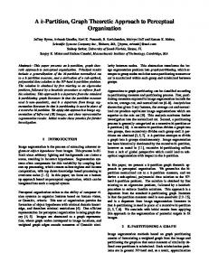
for all i, j iff O(Ai , Bj ) holds for all i, j iff f5 (Ai , Bj ) ≤ (1, 1, 1, 1, 0) for any i, j iff F (A, B) ≤ (1, 1, 1, 1, 0). (7) Note that F5∗ (A, B) = (0, 0, 0, 0, 1) iff DR(Ai , Bi ) holds for all i iff Ai ∩Bi = ∅ iff S(A) ∩ S(B) = An ∩ Bn = ∅ iff Ai ∩ Bj = ∅ for all i, j iff DR(Ai , Bj ) holds for any i, j iff F5 (A, B) = (0, 0, 0, 0, 1). We now give some examples of classifications of topological relations between fuzzy regions with at most two non-zero values, that is, R(V ) for V = {1, α} with 0 < α < 1. Example 4.1 (F ∗ (RCC5) relations) There are 21 F5∗ -modes on R(V ) if α 6= 0.5, and these configurations are illustrated in Figure 1. If α = 0.5, then there are 15 modes on R(V ). Note that any two modes in the following pairs, (2,6), (3,7), (4,8), (10,13), (11,14), (16,18) cannot be distinguished in this case. 2 Example 4.2 (F (RCC5) relations) Write β = 1−α. There are 45 F -modes between fuzzy regions in R(V ) if α 6= 0.5: 1 3 5 7 9 11 13 15 17 19 21 23 25 27 29 31 33 35 37 39 41 43 45

= = = = = = = = = = = = = = = = = = = = = = =

(0, 0, 0, 0, 1), (0, 0, 0, α, β), (0, αβ, 0, α2 , β), (0, αβ + α2 , 0, 0, β), (0, 0, αβ, α, β 2 ), (0, 0, α, αβ, β 2 ), (0, 0, 0, 1, 0), (0, αβ, 0, αβ + α2 + β 2 , 0), (0, β, 0, α, 0), (0, αβ, αβ, α2 + β 2 , 0), (0, α, 0, β, 0), (0, 1, 0, 0, 0), (0, αβ + α2 + β 2 , 0, αβ, 0), (0, αβ, α, 0, β 2 ), (αβ, 0, α2 + β, 0, 0), (0, β, αβ, α2 , 0), (0, α, αβ, 0, β 2 ), (0, α, β, 0, 0), (0, α2 + β, αβ, 0, 0), (β 2 , αβ, α, 0, 0), (α2 , αβ, αβ, 0, β 2 ), (α2 , αβ, β, 0, 0), (α2 + β 2 , αβ, αβ, 0, 0).

2 4 6 8 10 12 14 16 18 20 22 24 26 28 30 32 34 36 38 40 42 44

= = = = = = = = = = = = = = = = = = = = = =

(0, 0, 0, α2 , β + αβ), (0, 0, αβ, α2 , β), (0, 0, αβ + α2 , 0, β), (0, 0, 0, 2αβ + α2 , β 2 ), (0, αβ, 0, α, β 2 ), (0, α, 0, αβ, β 2 ), (0, 0, αβ, αβ + α2 + β 2 , 0), (0, 0, β, α, 0, 0), (0, αβ, αβ, α2 , β 2 ), (0, 0, α, β, 0), (0, 0, 1, 0, 0), (0, 0, αβ + α2 + β 2 , αβ, 0), (0, αβ, β, α2 , 0), (0, αβ, α, β 2 , 0), (0, αβ, α2 + αβ + β 2 , 0, 0), (0, β, α, 0, 0), (0, α, αβ, β 2 , 0), (αβ, α + β 2 , 0, 0, 0), (β 2 , αβ, αβ, α2 , 0), (β 2 , αβ + α2 , αβ, 0, 0), (α2 , αβ, αβ, β 2 , 0), (α2 , β, αβ, 0, 0),

The latter classification of fuzzy regions differs from the one given in [9] through the egg-yolk calculus only in that our mode 3 is divided into Case 3 and Case 4 there. Suppose A = (A1 , A2 ) and B = (B1 , B2 ) are two “egg-yolk” regions, then (A, B) is in Case 3 iff DR(A1 , B1 ), DR(A1 , B2 ), PO(A2 , B1 ), PO(A2 , B2 ); and (A, B) is in Case 4 iff DR(A1 , B1 ), PO(A1 , B2 ), DR(A2 , B1 ), PO(A2 , B2 ). But by Eq.(3), we have F5 (A, B) = (0, 0, 0, α, β) in both situations. 11

1=(1,0,0,0,0)

8=(β,0,0,α,0)

15=(0,0,1,0,0)

9=(0,1,0,0,0)

16=(0,0,α,β,0)

3=(α,0,β,0,0)

10=(0,α,β,0,0)

17=(0,0,α,0,β)

4=(α,0,0,β,0)

11=(0,α,0,β,0)

18=(0,0,β,α,0)

2=(α,β,0,0,0)

... 5=(α,0,0,0,β) .... 12=(0,α,0,0,β) ... ... ... ... ... ... 6=(β,α,0,0,0) .... 13=(0,β,α,0,0) ... ... ... ... ... ... 7=(β,0,α,0,0) .... 14=(0,β,0,α,0) ... ... ... ... ... ...

19=(0,0,0,1,0)

20=(0,0,0,α,β)

21=(0,0,0,0,1)

Figure 1: Illustration of 21 JEPD topological relations between fuzzy regions. The framed, solid line box(es) represents fuzzy region A and the dashed line box(es) represents fuzzy region B, and β = 1 − α.

12

If α = 0.5, there are 37 modes for R(V ). 2 In [9], the authors classify the spatial relations between “egg-yolk” regions using the RCC5 theory. The following example provides a classification of topological relations between vague regions based on the RCC8 theory. Example 4.3. (F ∗ (RCC8) relations) If we use Equation (4) to define approximate spatial relations, we will obtain 51 modes (F ∗ -mode) for R(V ) if α 6= 0.5. If α = 0.5, there are 40 modes for R(V ). We omit details here. 2 In above examples we only consider the special case where the value set V contains exactly two non-zero elements, the method proposed in this paper will be a very powerful tool for classifying topological relations between fuzzy regions with a larger value set. Moreover, based on this classification method and fuzzy set theory, there are also reasonable compositional reasoning methods for spatial reasoning. We shall present these in the following section.

5

Spatial reasoning based on relational composition

In this section we shall propose two relational composition operators based on fuzzy set theory and the RCC l composition table for the F (RCC l) and F ∗ (RCC l) relations defined in Section 4. We also investigate some relation-algebraic aspects concerning these two operators.

5.1

Two relational composition operators

As in above sections, we assume V = {α1 , · · · , αn } and 1 = α1 > α2 > · · · > αn > 0 = αn+1 . Recall F (RCC l) and F ∗ (RCC l) are JEPD sets of topological relations between V -valued fuzzy regions. Note also that we make no distinction between a mode m in Ml or in M∗l and its corresponding relation Rm in F (RCC l) x2 x1 or F ∗ (RCC l). Moreover a mode m = (x1 , · · · , xl ) can be written as EQ + PP + x3 x4 x5 x1 x2 x3 x4 x5 x6 x7 x8 + + or + + + + + + + according to PP∼ PO DR EQ TPP TPP∼ NTPP NTPP∼ PO EC DC l = 5 or l = 8. We also make the following assumption: for l = 5, we write in order EQ, PP, PP∼ , PO, DR as R1 , · · · , R5 and, for l = 8, we write in order EQ, TPP, TPP∼ , NTPP, NTPP∼ , PO, EC, DC as R1 , · · · , R8 . Furthermore, for two RCC l base relations Ri and Rj , we write Rij the composition of Ri and Rj in the RCC l composition table, hence Rij is disjunction of some base RCC l relations. In what follows, when some modes m1 , · · · , mk (k ≥ 2) are addressed together, we assume these modes are altogether in either F (RCC l) or F ∗ (RCC l) for l = 5 or l = 8. Now, for two modes m1 = (x1 , · · · , xl ) and m2 = (y1 , · · · , yl ), we can define their composition by determining the k-th (1 ≤ k ≤ l) coordinate of their composition. We now define m1 ◦w m2 , the weak composition of m1 and m2 , and m1 ◦s m2 , the strong composition of m1 and m2 as follows: k

(m1 ◦w m2 ) =

l M l M i=1 j=1

13

(xi ∧ yj )Rkij .

(5)

k

(m1 ◦s m2 ) = L

l _ l _

(xi ∧ yj )Rkij .

(6)

i=1 j=1

L P Where the operation in (5) is the bounded sum defined as ni=1 xi = ( ni=1 xi )∧1 and (m1 ◦w m2 )k , (m1 ◦s m2 )k and Rkij are, respectively, the k-th coordinate of vectors m1 ◦w m2 , m1 ◦s m2 and Rij . Clearly both operators are partial functions from [0, 1]l × [0, 1]l to [0, 1]l . Recall two vectors v, v 0 in [0, 1]l are related by v ≤ v 0 if vi ≤ vi0 for each i, where vi is the i-th coordinate of v. We have the following Proposition 5.1. Let m1 = (x1 , · · · , xl ) and m2 = (y1 , · · · , yl ) be two modes. Then m1 ◦s m2 ≤ m1 ◦w m2 . W L Proof. It follows from the inequality ni=1 xi ≤ ni=1 xi . Theorem 5.1. Let m1 = (x1 , · · · , xl )P and m2 = (y1 , · · · , yl ) be two modes and suppose m1 ◦w m2 = (z1 , · · · , zl ). Then ni=1 zi ≥ 1. P Proof. If there exists some k with zk ≥ 1, then li=1 zi ≥ 1 clearly holds. So we L l Ll suppose zk < 1 for any k = 1, · · · , l. Then by definition, zk = j=1 (xi ∧ i=1 P P l l yj )Rkij = i=1 j=1 (xi ∧ yj )Rkij , where Rkij ∈ {0, 1} is the k-th coordinate of the P vector Rij . Write Tk = {(i, j) : 1 ≤ i, j ≤ l, Rkij = 1}. Then zk = 1 ∧ {xi ∧ yj : (i, j) ∈ Tk }. For any i, j with 1 ≤ i, j ≤ l, since Rij is a non-empty join of some base RCC l relations, we have some k with Rkij = 1 and hence (i, j) ∈ Tk . This P P P S shows lk=1 Tk = {1, · · · , l} × {1, · · · , l}. Therefore lk=1 zk = lk=1 (1 ∧ {xi ∧ yj : P P P S (i, j) ∈ Tk }) ≥ 1 ∧ {xi ∧ yj : (i, j) ∈ lk=1 Tk } = 1 ∧ li=1 lj=1 xi ∧ yj ≥ P P 1 ∧ li=1 lj=1 xi yj = 1. The latter equation is because that m1 , m2 are two modes Pl P and li=1 xi = 1, i=1 yi = 1. Remark 5.1 Let m1 , m2 be two modes. Denote by D(m1 , m2 ) the set of all possible modes m3 which satisfies the following condition: (∃A, B, C ∈ R(V ))(Am1 B & Bm2 C & Am3 C). (7) W Then it is necessary to require that m1 ◦ m2 = D(m1 , m2 ) for the composition inference ◦ of m1 and m2 . In general, for two modes m1 and m2 , m1 ◦s m2 and m1 ◦w m2 could not be represented by joins of some basic models sometimes(see examples below). This phenomenon is not perfect for the reasoning of spatial relations. To amend this lack, we could use those basic modes which are closed to m1 ◦s m2 or m1 ◦w w2 as the composition inference of m1 and m2 . Then we formalize the following definition of approximate composition reasoning of fuzzy spatial relations. Definition 5.1 For two modes m1 , m2 , let Dw (m1 , m2 ) = {m : m ≤ m1 ◦w m2 }, and Ds (m1 , m2 ) = {m : m ≤ m1 ◦s m2 }. We call Dw (m1 , m2 ) the weak composition inference, Ds (m1 , m2 ) the strong composition inference, of m1 and m2 , respectively. Of course, if the fuzzy spatial relations m1 and m2 are crisp, then the approximate composition inference is just the classical ones (i.e., composition tables). 14

P Remark 5.2 Note that if m1 ◦s m2 = (z1 , · · · , zl ), li=1 zi is not necessary greater than 1, the strong composition inference of m1 and m2 may be empty. On the other hand, by Proposition 5.1 and Theorem 5.1, if m1 ◦w m2 = (z1 , · · · , zl ), we have Pl z i=1 i ≥ 1 and m1 ◦s m2 ≤ m1 ◦w m2 . It is reasonable that there is mode m such that m ≤ m1 ◦w m2 . The composition inference corresponding to weak composition is therefore not empty. On the other hand, because of Definition 5.1, we can define other two fuzzy composition operations on fuzzy spatial relations corresponding to weakly and strong composition inferences. That is, for two models m1 and m2 , _ m1 ◦1 m2 = {m : m ∈ Dw (m1 , m2 )} m 1 ◦2 m 2 =

_

{m : m ∈ Ds (m1 , m2 )}

In general, m1 ◦1 m2 6= m1 ◦w m2 and m1 ◦2 m2 6= m1 ◦s m2 . Since m1 ◦1 m2 is determined by Dw (m1 , m2 ) and m1 ◦2 m2 is determined by Ds (m1 , m2 ), we only discuss the composition inference Dw and Ds in the following. In the following two examples we choose the JEPD set F ∗ (RCC5) given in Example 4.1 as our base of compositions. Example 5.1 Choose F ∗ (RCC5) given in Example 4.1 and assume α < β. We give some weak compositions of F (RCC5) using Equation (5). For any m ∈ F (RCC5), 1 ◦w m = m ◦w 1 = m, i.e. 1 is the identity of the composition operation ◦w . 2 ◦w 2 = (α, 1, 0, 0, 0) = 2 ∨ 9. Dw (2, 2) = {2, 9}. 2 ◦w 3 = (1, 1, 1, β, β) = 1 ∨ 2 ∨ 3 ∨ 4 ∨ 5 ∨ 6 ∨ 7 ∨ 8 ∨ 9 ∨ 10 ∨ 11 ∨ 12 ∨ 13 ∨ 14 ∨ 15 ∨ 16 ∨ 17 ∨ 18 ∨ 20. Dw (2, 3) = {1, 2, 3, 4, 5, 6, 7, 8, 9, 10, 11, 12, 13, 14, 15, 16, 17, 18, 20}. 2 ◦w 4 = (α, 1, 0, 1, β) = 2 ∨ 4 ∨ 5 ∨ 9 ∨ 11 ∨ 12 ∨ 14 ∨ 19 ∨ 20. Dw (2, 4) = {2, 4, 5, 9, 11, 12, 14, 19, 20}. 2 ◦w 5 = (α, α, 0, 0, 1) = 5 ∨ 12 ∨ 21. Dw (2, 2) = {5, 12, 21}. 2 ◦w 21 = (0, 0, 0, 0, 1) = 21. Dw (2, 21) = {21}. 5 ◦w 6 = (α, 2α, 0, α, 1) can not be represented as finite disjunction of modes. Dw (5, 6) = 5 ∨ 12 ∨ 20 ∨ 21 if 2α < β, and Dw (5, 6) = 5 ∨ 2 ∨ 12 ∨ 14 ∨ 20 ∨ 21 if 2α ≥ β. 2 ∗ Example 5.2 Choose F (RCC5) given in Example 4.1 and assume α < β. We give some strong compositions of F (RCC5) using Equation (6). For any m ∈ F (RCC5), 1 ◦s m = m ◦s 1 = m, i.e. 1 is the identity of the composition operation ◦s . 2 ◦s 2 = 2. Ds (2, 2) = {2}. 2◦s 3 = (β, β, β, β, β) = 2∨3∨4∨5∨6∨7∨8∨10∨11∨12∨13∨14∨16∨17∨18∨20. Ds (2, 3) = {2, 3, 4, 5, 6, 7, 8, 10, 11, 12, 13, 14, 16, 17, 18, 20}. 2 ◦s 4 = (α, β, 0, β, β) = 2 ∨ 4 ∨ 5 ∨ ∨11 ∨ 12 ∨ 14 ∨ 20. Ds (2, 4) = {2, 4, 5, 11, 12, 14, 20}. 15

2 ◦s 5 = (α, α, 0, 0, β) = 5 ∨ 12. Ds (2, 5) = {5, 12}. 2 ◦s 21 = (0, 0, 0, 0, β), there is no mode contained in 2 ◦s 21, since the sum of components of 2 ◦s 21 is less than 1. Ds (2, 21) = ∅. 5 ◦s 6 = (α, α, 0, α, β) = 5 ∨ 12 ∨ 20. Ds (5, 6) = {5, 12, 20}. 2

5.2

Relation-algebraic aspects of approximate spatial reasoning

Set V = {α1 , · · · , αn } and 1 = α1 > α2 > · · · > αn > 0 = αn+1 . Recall F (RCC l) and F ∗ (RCC l) are JEPD sets of topological relations on R(V ), the collection of V -valued fuzzy regions. Based on the two composition operations defined in Section 5.1, we can consider some relation-algebraic aspects of spatial reasoning involving fuzzy regions as done in [14, 27] for crisp regions. We summarize some basic results for these operations. Theorem 5.2. Suppose m1 , m2 , m3 are three modes, then the following statements hold, where the operator ◦ can be either the weak composition ◦w or the strong composition ◦s . (1) (m1 ◦ m2 ) ◦ m3 = m1 ◦ (m2 ◦ m3 ); (2) (m1 ◦ m2 )∼ = m2 ∼ ◦ m1 ∼ ; (3) (m1 ∼ )∼ = m1 . (4) There exists a mode m which is the identity relation on R(V ). Proof. We consider only the case where the modes are taken from F (RCC5) and the operator is the strong composition ◦s , the other cases are similar. Suppose m1 , m2 , m3 ∈ F (RCC5), and let m1 = (x1 , x2 , x3 , x4 , x5 ), m2 = (y1 , y2 , y3 , y4 , y5 ), m3 = (z1 , z2 , z3 , z4 , z5 ). (1) Note that W W (m1 ◦s m2 ) ◦s m3 = ( i j (xi ∧ yj )(Ri ◦s Rj )) ◦s m3 W W W (x ∧ yj ∧ zk )((Ri ◦s Rj ) ◦s Rk ) = Wi Wj Wk i = i j k (xi ∧ yj ∧ zk )(Ri ◦s (Rj ◦s Rk )) = m1 ◦s (m2 ◦s m3 ) W W W ∼ ∼ ∼ (2) Since m ◦ m = (x ∧ y )(R ◦ R ) and m = = 1 s 2 i j i s j 1 i j i x i Ri , m 2 W ∼ y R , we have i i i W W (m1 ◦s m2 )∼ = (x ∧ yj )(Ri ◦s Rj )∼ Wi Wj i ∼ ∼ = i j (xi ∧ yj )(Ri ◦s Rj ) = m2 ∼ ◦s m1 ∼ . (3) Clear by definition. (4) Note that (1, 0, 0, 0, 0) ◦s m1 = m1 ◦ (1, 0, 0, 0, 0) = m1 holds for any m1 .

16

6

Conclusions and future work

This paper is mainly concerned with the representation and reasoning aspects of topological relations between fuzzy regions. We give a general approach for classifying topological relations between fuzzy regions based on the RCC theory and fuzzy set theory. We also introduce two operators of relational composition for these topological relations. Some aspects of relation-algebraic properties of these composition operators are also investigated. Note that neither modelling crisp region as non-empty regular closed set nor the choice of RCC5 and RCC8 relations are compulsory. The approach proposed in this paper can be generalized in two orthogonal directions: on one hand, we can restrict our domain of crisp regions to be either the set of closed disks or the set of simple regions in the sense of, e.g. [6], or some other domain which support the RCC5 and RCC8 CT (see [26]); on the other hand, this approach is applicable to other formal theories of binary relations, for example the 13 interval relations given in [1] or the RCC11 theory developed in [13]. In particular, our methods for defining binary topological relations between V valued fuzzy regions are applicable to both (general complex ) fuzzy regions (as the previous sections of this paper have shown) and simple fuzzy regions without holes in the sense of, e.g., Zhan [39]. Note that the domain of corresponding crisp regions of simple fuzzy regions is the collection of simple regions, namely the set of connected closed sets bounded by a closed Jordan curve. Since this domain of crisp regions also supports the RCC8 CT [17, 26] (hence also supports the RCC5 CT), our methods can also be applied to simple fuzzy regions with a little modification. There are still many important issues about spatial reasoning involving fuzzy regions that should be further researched, e.g. the choice of a reasonable approach for compositional inference, the relation between composition inference introduced in this paper and the CRI (Compositional Rule of Inference) approach introduced by Zadeh [38], the complexity ([32]) of spatial reasoning involving fuzzy regions, and the most important, the application of the approach to GIS and AI. Acknowledgements: This work was done during the first author visiting Tsinghua University. He would like to express thanks to Professor Mingsheng Ying for his invitation and his great help. The authors are grateful to the anonymous referees who suggested several improvements and pointed out a missing reference in the previous version of this paper.

References [1] J.F. Allen, Maintaining knowledge about temporal intervals, Communications of the ACM 26(1983)832-843. [2] D. Altman, Fuzzy set theoretic approaches for handling imprecision in spatial analysis, International Journal of Geographical Information Systems 8(1994)271-289. [3] T. Bittner, J.G. Stell, Approximate spatial reasoning, Spatial Cognition & Computation 2(2000)435-66. 17

[4] I. Bloch, Fuzzy relative position between objects in image processing: a morphological approach, IEEE Trans. Pattern Analysis and Machine Intelligence 21(1999)7:657-664. [5] P.A. Burrough, A.U. Frank, Geographic Objects with Indeterminate Boundaries, Taylor & Francis, London, 1996. [6] E. Clementini, P. Di Felice, Approximate topological relations, Int.J. Approximate Reasoning 16(1997)173-204. [7] A.G. Cohn, The Challenge of Qualitative Spatial Reasoning, Computing Surveys27(1995)323-326. [8] A.G. Cohn, B. Bennett et al., Qualitative Spatial Representation and Reasoning with the Region Connection Calculus, GeoInformatica 1(1997)275-316. [9] A.G. Cohn, N.M. Gotts, The ‘egg-yolk’ representation of regions with indeterminate boundaries, in: [5], pp. 171-187, 1996. [10] H. Couclelis, A typology of geographic entities with ill-defined boundaries, in: [5], pp. 45-55, 1996. [11] Z. Cui, A.G. Cohn, D.A. Randell, Qualitative and topological relationships in spatial databases, in D. Abel and B. C. Ooi (Eds.), Advances in Spatial Databases, Lecture Notes in Computer Science 692, Springer Verlag, Berlin, pp. 293-315, 1993. [12] S. Dutta, Qualitative spatial reasoning: a semi-quantitative approach using fuzzy logic, in A. Buchman, O. G¨ unther, T.R. Smith, Y.F. Wang (Eds.)Design and implementation of large spatial information databases, Lecture Notes in Computer Science 409, Springer-Verlag, Berlin, pp. 345-364, 1989. [13] I. D¨ untsch, A tutorial on relation algebras and their application in spatial reasoning, Given at COSIT, August 1999. [14] I. D¨ untsch, H. Wang, S. McCloskey, A relation-algebraic approach to the region connection calculus, Theoretical Computer Science 255(2001)63-83. [15] D. Dubois, M.C. Jaulent, A general approach to parameter evaluation in fuzzy digital picture, Pattern Recognition Letters 6(1987)251-259. [16] D. Dubois, H. Prade, On several representations of an uncertain body of evidence, in: M.M. Gupta and E. Sanchez (Eds.), Fuzzy Information and Decision Processes. North-Holland, Amsterdam, pp.167-181, 1982. [17] M.J. Egenhofer, Reasoning about binary topological relations, in: O. G¨ unther, H.-J. Schek (Eds.), Advances in Spatial Databases, Lecture Notes in Computer Science 525, Springer, New York, pp.143-160, 1991. [18] M.J. Egenhofer, R. Franzosa, Point-set topological spatial relations, International Journal of Geographical Information Systems 5(1991)161-174. 18

[19] C. Freksa, Temporal reasoning based on semi-intervals, Artificial Intelligence 54(1992)199-217. [20] H. Guesgen, Fuzzifying spatial relations, in: P. Matsakis, L.M. Sztandera (Eds.) Applying Soft Computing in Defining Spatial Relations, Physica-Verlag, Berlin, pp.1-15, 2002. [21] J.L. Kelley, General Topology, Van Nostrand, New York, 1955. [22] L. Kulik, A geometric theory of vague boundaries based on supervaluation, in: D.R. Montello(Ed.) Spatial information sciences:fundations of Geographic Information Science, Lecture Notes in Computer Science 2205, Springer, Berlin, pp.44-59, 2001. [23] R. Krishnapuram, J.M. Keller, Y. Ma, Quantitative analysis of properties and spatial relations of fuzzy image regions, IEEE Trans. Fuzzy Syst.1(1993)3:222233. [24] Y. Leung, On the Analysis19(1987)125-151.

imprecision

of

boundaries,

Geographical

[25] S. Li, M. Ying, Region Connection Calculus: Its models and composition table, Artificial Intelligence145(2003)121-146. [26] S. Li, M. Ying, Extensionality of the RCC8 composition table, Fundamenta Informaticae55(3-4)(2003)363-385. [27] Y. Li, S. Li, M. Ying, Extensionality and representation of RCC11 composition table, (submitted for publication). [28] Z. Pawlak, Rough Sets: Theoretical Aspects of Reasoning about Data, Kluwer, Dordrecht, 1992. [29] D.A. Randell, A.G. Cohn, Z. Cui, Computing transitivity tables: A challenge for automated theorem provers, Proceedings CADE 11, Springer Verlag, Berlin, 1992. [30] D.A. Randell, Z. Cui, A.G. Cohn, A spatial logic based on regions and connection. in: B. Nebel, W. Swartout, C. Rich (Eds.), Proceedings of the 3rd International Conf Knowledge Representation and Reasoning, Morgan Kaufmann, Los Allos, CA, pp.165-176, 1992. [31] J. Renz, Qualitative spatial reasoning with topological information, Lecture Notes in Artificial Intelligence 2293, Springer-Verlag, Berlin, Germany, 2002. [32] J. Renz, B. Nebel, On the complexity of qualitative spatial reasoning: A maximal tractable fragment of the Region Connection Calculus, Artificial Intelligence 108(1999)69-123. [33] A. Rosenfeld, Fuzzy digital topology, Information and control 40(1979)76-87.

19

[34] A.J. Roy, J.G. Stell, Spatial relations between indeterminate regions, Int. J. Approximate Reasoning 27(2001)205-234. [35] M. Schneider, Uncertainty management for spatial data in databases: fuzzy spatial data types, in: R.H. G¨ uting, D. Papadias, F. Lochovsky (Eds.) Advances in Spatial Databases Lecture Notes in Computer Science 1651, Springer-Verlag, Berlin, Germany, pp.330-51, 1999. [36] F. Wang, G.B. Hall, Fuzzy representation of geographical boundaries in GIS, International Journal of Geographical Information Systems 10(1996)573-590. [37] M. Worboys, Imprecision in finite resolution spatial data, GeoInfomatica 2(1998)257-279. [38] L.A. Zadeh, Fuzzy sets, Information and Control 8(1965)338-353. [39] F.B. Zhan, Approximate analysis of binary topological relations between geographical regions with indeterminate boundaries, Soft Computing 2 (1998)2834. [40] H.J. Zimmermann, Fuzzy Sets Theory and its Applications, Boston: Kluwer Academic Publisher, 1991.

20