A Gaussian Weave for Kinematical Loop Quantum Gravity

A Gaussian Weave for Kinematical Loop Quantum Gravity A. Corichi1∗ and J. M. Reyes1,2† 1 Instituto

arXiv:gr-qc/0006067v2 3 Aug 2000

de Ciencias Nucleares, Universidad Nacional Aut´ onoma de M´exico A. Postal 70-543, M´exico D.F. 04510, M´exico. 2 Departamento de F´ ısica, Centro de Investigaci´ on y de Estudios Avanzados del IPN A. Postal 14-740, M´exico D.F. 07000, M´exico. (February 7, 2008)

Abstract Remarkable efforts in the study of the semi-classical regime of kinematical loop quantum gravity are currently underway. In this note, we construct a “quasi-coherent” weave state using Gaussian factors. In a similar fashion to some other proposals, this state is peaked in both the connection and the spin network basis. However, the state constructed here has the novel feature that, in the spin network basis, the main contribution for this state is given by the fundamental representation, independently of the value of the parameter that regulates the Gaussian width.

Typeset using REVTEX

∗ Electronic

address: [email protected]

† Electronic

address: [email protected]

1

I. INTRODUCTION

One of the most important physical results of loop quantum gravity [1] is the prediction that the spectra of geometric operators, corresponding to their classical analogues such as areas of surfaces and volumes of regions, are purely discrete [2,3]. Some other intriguing features of this ‘Non-perturbative Quantum Geometry’ have emerged already at the kinematical level, for example, the non-commutativity of geometric operators [4], and the statistical derivation of Black Hole entropy [5]. Despite the relative success of the canonical/loop quantum gravity approach, two major problems need to be successfully tackled: dynamics (that is, a complete and anomaly-free implementation of the quantum Hamiltonian constraint) and the recovery of general relativity as a low energy/macroscopic regime of the quantum theory. How could the two problems be related is an open question, but it is likely that a complete understanding of the quasi-classical regime of the theory at the kinematical level (in particular states which can approximate functions of connections) can give some insight into the dynamics of the theory [6]. In this approach, General Relativity (GR) has to arise from the semi-classical limit of the quantum theory through properly defined ‘coherent states’ and a suitable coarse-graining. Coherent states have been constructed only recently in loop quantum gravity [7]. However, we shall argue that some important issues have to be addressed first in order to obtain a complete understanding of the problem. At the kinematical level, the first attempts in this direction were given by the so called ‘weave states’ in the old loop representation [8]. As originally constructed, weave states were intended to be semi-classical states (initially, eigenstates of geometrical operators) that approximate smooth geometries on a background spatial (and compact) 3-manifold Σ for large scales. That is, given a fiducial metric on Σ, the spatial average of expectation values of area and volume operators in this state should be given by their classical values as measured by the fiducial 3-metric on Σ above some macroscopic scale L. There is increasing hope that once one has a good candidate for a weave describing flat space, one would be able to develop quantum field theory (QFT) on these states. There are some evidences pointing out in the direction that QFT’s on weaves would be free of infinities and should not require any renormalization procedure [9]. Another important issue that deserves further attention is whether semi-classical states can be promoted to solutions to the Hamiltonian constraint of the theory. It is well known that eigenstates of 3-geometries are not suitable states describing 4-dimensional Minkowski space-time, as happens, for instance, in quantum electrodynamics (QED) where an eigenstate of the electric field operator with null eigenvalue has a very different physical meaning than that of QED vacuum [10]. However, kinematical results could be important by themselves in situations where classical boundary conditions such as asymptotical flat space times [11] and isolated black holes boundary conditions are imposed on the system [6,5]. Recent attempts in constructing weaves were given in [12] with the use of ‘spin networks’, and have been recently used as a background ‘thermal’ state to construct new Hilbert spaces for non-compact spaces [11]. Nevertheless, weaves are defined based on the behavior of geometrical operators that depend only in momentum variables and therefore, only provide information about half of the classical phase space while the behavior of some connection variable operators might not be under control in these states. In fact, the original weaves were expected to be ‘concentrated’ in geometry, so they are highly delocalized in the con2

nection variable and the fluctuations of the configuration operators might be very large. For instance, it has been recently shown that the natural strategy for approximating connections by taking the elementary configuration variable, namely the SU(2) holonomy, as the multiplicative operator, fails [6]. Any attempt to reproduce their classical analogue is doomed since there are no quantum states that support such supposition and such that they satisfy additional minimum uncertainty relations [6]. Instead, a more ambitious proposal has been given by the authors of [6] and consists on a tentative definition of ‘quasi-classicity’, a latticization of the underlying manifold and the use of ‘magnetic flux’ type operators. This was the first step in attempting to construct within the loop approach, realistic semi-classical states at the kinematical level (in the simplified case of two spatial dimensions). More recently, a series of papers by Thiemann and Winkler have appeared in which semi-classical states are constructed from a (complex) coherent-state transform on phase space (see [7] and references therein). In this work we follow the same strategy as in [11], namely we construct an (invertible) weave state based on a cylindrical function, that might serve as background for the construction of new Hilbert spaces when the space is non-compact. There is however, an important difference between our weave state and the one originally proposed in [11]: Our state depends in a ‘Gaussian way’, i.e. on a suitable exponential arrangement of square of group elements. The state constructed here is peaked around the trivial ‘flat’ connection that yields the identity element for the holonomy around each loop defining the state. With this prescription, one might hope to overcome the objection previously raised regarding large fluctuations for (every) holonomy operator. In this sense, if one is able to reproduce the flat (metric) behavior through the geometric operators, and the connection is also ‘peaked’ around the flat connection, one might hope to have a semi-classical state approximating Minkowski space-time. It is worth mentioning that the exponential dependence on group elements is a common feature of coherent states in compact Lie groups [13]. We will show that this one-parameter family of states has better behavior than the original ‘quasi-coherent’ weave, and that in this case, the states are peaked and centered around the fundamental representation, when written in the spin network basis. This result is particularly intriguing, since a similar behavior, i.e., a dominance of the fundamental representation, is also observed in the computation of the black hole entropy [5]. This paper is organized as follows: In Section II we give a very brief review of the most important facts of loop quantum gravity that are relevant for this work. Readers familiar with the loop formalism may want to skip to Section III where the notion of a weave state is recalled. In the Section III B we proceed to the construction of the ‘Gaussian’ weave which approximates flat space. We also take the opportunity to make some general observations and, in particular, we discuss some subtleties that arise when an eigenbasis of the area operator is introduced. We close with a discussion in Section IV. II. PRELIMINARIES

Canonical/Loop quantum gravity is a canonical approach for quantizing general relativity in a non-perturbative way. In this approach, general relativity is a purely constrained system, 3

a feature for all diffeomorphism invariant theories. A rigorous kinematical framework to handle theories whose classical configuration space is given by connections moduli local gauge transformations, has been constructed in the past decade [14]. General relativity can be written in this form using the so-called Ashtekar-Barbero variables [15]. In this section we summarize the main results of this approach. The classical phase space consists of canonical pairs of a SU(2) valued connection Aia on an orientable spatial 3-manifold Σ and its conjugate momentum variable, a densitized triad Eia which takes values in the dual of the Lie algebra [15]. The dynamics of the theory, for compact Σ, is pure gauge and is encoded in the Gauss constraint which generates SU(2) gauge transformations, the spatial 3-dimensional diffeomorphism constraint generating spatial 3d diffeomorphisms on Σ, and the Hamiltonian constraint which generates the coordinate time evolution. The classical configuration space A, is given by the space of all smooth connections on a principal SU(2) bundle over Σ. Since A is infinite dimensional the quantum configuration space A is a certain completion of the classical one which includes all ‘distribution-like’ connection, in a similar role played in free field theory in Minkowskian space by the tempered distributions. Hence A is taken to be the space of generalized connections which have a well defined action on oriented paths over Σ and the group of generalized SU(2) gauge transformations [14]. Since A is compact it admits a regular diffeomorphism-invariant measure dµo and the Hilbert space can be taken to be the space H = L2 (A, dµo) of square-integrable functions on A. This space is actually non-separable, but we can associate quantum states of the gauge theory to finite graphs γ 1 . If we consider all possible graphs, we obtain a very large set of states which are dense on H. These states defined on finite graphs are called cylindrical functions and depend on finite sets of holonomies along the edges of the graph. Therefore, given any complex valued function ψ : (SU(2))n → C we can associate a cylindrical function Ψγ (A) ∈ Aγ as follows: Ψγ,ψ (A) = ψ(he1 (A), .., hen (A)).

(2.1)

hei denote the SU(2) parallel propagator matrices of the connection A ∈ A along the curve ei . Exploiting the compactness of SU(2) the space of cylindrical functions C is equipped with the inner product: Z (2.2) ψ1 (he1 , .., hen )ψ2 (he1 , .., hen )dµH (he1 ) . . . dµH (hen ) hΨγ1 ,ψ1 | Ψγ2 ,ψ2 i = SU (2)n

where dµH (he1 ) . . . dµH (hen ) is the n-copy Haar measure naturally induced from SU(2). If the graphs γ1 and γ2 are different, the respective cylindrical functions can be viewed as being defined in the same graph, which is the union of both: γ1 ∪ γ2 . The classical algebra of elementary observables S consist of the set of canonical variables Aia and eabi := ηabc Eic smeared against suitable fields which in this case are one dimensional

1 For

simplicity we will take the paths to be analytic embedded.

4

for the connection, and two-dimensional for the triad field [4]. The space of configuration variables is given by the space Cyl of functions of the type (2.1), when the graph γ is varied over all arbitrary finite graph. The momentum variables are obtained by smearing the pseudo 2-forms eabi against a test field f i which takes values in the Lie-algebra of SU(2). Z 2 E[S, f ] = eabi f i dS ab . (2.3) S

Here, the surface S is restricted to be of the type S = S − ∂S, where S is any compact, analytic 2-dimensional sub-manifold of Σ possibly with boundary. See [4] for details and [16] for an alternative choice of variables. The standard representation of the quantum algebra on H is to have the cylindrical (configuration) functions act as multiplicative operators, and “electric flux” variables as certain derivative operators [4]. When the spatial slice Σ is non-compact, a quantum state that describes, say, an asymptotically-flat space requires an infinite volume (and a contribution to this volume coming from everywhere within Σ). This in turn, implies that the state must have contributions from graphs with an infinite number of edges. This state would not, in particular, belong to our Hilbert space H. In order to have a formalism that would allow for these situations, Arnsdorf and Gupta have proposed an algebraic construction, a la GNS, to overcome this difficulty. The basic idea is to construct new Hilbert spaces where a particular, semiclassical, non-normalizable state would serve as a vacuum of the theory, and the ordinary normalizable states would be seen as ‘finite excitations’ of the geometry. For details of the construction see [11]. For our purposes, it is enough to know that the formalism requires an invertible state, that is, a state that does not vanish for any point on A, and that has support on an infinite number of edges. In the next section we shall construct such an state. III. APPROXIMATING FLAT SPACE

This section has two parts. In the first one we recall the general definition of a weave state. In the second part, we construct a Gaussian weave and show that it satisfies the requirements for a decent weave state and that it has some interesting features that make it an acceptable candidate for a quantum theory on non-compact spaces. A. General Framework

In any quantum field theory, the semi-classical regime is obtained or represented by two main ingredients: “coherent states” and a suitable coarse graining. However, in the case of the gravitational field additional problems arise since the notion of “vacuum state” is not provided a priori, unless one forces it by splitting the metric into a preferred vacuum metric (usually taken flat) and a perturbative term whose fluctuations define the quantum theory. In the other hand, in canonical/loop quantum gravity, as in any other non-perturbative approach to quantum gravity, the natural ‘vacuum state’ corresponds to the ‘no metric’ space gab = 0. In this case flat space becomes a highly excited state of the 3-geometry, containing an infinite number of fundamental excitations. Weave states are kinematic states constructed 5

to provide semi-classical metric information over the spatial 3-manifold Σ, that is, they approximate flat space above some macroscopic scale L. However, since the spatial metric gab is constructed completely from momentum variables (densitized triads), weaves are normally thought to be highly concentrated in geometry, and it is possible that certain configuration variables, when promoted to operators, would be wildly delocalized in these states. This would render the weave states as unsuitable candidates for quasi-classical states. However, the weave state that we shall construct here is peaked, in the connection representation, around the flat connection for each loop of the defining graph. Thus, one expects that certain configuration observables be localized on these states. It is important to recall that all relevant results in the semi-classical regime of the theory have emerged at the kinematical2 level since a complete and anomaly-free implementation of the constraints have not been found successfully. The discrete nature of quantum geometry [2–4,17] provides a suitable criterion for approximating flat space. There are geometric operators which are self-adjoint in the Hilbert space H and that measure areas of surfaces and volumes of regions. Therefore, a classical spatial metric can be approximated by requiring that the expectation values of areas and volumes of macroscopic surfaces and regions correspond to their classical analogues. Let suppose that we want to approximate the Euclidean 3-space R3 with the weave state Φw . The strategy is as follows: Let consider a macroscopic region in R3 (of size larger than L) with bulk R and surface S. We perform successive measurements of the volume of the region VˆR and the area of the surface AˆS on the state Φw at different positions in Σ. The state Φw is called a ‘weave’ state if it satisfies the following requirements: 1. The spatial average of the expectation values of the area S and volume R agree with their classical values. Z p hAˆS iw = | qab | + O(ǫ2 /L2 ), (3.1a) S

hVˆR iw =

Z p | gab | + O(ǫ3 /L3 ),

(3.1b)

R

where L is the characteristic macroscopic size of the bulk and ǫ is a microscopic scale, which is normally taken to be of the order of the Planck length ℓP , qab is the induced metric on S, the “over-line” indicates spatial average and the expectation values are taken in the state Φw . 2. The state Φw must have small quantum fluctuations in the measurements with regard to the macroscopic scale L. δV ≪ L3 δA ≪ L2

2 wherein

the diffeomorphism and Hamiltonian constraint are ignored.

6

(3.2a) (3.2b)

where δV and δA are the standard deviations of the repeated measurements of the volume and area of the corresponding region. Actually, the conditions (3.2) can be satisfied by an infinitely number of quantum states and do not single out a preferred state. In general, one could identify two distinct steps in the construction of a candidate of a weave state. First, one specifies a graph on Σ where the state is supposed to have support (or a family of graphs in a statistical sum). For instance, one could provide a lattice that ‘covers’ the whole space Σ [6], or a ‘unit’ graph γ that is going to be spread over Σ to cover it. The second step involves the specification of a cylindrical function to be living on the basic units of the construction, be it on plaquetes of the lattice in the first case above, or basic cylindric functions on the graph γ. Some explicit examples of both types have been constructed in the literature, the first ones being simultaneous eigenstates of the volume and area operators ( [12], [8]) and a recent ‘quasicoherent’ state [11] with some nice properties. An example of states based on a lattice is given in [6]. In this note, we construct a particular weave state similar in spirit to the one given in [11]. Actually, one is only proposing a cylinder function (i.e., the second step in the construction outlined above), which could in principle be implemented on different graphs. We choose a graph construction first proposed in [12] (and also considered in [11]) for simplicity, and to be able to compare the properties of our Gaussian ansatz with the other proposals. It should be clear from the discussion that one could take our Gaussian ansatz and implement it in other graph/lattice constructions. Our ansatz has the property that it shares some of the nice properties of earlier proposals, that is: it is an invertible state, is peaked in the connection and the spin-network basis. However, it has the particular feature that the peak in the spin-network basis is centered around the fundamental representation. We shall refer to this state as the ‘Gaussian’ weave because it is constructed as a Gaussian function of cylindrical factors. B. The ‘Gaussian’ Weave

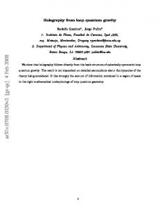
The aim of a weave is to reproduce the area and volume of any region in the slice Σ. Therefore, the graph in which the state is based must fill all Σ and if the space Σ is noncompact, one is left with two options: The graph either consists of edges of infinite length or it is an infinite set of finite graphs. In particular, our weave state is based on a disjoint union of an infinite collection of finite graphs: Gρr = ∪∞ i=1 γi where γi represent the graph of a system of two non-coplanar circles αi and βi with the same radius r respect to a fiducial metric, which intersect in a single vertex, see Fig. 1. These systems of circles are randomly distributed in Σ with average density ρ measured with the same fiducial metric. Let us define the cylindrical function based in the graph γi gi (A) = N exp −(λTr[(he αi (A)he βi (A) − e)(1) ])2 ,

(3.3)

where N is a normalization factor, λ is a positive parameter, he α,β i (A) are the holonomies along the circles α and β respectively and the subindex 1 represents the fundamental representation in SU(2) (Color 1 in the terminology of Penrose). It is worth noting the Gaussian 7

β α

r

v

eβ r

eα FIG. 1. Graph γi as the union of two intersecting circles αi and βi . Note that the intersection is given by a tetravalent vertex.

dependence on group elements. The Gaussian weave can be written as an infinite product of functions (3.3). W = lim

n→∞

n Y

gi (A).

(3.4)

i=1

This state does not belong to the Hilbert space H but is defined through the cylindrical function gi based on the graph γi and can be considered as a candidate for a background (thermal) state for constructing new Hilbert spaces as in [11]. The state (3.4) has common features with that given in [11] and can be considered as a ‘quasi-coherent’ state in the Q same footing. By definition, the cylindrical functions given by the finite product Wn = ni=1 gi (A) take on their maximum values when the holonomies along the circles in the graph γi are the identity in SU(2) and if Ae denote the connection which give the trivial holonomy, as n → ∞ the function Wn become increasingly peaked around Ae . The width of the peak is regulated by the Gaussian parameter λ. We are interested in exploring the main features of the state W and in showing that it satisfies the weave conditions (3.1), and (3.2). For this purpose we begin expanding the cylindrical function gi into the De-Pietri-Rovelli spin-network basis. The only elements of the basis that have a non-vanishing contribution are given by, Φj = Tr[(he αi (A)he βi (A))(j) ],

(3.5)

based on the graph γi, where the subindex j denote the ‘color’ representation of SU(2). This choice arises because Φj can be written as a linear expansion of spin-network states some of which are eigenstates of the area operator for an arbitrary analytic surface S that intersect the graph γi . The fact that these states are not eigenstates of the area operator for any surface is particularly interesting and deserves further explanation. On the full Hilbert space H, and for gauge-invariant cylindrical functions Nγ 3 , the spec-

3 We

will restrict to gauge-invariant states on A. This will be useful because it permits the transition to the loop representation where from the beginning one restrict oneself to gauge invariant states (spin-network states).

8

α

β j

α

β j

j

j

j’

v j

j

j

j

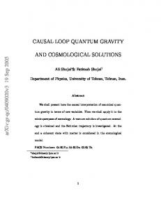
FIG. 2. Decomposition of the tetravalent vertex into two trivalent vertices joined by an ’internal’ edge of color j ′ inside the virtual ribbon-net.

trum of the area operator Aˆ is unbounded from above and the ‘area gap’, which is the smallest non-zero eigenvalue, is given in the special situation when the graph intersect the surface S with an -up or down- edge and a tangential edge at a bivalent vertex v [3]. If a single edge intersect the surface (without crossing S), or if the edges that meets at the vertex v are all ‘up’ or ‘down’, the Gauss law constraint implies that the corresponding eigenvalue be 0. Therefore, to obtain non-trivial eigenvalues of the area operator is necessary that the edges of the graph ‘cross’ the surface S. This means that for the system of circles γi, the state (3.5) is an eigenstate of the area operator with non-trivial eigenvalues if at least one of the circles crosses S, that is, if the same circle intersect the surface in two points (vertices). If one or both of the circles only ‘touch’ the surface in one point, the arcs that meet that point will be at the same side of S and the corresponding eigenvalue would be 0 as was stated above. The maximum number of intersections between γi and the surface is 4 and is obtained when both circles cross S. On the other hand, given the spin-network s = (γi, ~j, ~l) which assigns the labelling ~j = (j, j) to the circles αi and βi of the graph γi with the j representation of SU(2), and a labelling ~l = (l1 ) of the single tetravalent vertex of γi with an invariant tensor c1 , that is, an intertwining tensor from the representations of the incoming edges to the representations of the outgoing edges. The spin-network states can be constructed by contracting the matrices associated to the j representation of the circles on γi with the intertwining tensor c1 at the tetravalent vertex. The basis element (3.5) when written in the spin-network (state) expansion, correspond to the choice of a particular basis of the space of the invariant tensor of the tetravalent vertex, and is given by the Fig. 2 in the De Pietri-Rovelli notation [17]. Graphically, the choice of the basis in the space of invariant tensors is equivalent to the ‘decomposition’ of the tetravalent vertex into a trivalent graph with two vertices joined by a ‘virtual’ edge j ′ . Since the Clebsh-Gordan condition must hold in each of the trivalent vertices, the only allowed value for the virtual vertex is j ′ = 0. Thus, we would be lead to the conclusion that the basis element (3.5) is an eigenstate of the area operator. This is true in general, but it remains the subtle case when the tetravalent vertex of the graph γi lies on the surface S. There are two possible (non-generic) configurations in this special case: 1. The first configuration is obtained when the surface S divides the graph γi into two halfs. Each of them has a part of the circle αi and a part of the circle βi . In this situation, (3.5) has no contribution to the area coming from the vertex (since j ′ = 0) and is then an eigenstate of the area operator with eigenvalues proportional to

9

8πℓ2P

q

j j ( 2 2

+ 1) for each intersection of the circles with S.

2. The other ‘non-generic’ configuration is realized when the surface S divides the graph γi in such way that one of the circles, say αi , is entirely placed on one side of the surface and the circle βi on the other. In this case the basis (3.5) is not an eigenstate of the area operator and it is indispensable the use of the recoupling theorem [17,19] in order to perform the suitable change of basis in which the area operator can take a diagonal form. Even when the state is written in a diagonal form, there will be in general contributions from eigenstates with different eigenvalues for the area. At first sight this seems to be a problem when expanding the Gaussian function (3.3) into the basis elements (3.5) but a closer look shows that the number of ‘pathological’ configurations represents a zero measure set in the collection of all possible configurations. However, even though the configurations with the tetravalent vertex on S do not contribute in a significant way to the expansion of the function (3.3), they are at the same time, conceptually relevant. The fact that not every spin-network state is an eigenstate of the area operator, in the case when the vertex has valence four or more, was noted earlier [18], but seems not to be widely recognized in the literature. This particular feature leads to the conclusion that the area operators of two surfaces that intersect along a line fail to commute for states which have 4 or higher valent vertex in the intersection. Thus, the quantum Riemannian geometry that arises from loop gravity is intrinsically non-commutativity [4]. Therefore, some questions arise concerning the semi-classical regime of the theory: Under what conditions do we expect to obtain a commutative geometry in the semi-classical approach? If the notion of the weave is a good candidate to describe classical space, What are the conditions on the weave states in order to reconcile our classical notion of a commutative geometry? These issues are under current study. Once we have shown that it is plausible to expand the cylindrical function (3.3) P into the basis (3.5) we proceed to determine the coefficients of the linear expansion gi(A) = j cj Φj ˆ the volume hVˆ i and their to be able to evaluate the expectation values of the area hAi, corresponding deviations. Let us start by defining the cylindrical function gi by its series expansion −λ2 (Φ1 −2)2

gi = Ne

−4λ2

= Ne

∞ X λn Hn (2λ) n=0

n!

Φn1 .

(3.6)

Hn (x) denote the Hermite polynomials of order n. This expression can be reduce noting that the following tensorial-algebra relation holds in theory of representations of SU(2). Φn1 =

X

anj Φj

where

anj =

j

(j + 1)n! + 1)!

)!( n+j ( n−j 2 2

for

n−j ∈ Z+ , 2

(3.7)

2

and anj = 0 otherwise. Defining C(λ) = Ne−4λ the coefficients cj of the expansion can be written as cj = C(λ)

∞ X λn Hn (2λ)

n!

n=0

10

anj ,

(3.8)

0.4

λ=

0.35

0.7 0.8 0.9

0.3

cj

2

0.25 0.2 0.15 0.1 0.05 0 0

1

2

3

4

colorsj

5

6

7

8

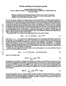
FIG. 3. Contribution coefficients of the state in the spin network basis for some values of the parameter λ. Note that the peak is centered at the fundamental representation.

Thus, using the relations (3.7) the cylindrical function (3.3) expanded on the basis Φj is given by ∞ X X gi (A) = C(λ) (j + 1) j

n=0

λn Hn (2λ) Φj , ( n−j )!( n+j + 1)! 2 2

(3.9)

We would want to evaluate the sum in the index n of the equation (3.9) but it can not be done exactly. Therefore, one is forced to use the definition of Hermite polynomials in its series expansion an evaluate the expression numerically. The coefficients cj are given by cj = C(λ)(j + 1)

∞ X k=0

2k+j

[ 2k+j ] 2

X (−1)m (2k + j)! λ (4λ)2k+j−2m , k!(k + j + 1)! m=0 m!(2k + j − 2m)!

(3.10)

where [ν] denotes the larger integer ≤ ν. A numerical P∞ 2 evaluation of equation (3.10) was performed and shows, with the normalization i=0 cj = 1, that the series converges in the interval 0 < λ < 1 and for values above λ ≥ 0.5 a peak starts to grow at the fundamental representation. Fig. 3 shows some coefficients for some values of λ. It is important to stress out that for larger values of the ’color’ j the expansion continues, but in this case a numerical evaluation turns out to be inappropriate due to float point errors. The most important and intriguing difference between the ‘quasi-coherent’ weave [11] and the ‘Gaussian’ weave is that, in the last case the peak of the coefficients (3.10) in the basis of spin-network states is centered around the fundamental representation j = 1. The dominance of the fundamental representation in other physical situation such as the BH entropy seems to point to a deep role played by the fundamental representation in loop quantum gravity. The origin of this behavior deserves further attention. 11

One can get a closed formula for the expectation value for the area in the state gi using the machinery of recoupling theory [17,19] in the loop representation r XX ˆ = j ( j + 1) hAi c∗k cj h | i. (3.11) 2 2 j k j

k

0

j

0

k

Where the bracket can be evaluated chromatically to show that the basis states are normalized. Thus, the expectation value of the area operator is given by, r X j j ˆ = (8πℓ2P ) ( + 1). (3.12) hAi |cj |2 2 2 j In the case of the volume operator, a closed formula for the expectation value is not available. However, we know that the largest eigenvalue in the state Ψj increase as j 3/2 and we can make an estimation. For the particular value of the Gaussian width λ = 0.75 we have the following expectation values for the geometric operators and their respective dispersions: q 2 ˆ ˆ 2 = 0.432(8πℓ2 ), hAi = 1.149(8πℓP ) ; ∆A := hAˆ2 i − hAi (3.13a) P q ; ∆V := hVˆ 2 i − hVˆ i2 = 2.435(8πℓ2P )3/2 , (3.13b) hVˆ i = 1.078(8πℓ2P )3/2 As expected, the mean values and dispersion of the basic geometric observable are of the order of ℓ2P in the case of the area and of ℓ3P in the case of the volume. Our state gi is peaked in area and volume as in a similar fashion as the proposal given in [11], but with better accuracy. It is easy to see that the state (3.4) satisfies the necessary conditions to be considered a weave state, because the expectation values (3.13) are of the order of suitable powers of the Planck length. For a formal demonstration we refer to [11]. IV. DISCUSSION AND OUTLOOK

In this work we have proposed a basic cylindrical function with a Gaussian dependence on the group element. This function can be used, in particular, to construct a weave state a la Grot-Rovelli. The particular proposal has the desired features of a weave state plus a peakedness property around the fundamental representation. There exists a striking similarity between the main contribution of the state in the fundamental representation and the dominating states, in the statistical counting, that contributes to the entropy of an ‘isolated horizon’. This dominant contribution correspond to punctures all of which have labels in the fundamental representation (spin 1/2) [5]. The Gaussian state proposed here can play an important role both as a background to construct new Hilbert spaces and as a suitable state in the recent proposal for lattice based semi-classical states in loop quantum gravity [6]. We finish by pointing out several issues that deserve further investigation: 12

1. One would like to understand the physical foundations for the fact that there is a dominance of the fundamental representation in at least two different situations. 2. It is necessary to investigate the role played by these (or other) ‘quasi-classical’ states in the recovery of a commutative classical geometry. 3. In the construction of new Hilbert spaces a la GNS, different choices of ‘vacuum states’ might lead to unitarily inequivalent Hilbert spaces. It is important to understand if the Gaussian ansatz presented here yields an equivalent or inequivalent quantum theory to the one constructed in [11]. There are also coherent states constructed using ‘infinite tensor product Hilbert spaces’ [7]. The relation of this method to the algebraic GNS construction remains unclear and deserves further attention. 4. Finally, we would like to understand the relation of the Gaussian ansatz to the coherent states constructed in [7], specially since both are constructed using coherent state-like states on the group. Some of these issues are under investigation and shall be reported elsewhere. ACKNOWLEDGMENTS

We would like to thank S. Gupta and J.A. Zapata for discussions, and a referee for helpful comments. This work was partially funded by DGAPA No. IN121298 and CONACyT No. J32754-E grants. JMR was supported in part by CONACyT scholarship No. 85976.

13

REFERENCES [1] For recent reviews see: C. Rovelli, Loop quantum gravity (1998). Preprint gr-qc/9710008; A. Ashtekar, Quantum Mechanics of Geometry (1999). Preprint gr-qc/9901023. [2] C. Rovelli and L. Smolin, Discreteness of area and volume in quantum gravity, Nucl. Phys. B442, 593-622 (1995); C. Rovelli and L. Smolin, Erratum: Nucl. Phys. B456, 734 (1995). [3] A. Ashtekar and J.Lewandowski, Quantum theory of geometry: I. Area Operators Class. Quant. Grav. 14 A55 (1997); Quantum Theory of Geometry: II. Volume operators Adv. Theor. Math.Phys. 1 388 (1998). [4] A. Ashtekar, A. Corichi and J. A. Zapata, Quantum theory of geometry III: Noncommutativity of Riemannian structures, Class. Quant. Grav. 15, 2955 (1998). [5] A. Ashtekar, J. Baez, A. Corichi and K. Krasnov, Quantum Geometry and Black Hole Entropy, Phys. Rev. Lett. 80, 904 (1998). A. Ashtekar, J. Baez and K. Krasnov, Quantum Geometry of Isolated Horizons and Black Hole Entropy. Adv. Theor. Math. Phys. (in press). Preprint gr-qc/0005126. [6] M. Varadarajan and J. A. Zapata, A proposal for analyzing the classical limit of kinematic loop gravity. Preprint gr-qc/0001040 [7] T. Thiemann, Gauge field theory coherent states (GCS). I: General properties. Preprint hep-th/0005233. [8] A. Ashtekar, C. Rovelli and L. Smolin, Weaving a classical metric with quantum threads, Phys. Rev. Lett. 69, 237 (1992). [9] T. Thiemann, QSD V: Quantum gravity as the natural regulator of matter quantum field theories, Class. Quant. Grav. 15, 1281 (1998). [10] J. Iwasaki and C. Rovelli, Gravitons as embroidery on the weave, Int. J. Mod. Phys. D1, 553 (1993); Gravitons from Loops: non-perturbative loop-space quantum gravity contains the graviton-physics approximation. Class. Quant. Grav. 11, 1653 (1994). [11] M. Arnsdorf and S. Gupta, Loop quantum gravity on non-compact spaces. Nucl. Phys. B577, 529 (2000). [12] N. Grot and C. Rovelli, Weave states in loop quantum gravity, Gen. Rel. and Grav. 29, 1039 (1997). [13] A. M. Perelomov Generalized Coherent States and their Applications, Berlin; N. Y. Springer-Verlag (1986). [14] A. Ashtekar, J. Lewandowski, D. Marolf, J, Mour˜au and T. Thiemann, Quantization of diffeomorphism invariant theories of connections with local degrees of freedom, J. Math. Phys. 36 6456 (1995). [15] A. Ashtekar, New variables for classical and quantum gravity, Phys. Rev. Lett. 57, 2244 (1986). F. Barbero, Real Ashtekar Variables for Lorentzian Signature, Phys. Rev. D51, 5507 (1995). [16] T. Thiemann, Quantum spin dynamics (QSD). VII: Symplectic structures and continuum lattice formulations of gauge field theories. Preprint hep-th/0005232. [17] R. De Pietri and C. Rovelli, Geometry eigenvalues and the scalar product from recoupling theory in loop quantum gravity, Phys. Rev. D 54 4, 2664 (1996). 14

[18] A. Ashtekar, A. Corichi and J. A. Zapata, Notes on the area operator, (1996). Unpublished. [19] L. H. Kauffman and S. L. Lins, Temperley-Lieb Recoupling Theory and Invariant of 3-Manifolds, Princeton University Press, NJ (1994).

15