and Cancellation in Wireless Networks. Li Erran Li ... Interference in traditional wireless networks has been con- ...... Cambridge University Press, May 2005.
A General Algorithm for Interference Alignment and Cancellation in Wireless Networks Li Erran Li , Richard Alimi† , Dawei Shen , Harish Viswanathan and Y. Richard Yang† † Bell Labs MIT Yale University �
�
Abstract—Physical layer techniques have come a long way and can achieve close to Shannon capacity for single pointto-point transmissions. It is apparent that, to further improve network capacity significantly, we have to resort to concurrent transmissions. Multiple concurrent transmission techniques (e.g., zero forcing, interference alignment and distributed MIMO) are proposed in which multiple senders jointly encode signals to multiple receivers so that interference is aligned or canceled and each receiver is able to decode its desired information. In this paper, we formulate the interference alignment and cancellation problem in multi-hop mesh networks. We show that the problem is NP-hard in general. We then propose a convex programming based algorithm to identify interference alignment and cancellation opportunities. Our algorithm effectively utilizes knowledge of both local network topology and overheard packets at the sender side as well as the receiver side. We implement our system using GNU Radio to evaluate key practical implementation issues.
I. I NTRODUCTION Interference in traditional wireless networks has been considered harmful, as supported by both theoretical analysis (e.g., [6]) and experimental measurements (e.g., [8], [9]). The detrimental effects of interference are particularly severe as a traditional wireless network becomes larger. However, as point-to-point link throughput approaches Shannon capacity, it becomes increasingly important to allow simultaneous transmissions in order to substantially improve wireless network capacity. As a result, techniques for achieving simultaneous transmissions and receptions have been a research topic of intense interest. In the communications community (e.g., [1], [12]), novel techniques such as zero forcing [12] and interference alignment [1] are proposed. In these techniques, multiple senders jointly encode signals to multiple receivers such that interfering signals will cancel out, and each receiver is able to decode its desired information. In this paper, we refer to all of these cooperative sender-side techniques as cooperative interference alignment techniques, or interference alignment for short. Receivers can also utilize overheard packets or even exchange received packets through wireline links to cancel interference in order to extract the desired packets. We refer to the receiver-side technique as interference cancellation. Previous investigations on interference alignment and cancellation either target specific opportunities (e.g., [7], [4]) and thus miss beneficial opportunities or are mainly theoretical by focusing on asymptotic behaviors. Specifically, in [10], Niesen, Gupta and Shah show that, in arbitrary extended networks, optimal capacity scaling cannot be achieved using the traditional point-to-point link abstraction for α 3, where �
signal decays with distance to the power of α; cooperative schemes are required to achieve optimal scaling. In [11], Ozgur, Leveque and Tse propose a hierarchical cooperative transmission scheme. They show that, in random extended networks where the area is fixed and the density of nodes increasing, the total capacity of the network scales linearly with the number of nodes n; in random extended networks where the density of nodes is fixed and the area increasing linearly with n, the capacity scales as n2 α 2 for 2 α 3 and n for α 3. In this paper, we seek to design a general algorithm that can identify the best interference alignment and cancellation opportunities in practical settings where a node has only local information. In particular, the local information includes only local topology (one or two hops), and the set of packets that each sender or receiver has. We make the following contributions: �
�
�
�
�
�
We identify diverse, novel scenarios for using interference alignment and cancellation to improve network throughput. We formulate the general problem of optimal interference alignment and study its computational complexity. We show that it is computational challenging (NP-hard). We present a promising, distributed algorithm for identifying a wide range of opportunities for interference alignment and cancellation. The algorithm makes elegant use of channel state, degree of freedom, and opportunistically received packets at both the sender side and the receiver side. �
�
�
To further progress towards making interference alignment practical, we implement our algorithm in GNU radio. We identify two key issues. The first is time synchronization. It is a common assumption in previous studies (e.g., [1], [12], [11]) that transmissions be synchronized. We investigate how difficult it is to meet synchronization requirements in a distributed setting. The second issue is channel estimation. Channel status can be particularly helpful in interference alignment. Can channel estimation be achieved for multiple packet durations? Specifically, for physical-layer implementation of interference alignment, we make the following contributions: �
Leveraging OFDM, we do not need precise time synchronization as long as multiple transmissions are synchronized within an OFDM cyclic prefix. Using implementation in GNU Radio, we show that we can achieve this if the largest propagation delay difference from senders to any receiver
�
�
�x H �
vector transpose). By rewriting the received signal as
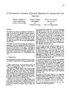
Fig. 1. A 2 antennas.
�
2 MIMO transmission where both sender and receiver have 2
is relatively small. Using GNU Radio, we study the accuracy of channel estimation. In commercial hardware, channel estimates may be more stable; however we have not observed this using GNU Radio. This makes it difficult to achieve interference alignment using opportunistically received packets at the sender side. Interference cancellation at the receiver side is not affected. II. R ELATED W ORK
Although there is a large body of literature on related topics, there are fewer studies on practical systems issues. Our investigation is based on previous interference alignment techniques, including interference cancellation [12], zero forcing [12] and interference alignment [1]. There has been some recent work on practically applying interference alignment and cancellation techniques (e.g., [7], [14], [4]). Katti et al. [7] have proposed ANC (conceptually similar to [14]). ANC exploits interference cancellation opportunities in multi-hop wireless networks. In particular, the 2-hop 3-node line topology and 5-node “X” topology are evaluated using GNU Radio. It is shown that ANC can improve throughput up to 70%. They do not consider zero forcing or interference alignment techniques. Gollakota, Perli and Katabi [4] have designed an interference cancellation and alignment scheme in a specific setting where synchronization is not required. They do not exploit zero-forcing techniques. In addition, their results are only for one-hop wireless networks. III. BACKGROUND : MIMO AS A S PECIAL C ASE I NTERFERENCE A LIGNMENT
�
�
�
�
��� � �
��� �
�
H
1 0
1
0 1
x
2
(1)
we can view the received signal as the sum of two scaled vectors. The decoding of each packet, say x1 , can be viewed as projecting H 1 0 T x1 onto a vector that is orthogonal to the vector H 0 1 T carrying the interfering signal x2 . If the sender knows the channel H, the sender can multiply H 1 with X and send the resulting signal X . Again, ignoring noise, we can verify that receiver antenna 1 will receive only x1 , no mixing of x2 ; similarly, receiver antenna 2 will receive only x2 . This technique is often called zero forcing. The channel inverse is a specific type of encoding vector. This vector view of received signal enables the general technique of interference alignment. Rather than nulling all interference at the receivers like zero forcing, the senders can encode the signals such that interfering signals are aligned in a direction that is different from the desired signal. To decode, the receiver just projects the received signal onto a vector that is orthogonal to the vector of the interfering signal. Although effective in many settings, centralized MIMO has many limitations. In particular, the number of antennas that can be placed on a node to allow independent channels is limited due to the size limitation of communication devices. Thus, it is desirable to extend interference alignment to a distributed setting.
� � � �
�
�
IV. D ESIGN C HALLENGES A general multi-hop wireless network using interference alignment is shown in Figure 2. The general network setting creates substantial challenges. Below, we enumerate two key challenges: (1) limited knowledge of packets at distributed senders and receivers; and (2) degree of freedom constraints.
OF
We use centralized MIMO to illustrate the basic idea of interference alignment. As shown in Figure 1 (see also [4]), a MIMO sender and receiver, each with M antennas, can potentially achieve throughput M times that of using a single antenna, under the same total transmit power constraint. Let’s briefly illustrate how this is achieved when M 2. If we represent the signals corresponding to packets 1 and 2 as x1 , x2 respectively, ignoring noise, we have that the received signals at receiver antennas 1 and 2 are y1 h11 x1 h21 x2 , and y2 h12 x1 h22x2 respectively. Here hi j is a complex number whose magnitude and phase represent signal attenuation and delay from sender antenna i to receiver antenna j. The receiver estimates the channel H as shown in Figure 1. It can recover x1 and x2 by multiplying H 1 , the inverse of H, with the received signal vector Y (Y y1 y2 T where T represents
�
y1 y2
Fig. 2.
Interference alignment in distributed settings.
Limited knowledge of packets at distributed senders and receivers: In a distributed setting, to achieve interference alignment using the preceding MIMO technique, either we need to exchange packets such that all n senders have the same set of packets when computing interference alignment or we need to exchange received samples among receivers. In a no-infrastructure support environment, it is infeasible to exchange received samples. Take a setting where each sender
has 1 antenna on a 20 MHz 802.11 channel. Then the raw sample rate will be 40 Msamples/second. If each sample is represented by 8 bits, it translates into 320 Mbps information for a receiver to send. Although it is possible to exchange packets at the sender side, this introduces substantial overhead. Without exchanging packets (or with limited exchange) and no exchange of received signal in sample form, a distributed interference alignment algorithm is faced with the challenge of effectively utilizing the following identified opportunities: The sender makes use of overheard packets for constructing interference nulling or alignment; The receiver makes use of overheard packets for interference cancellation; The algorithm exploits the channel structure between distributed senders and receivers. That is, due to signal attenuation, sender i may just slightly raise the noise floor of receiver j. In this case, we can set hi j 0.
�
Degree of freedom (DOF) constraints: The number of independent signals that can be produced at a sender is typically referred to as the degree of freedom (DOF) of the sender. Generally, if the channels from a given sender’s antennas to those of the receivers are independent, then the sender with M antennas is said to have M degrees of freedom. The number of independent frequencies is also counted as degree of freedom. For example, 802.11a/g has 48 used data subcarriers. The number of independent subcarriers is the number of degree of freedom that these subcarriers have. It has been shown [1] that, using interference alignment every sender-receiver pair can potential achieve half of its degree of freedom among parallel transmissions. However, the construction for the alignment scheme is by assuming that each sender has many degrees of freedom (e.g., more than 1000 for a 4x4 parallel transmission). In reality, the number of DOF that a sender has is limited. Thus, it is a challenging problem on what the best interference alignment can do with limited degree of freedom. V. D IVERSE S CENARIOS The preceding section identifies two key systematic design challenges. In particular, limited knowledge of packets demands efficient utilization of available packets to construct interference alignment and cancellation. In this section, we show novel, practical scenarios beyond simple scenarios in [7], [4]. In the examples below, each sender has only one degree of freedom. For simplicity, we ignore noise and assume that channels are known to neighboring nodes; we use a simple slotted model to illustrate basic concepts; we assume that there is a triggering mechanism to start concurrent transmissions of multiple transmitters. In each scenario, if there is no edge between a sender and a receiver, then the sender’s transmission causes minimal interference at the receiver and thus can be ignored. In our notation, packet pkti ’s signal is denoted as xi . Helper node with native packets: Traditionally, a node transmits only when it has a packet to its intended receiver. Utilizing interference alignment, a node can transmit even if it
u1
pkt1
s1
d1
u3
pkt2
s2
d2 u2
Fig. 3. A network with two senders and two receivers: a helper node can help two senders.
has no intended receivers. We refer to such a node as a helper. Furthermore, a helper node can help more than one sender. Figure 3 is a simple example to demonstrate the aforementioned benefits. In this example, the existence of a link from one node to another node indicates that the transmissions from the first node can be received by the second one. The traffic in the example is that s1 has pkt1 with final destination d1 through u1 , and s2 has pkt2 with final destination d2 through u2 . Without interference alignment, it takes 4 slots for the two packets to reach their destinations (e.g., s1 to u1 , s2 to u2 , u1 to d1 , and u2 to d2 in slots 1,2,3,4 respectively). With interference alignment, node u3 in the middle can help u1 and u2 to transmit simultaneously. In slot 1, s1 sends to u1 ; in slot 2, s2 sends to u2 ; in slot 3, u1 u2 u3 transmit at the same time. Let hi j be the channel from ui to d j where i 1 2 3 and j 1 2. Then, u3 transmits x3 which is constructed from overheard packets pkt1 and pkt2 in the preceding rounds: h12 h21 x3 h32 x1 h31 x2 . One can verify that for y j at d j , where j 1 2, we have that y j h1 j x1 h2 j x2 h3 j x3 is a scaled version of x j . For example, y1 h11 h31h32h12 x1 ; that is, the interference from the other packet is nullified.
��� �
�
�
�
�
�
� �
� � �
Helper nodes with mixed packets: A helper can help even with only mixed packets. As shown in Figure 4(a), packet pkt1 ’s next hop is u1 and destination is d1 , and packet pkt2 ’s next hop and destination is d2 . If there is no helper, it will take 3 time slots for both packets to arrive at their destinations: s1 to u1 , u1 to d1 and s2 to d2 in slots 1,2,3 respectively. With helper node u2 , it takes only two time slots: in the first slot, both s1 and s2 transmit (s1 ’s transmission does not cause any interference at d2 ); in the second slot, both u1 and u2 transmit. u1 u2 have only a mixed packet (the combined signal of pkt1 and pkt2 ). Let hi j be the channel between si and u j ; gi j be the channel between ui and d j . We can see that ui will receive yi h1i x1 h2i x2 . If u1 sends h22 g21 y1 and u2 sends h21 g11 y2 , then d1 will only receive h21 h12 h11h22 g11 g21 x1 . So far the gains of our examples are no more than 50%. The example in Figure 4(b) shows that we can achieve 100% gains. Without helper nodes v1 and v2 , we need 4 time slots (s1 to u1 , s2 to u2 , u1 to d1 , and u2 to d2 in slots 1,2,3,4 respectively). With helper nodes, we need only 2 slots: in slot 1, both s1 and s2 transmit; in slot 2, u1 , u2 , v1 and v2 , each sends a scaled mixed packet. This results in that d1 receives a scaled version of pkt1 and d2 receives a scaled version of pkt2 . Essentially, v1 nulls the interference component of pkt2 in u1 ’s
�
�
� � �
�
pkt1
s1
u1 pkt1
u2
s1
pkt2
s2
v1 v2
pkt2
s2
d1
d1
u1
pkt2
d1
(a) 1 helper node
s1 pkt1 Fig. 7. A network with two senders and two receivers; local routing creates interference control opportunities.
(b) 2 helper nodes
Fig. 4. Networks with two senders and two receivers: helper nodes have only mixed packets.
mixed packet. Similarly, v2 nulls the interference component of pkt1 in u2 ’s mixed packet. Note that, v1 does not interfere at d2 and v2 does not interfere at d1 . u1 d1 s pkt 1 1
pkt2
s2
u2
d2
Fig. 5. A network with two senders and two receivers: interference alignment and cancellation.
Interference alignment and cancellation: In Figure 5, in a traditional network, it will take four time slots for both d1 and d2 to receive their respective pkt1 and pkt2 from s1 and s2 . With interference alignment and cancellation, s1 and s2 can transmit their respective packets simultaneously in the first slot. Note that, u1 receives a mixed signal. In the second slot, u1 and u2 transmit simultaneously without any particular encoding. d1 can use pkt2 received in the first slot to cancel interference. To implement this scenario, one possibility is that u1 can be a coordinating node to transmit a triggering message. The triggering message instructs s1 s2 to transmit simultaneously, and u1 u2 to send immediately thereafter. The triggering message also informs d1 of its decoding vector.
pkt1
u1
v1
d1
u2
v2
d2
s
pkt2
Fig. 6. A network with two senders and two receivers: multi-hop interference alignment.
Multi-hop interference alignment: It can be beneficial to make interference alignment decisions two hops away from the receivers. Consider the example in Figure 6. Assume that nodes u1 u2 first receive packets pkt1 pkt2 from S in two time slots. Now consider two different transmission strategies. In the first strategy, u1 u2 encode their packets to allow v1 v2 to decode pkt1 , pkt2 respectively. Then v1 and v2 have to transmit in separate time slots to relay the two packets to their destinations. As a result, the first strategy takes a total of 5 slots. To describe the second strategy, let the channel matrix between u1 u2 and v1 v2 be H1 , and between v1 v2 to d1 d2 be H2 . Let the encoding vector at ui be ωi . Let the received signals at d1 d2 be y1 y2 respectively. If we let ω1 ω2 T H2 H1 1 , then y1 y2 T Γ x1 x2 T , where Γ is a
�
� � �
�
�
� � � � �
d2
d2
u2
d2
s2
u1
diagonal matrix. That is, u1 u2 encode pkt1 pkt2 with ω1 ω2 respectively, and transmit simultaneously to v1 v2 in the third slot. In the fourth slot, v1 v2 will amplify their received signals with the same magnitude and transmit at the same time. The second strategy will result in a total of 4 instead of 5 slots.
The need for local-routing: In Figure 7, there are two flows: pkt1 goes from s1 to d1 and pkt2 goes from s2 to d2 . Suppose that the original routing from s1 to d1 is through s2 . Then it will take 3 slots to deliver the two packets: it takes one slot for pkt1 to arrive at s2 ; since s2 cannot send and receive at the same time, it takes s2 one slot to forward pkt1 and one slot to send pkt2 . However, if we reroute the first packet from s2 to u1 , we need only two time slots. In the first slot, both s1 and s2 can send. Both d1 and d2 will receive pkt2 . Then u1 will receive a mixed packet and can just forward the mixed packet. Node d1 can decode pkt1 using the stored packet pkt2 . VI. P ROBLEM F ORMULATION AND C OMPUTATIONAL C OMPLEXITY The preceding section gives concrete examples. In this section, we precisely define the problem to be solved. A. Problem Definition We first state our design assumptions. We assume that a node computes multiple sender transmission opportunities for its neighbors and triggers the transmissions using signaling information piggybacked in either ACK packets or DATA packets. We assume that the node can identify such opportunities using overheard flow information, and channel estimations. We do not assume that head-of-line packets are always transmitted in a concurrent transmission opportunity. A higherlevel mechanism will schedule transmissions to integrate a given fairness objective. We assume that all native packets are linearly independent. Consider a specific node s1 in the wireless network. For ease of description, we consider a single rate network (i.e., all transmissions use the same rate ρ). Node s1 uses local information available at itself to compute interference alignment and cancellation opportunities. The local information consists of overheard packets, exchanged packet identifiers, channel information, a transmission graph G V E , and a interference graph GI V EI , where V consists of nodes in a local neighborhood of s1 (e.g., within two hops away from it in G). An edge e u v means that transmissions with rate ρ are feasible between u and v. If there is no edge between u v
� � � � � �
� � �
in GI , then u’s transmissions will cause negligible interference at v, and vice-versa. Note that our interference graph is nodebased. For simplicity, we assume that all nodes have the same degree of freedom DOF. We assume a set S of senders. We use si to denote sender i. There is also a set R of receivers. We use d j to denote receiver j. Denote the channel matrix between the sender and receivers as H. In the case of DOF 1, we implicitly assume that pkt j ’s receiver is d j . We assume that the set of senders and the set of receivers are disjoint. There may be more senders than receivers. In that case, some senders act as helper nodes. They will transmit overheard packets. Denote the coding coefficient matrix as Φ. The received signals at the receivers can be denoted as Y HΦX Z, where X is the vector of packets, Y the vector of received signals at the receivers, and Z the vector representing noise at the receivers. Note that, if DOF 1, we take a block view of HΦ where each non-diagonal element is a vector of dimension DOF. A diagonal element for receiver d j consists of λ j vectors (each of dimension DOF), where λ j is the number of packets that receiver d j wants to receive from the senders. Ideally, during each time slot, we would like to pack the maximum number of concurrent transmissions at rate ρ. In the best case, we find a Φ such that the non-diagonal elements of HΦ are either zero or aligned in subspaces not containing the diagonal vectors, and all the elements at the diagonal support the given fixed rate. This makes sure that every receiver gets its sender’s packet. However, this may not be always possible. If not possible, we want to find a Φ with a submatrix G of HΦ of maximum size with the following property: non-diagonal elements are either zero or aligned, and diagonal elements are all non-zero. We refer to our problem as the generalized interference alignment and cancellation (GIAC) problem.
�
�
�
B. Computational Complexity As we have shown in the preceding section, there are diverse scenarios where we can apply interference alignment. A natural question to ask is: can we efficiently identify these opportunities? Even for the simple case of DOF=1, we can show that the interference alignment and cancellation problem is NP-hard. The proof is by a reduction from the MAX INDEPENDENT SET problem. Given a graph G V E , the maximum independent set asks for a set B � V with the maximum cardinality �� such that, for any two nodes u v � B, u v � E. Theorem 1: Assume that DOF = 1, and that packets are linearly independent. The general interference alignment and cancellation (GIAC) problem is NP-hard. Proof: Our reduction is from independent set. Given a G V E , we create an instance of GIAC problem as follows. We label the vertices as u1 u2 ������ u � V � . For each ui � V , we create a sender si and receiver di . Only sender si has packet pkti . Let hii 0. For each edge ui u j , we add channels hi j h ji with non-zero values. We see that if there is an edge ui u j in the independent set problem, and si transmits its packet pkti , then s j cannot concurrently transmit pkt j , because the
� � �
� �
� � �
� �
�
�
interference caused by s j at receiver di cannot be forced to zero given that no other nodes have pkt j and all packets are independent. Thus, an independent set in G corresponds to a set of senders in our GIAC problem where simultaneous transmissions can all be decoded correctly at each intended receiver, and vice-versa. Note that, our proof has assumed that arbitrary interference among nodes are possible. We leave the complexity for specific interference models to future work. VII. D ISTRIBUTED A LGORITHMS Given the computational complexity of finding an optimal solution, we focus on designing practical algorithms with sound heuristics. The algorithm we design in this section can find all of the opportunities presented in Section V as well as those presented in [7], [4]. A. Optimal Algorithm for a Special Case There is an optimal algorithm for interference alignment with complete channel matrix and no receiver side information (a receiver has not received any packets from any sender). Specifically, if the elements in the channel coefficient matrix are all non-zero and the matrix has full rank, then the problem can be solved optimally. DOF=1: For simplicity, the algorithm where all nodes have DOF of 1 is shown in Figure 8. We assume that the set of senders and the set of receivers are disjoint. Let S denote the set of senders, and aik whether sender si has pktk . Lines 1-8 are simply finding the maximum set PKT of packets (receivers, since for DOF=1, there is a one-to-one correspondence of packet and receiver) such that each packet pktk � PKT has at least PKT senders. This ensures that there are enough independent equations to zero force pktk at the other unintended receivers. As an example, consider Figure 3 after s1 and s2 transmit. For the next round, the senders are u1 , u2 and u3 ; the receivers are d1 and d2 . Node u1 has packet 1 (to d1 ), u2 has packet 2 (to d2 ), and u3 has both packets. Thus, the packet availability matrix is A
�
�
1 0 0 1 1 1
�
Running lines 1-8 of the algorithm, we identify that each packet has two senders (n1 = n2 = 2). Thus, both packets will be selected for transmission (the while loop is not executed). Lines 10-15 is an optimization to select the minimal number of senders. We use a greedy algorithm to remove redundant senders one by one. We can also replace lines 10-15 by a greedy k-set cover heuristic. Theorem 2: In the case of no receiver side information (no receiver has any packets of any senders), the interference alignment algorithm is optimal if the elements in H are all non-zero and H has full rank. Proof: Sketch. The key insight is that ni 1 represents the number of nodes that can be transmitted simultaneous
�
�
S
1. Let nk ∑i� 1 aik ��� k 1 � 2 ��������� K 2. Order nk such that nπ1 nπ2 � ��� nπK 3. Let PKT be the set of packets to be transmitted 4. Let t 1 5. while � PKT � nπt 6. PKT PKT ��� pktπt � 7. t t� 1 8. endwhile 10.Let T be the subset of S whose packets in PKT 11. Let T � S 12. For any sender si � S � T 13. if remove si from T � , each pkt � PKT still has � PKT � number of senders 14. T� T � ��� si � 15. endfor
��
��
��
y1 y2 y3
��
H11 v1 H12 v1 H13 v1
H41 v4 H42 v4 H43 v4
H21 v2 � H11 v5 H22 v2 � H12 v5 H23 v2 � H13 v5
�
�
�
� �
�
1.
with pkti at sender i. It does not matter which set of nodes. We remove packets one by one if they limit the number of simultaneous transmissions until we reach the optimal. Note that the algorithm assumes that the diagonal elements of HΦ support rate ρ for all senders. In practice, there may be power limitations. We will return to this issue in our general algorithm. DOF 1: We can extend the preceding algorithm to the case of DOF 1. Figure 9 shows an example with four senders and three receivers, where DOFi 2 �� i 1 2 3. In this example, senders s1 , s2 , s3 , s4 have pkt1 , pkt2 , pkt3 , pkt4 respectively. Each sender has a corresponding receiver d1 , d2 , d3 , d1 . Sender s1 overheard pkt2 pkt3 . If DOF is one for all nodes, then we can send only two packets using zero forcing. However, in the case of DOF 2 for all, three packets pkt1 ptk2 pkt3 can be sent through interference alignment [4], [5]. This is because each DOF provides an independent equation to align the two other interfering signals. In this example, with overhearing, we can actually send four packets combining zero forcing and interference alignment. Specifically, s1 encodes pkt1 pkt2 pkt3 with vector v1 v5 v6
� �
�
�
�
� � �
An example case with DOF
H31 v3 � H11 v6 H32 v3 � H12 v6 H33 v3 � H13 v6
�
�
��
��
x1 � x4 x2 x3 (2)
�
Specifically, in the encoding, we zero force the non-diagonal elements of the first row by H21 v2 H11 v5 0 and H31 v3 H11 v6 0. We then align the non-diagonal elements of the second and third row by H12 v1 H42 v4 H32 v3 H12 v6 and H13 v1 H43 v4 H23 v2 H13v5 . Note that for our problem with complete channel matrix and receiver side information (i.e., receivers may have overheard some senders’ packets), we prove that it is still NP-hard. Theorem 3: In the case of receiver side information (a receiver may have packets of other senders a prior, e.g., through overhearing), the general interference alignment and cancellation (GIAC) problem is NP-hard. Proof: Sketch. The reduction is via the clique problem. Given a graph G V E . For each node ui � V , we create a sender si with packet pkti , and we also create an intended receiver di . For each edge ui u j in E, we let di has pkt j and d j has pkti . Two senders si s j can transmit simultaneously iff edge ui u j � E. A clique of size m corresponds to a set of m senders whose packets can be transmitted simultaneously.
�
Fig. 8. An optimal algorithm for interference alignment with complete channel matrix, no side information, and DOF = 1 for all senders.
Fig. 9.
respectively; s2 s3 encodes pkt2 pkt3 with vector v2 v3 respectively; s4 encodes pkt4 with v4 . Equation (2) shows the encoding, where Hi j denotes the 2 by 2 channel matrix from sender si to receiver d j .
�
�
�
� �
The key intuition why the receiver side is different from the sender side is as follows. A packet pkti at the sender side (say with s j ) provides one independent equation that can null interference of si ’s transmission of pkti at any receiver; this is not the case at the receiver side. A packet pkti at receiver d j can be used to only null interference of pkti at itself. With receiver side information, we need to modify the interference alignment algorithm. For each receiver d j and each packet it has, say pktk , we create a pseudo sender sk j . This pseudo sender has a unit channel coefficient with d j and a zero channel coefficient with all of the other receivers. We defer the algorithm to the general one-hop case. B. Greedy Algorithm for General One-Hop Case The preceding discussion leads naturally to a greedy algorithm for the general case. DOF=1: Again, we first look at the simpler version when DOF is 1 for all nodes. In the preceding algorithm, we compute nk as the number of senders with pktk . The semantics of nk is the maximum number of receivers who can receive their own packets even if pktk is transmitted. Since the channel matrix is complete, nk is computed as we previously defined. In the general case when the channel matrix is incomplete, the senders of pktk may not create any interference at some receivers. Thus, we need to modify the computation of nk . For each packet, we first find the maximum matching between the
1. 2. 3. 4. 5. 6. 7. 8.
Let PKT be the set of packets to be transmitted Add a pseudo sender for any packet pkt � PKT a receiver has while CanNotXmitS(PKT, ρ) nk maxNonIntR PKT � k � � k 1 � 2 ��������� � PKT � Let pkt be the one with minimal � nk � k 1 � 2 ����� � � � K � � PKT PKT ��� pkt � done Prune senders one by one while CanNotXmitS PKT � ρ false �
�
Fig. 10. General algorithm for interference alignment with side information in the one-hop case.
senders who has pktk and the set of receivers (receiver dk must be in the matching). Let the size be mk . We then find the set of receivers which are not interfered by the set of senders in the matching. Let the size of this set be lk . Then nk mk lk . An an example, if sender sk ’s does not create any interference at any receiver and no other senders have the packet, then mk 1 and lk K 1. Line 4 in Figure 10 uses the function maxNonIntR to compute nk according to this revised definition. At the end of the general algorithm, we need to test whether a set of packets can be transmitted simultaneously at a given rate. Let H be the channel matrix (including helper nodes and pseudo senders). Let Φ be the coding coefficient matrix. If there is a feasible solution such that HΦ has only non-zero diagonal elements, then the set of packets can be transmitted simultaneously. This can be solved by convex programming and a gradient method. This is done in Function CanNotXmitS PKT ρ in Figure 10. We now present its formulation. Let W w1 w2 ������ wK .
�
�
�
�
� �
� � �
�
minimize
� ��
f W
K
∑ wi ρ
i 1 �
K
� � where f W
∑ wi
i 1
� 1
(3)
�
maximize
� � � ∑ w BW log 1 h� N K
2
i
2
�
i � �
1
�� j 1 i j �
�
i �
M:
H �
�
i
ii
i 1
K: K
��
��
HΦ hi j 0
∑ φi j 2
j 1
�
An example illustrating the general algorithm: one-hop case.
�
�
�
�
pkt1 , we have L1 1. Thus, n1 M1 L1 3. Similarly, n2 n3 3. Thus, all three packets can be transmitted at the same time. DOF 1: To extend to the case of DOF greater than 1, all we need to change is the following. In Equation (4), if nk is smaller than the cardinality of� the current set of packets PKT , we do not set hi j 0 for all i j. Instead, we replace PKT nk of them with interference alignment equations (IAE). If the total number of DOF is not enough, then we know line 3 will be true and we do not need to explicitly solve the convex programming problem. If receivers are allowed to exchange decoded packets, after we know that a receiver j can decode its packet pktk with enough equation in the IAE step, we can assume that pktk is aligned at an interfering receiver j without consuming DOF. Note that, we can also extend to the case where a sender wants to send more than one packets. All we need to take care of is that the interference alignment at its receiver will have less dimension to operate.
� �
��
�
�
Extension to two-hop and rerouting case The one-hop case algorithm can be easily modified for the two-hop and rerouting case. The main differences are (1) we have to compute twohop matching when we compute maxNonIntR PKT k ; (2) the channel matrix H will be a product of the first hop and secondhop channel matrices H1 , H2 ; (3) we need to deal with helper nodes with mixed packets. We pick the minimal ni . If there is a helper node u one hop away from receiver di that receives � a mixed signal containing pkt j � PKT j i, then we increase ni by one. Once u is picked as a helper for a certain packet, it cannot be chosen for another packet in the case of DOF 1. We do this iteratively until we cannot increase ni . We do not go beyond more than two-hops as it can be challenging in practice to keep channel information up-to-date in such cases.
�
�
is solved by the following convex program:
� � f W �
Fig. 11.
�
�
�
P
�
(4) Equation (3) can be solved by a simple gradient approach where the largest rate among all sender-receiver pairs decreases its weight whereas the smallest increases its corresponding amount. Figure 11 illustrates how maxNonIntR is calculated. In this example, there are three packets. The figure shows the matching step of pkt1 (the red packet) with maximum matching M1 of size 2. Since d3 is not interfered by the transmission of
VIII. I MPLEMENTING A LIGNMENT IN P HYSICAL L AYER AND MAC The preceding section presents our general algorithm. To achieve the benefits of the algorithm, it is essential to evaluate the possibility of implementing distributed interference alignment and cancellation in real settings. Implementing interference alignment requires two important functionalities in the physical layer. First, multiple transmitters must be able to start transmitting signals simultaneously using distributed algorithms. Second, transmitters must obtain the
�
�
�
�
of channel reciprocity. If the sender has the channel estimation for the reverse channel, it can get the estimation for the forward channel. Techniques such as quantization (e.g., [13]) may also be useful to compress the transmitted estimations, but further analysis and experimentation is needed to identify how much quantization is tolerable in practical settings. Since channels can change within 5 to a few hundred milliseconds, the estimations need to be exchange frequently. In our implementation, the complexity for channel estimation over the hardware devices is obtaining channel phase offset estimations, as it is necessary to know the true channel phase offset to perform the encoding. Since estimating the channel’s phase offset is sensitive to the frequency offset between transmitter and receiver, we implement frequency offset correction at the transmitter using a numerically-controlled oscillator (NCO) running at the frequency offset obtained by the receiver. IX. E VALUATIONS Our implementation is based upon the GNU Radio OFDM implementation. Our experiment uses a 512-point FFT with 200 occupied subcarriers, each modulated using BPSK. The cyclic prefix is 128 samples, and the sampling rate is set to 500KHz. This setup produces an overall bit rate of 156.25 Kbps. A. Time Synchronization The first functionality we require is time sychronization between nodes. The basic requirement is that a set of nodes must be able to start transmitting simultaneously when using interference alignment. 1690
Timing offset between TX and RX (samples)
channel state information so they can perform the necessary encoding for interference alignment. We outline the issues we faced, our solutions, and areas that require further improvement. Coordination: Interference alignments have to be coordinated. Without coordination, interference does not get zeroed or aligned, then it will be difficult to decode. To coordinate transmission, we use an appropriate triggering node that identifies opportunities and sends a control message with an encoding vector for each sender, and decoding vector for each receiver. Clock Synchronization: Interference alignment requires that signals from interfering senders align at the receivers. This in general requires synchronization at the sender side. With OFDM, precise synchronization is not required. However, the signals from different senders must arrive within the cyclic prefix of the desired signal at each receiver. In our implementation, the local time maintained by each node is a counter of the samples sent to the USRP (0-valued samples are sent to the USRP when there is no packet). This allows a simple clock to be maintained in userspace with the accuracy of the USRP master clock. Each node maintains the time offset to each of its neighbors. The sending time is encoded in each packet, allowing receivers to update their time offset to the sender. Let ∆i j denote the time offset between sender ui and receiver d j . When beginning interference alignment transmission, the triggering node includes a time t j at a reference node at which the transmission is to begin. Next, each sender ui computes its local time at which it should start the transmission as ti ∆ i j t j . Node i begins sending the first sample of the packet when its counter reaches ti . Carrier Frequency Correction: Practical oscillators cannot generate or sample signals at the precise carrier frequency. There is a frequency offset. Each sender needs to correct this offset when transmitting the signal. Otherwise, the vector representation of each sender’s signal will rotate an angle proportional to the sender’s frequency offset at the receiver. Because the frequency offset is different at different senders, this will destroy the interference nulling or alignment effect. Thus, frequency offset must be corrected to sufficient accuracy so that residual error creates insignificant interference at each receiver. Channel Estimation: Senders need to know the channel to interfering receivers in order to encode its signal such that zero forcing or interference alignment can be achieved. How can we obtain these channel estimates? In 802.11a/g, there are 48 data subcarriers. They are divided into 4 groups. We need at least 4 channel estimations, one for each group. Each channel estimate can be represented as two 32-bit numbers (4 bytes). So for a M M transmission, the total number of channel estimates that need to be exchanged can be 16M 2 bytes. Even for one byte channel representation, the total bytes will be 4M 2 . As we said, we can cut the number of channels needed by ignoring certain channels. One can also make use
1680
1670
1660
1650
1640
1630
0
Fig. 12.
10
20
30
40 Time (s)
50
60
70
80
Timing offset between sender and receiver.
To accomplish interference alignment, we must first ensure that timing offsets can be estimated accurately. Figure 12 shows the drift in time offset as one node transmits to another node over a period of 72 seconds. In this experiment, the transmitter sends 1 packet every 0.5 seconds, and we report the time offset computed by the receiver. The drift is steady at 0.75 samples per second (i.e., a drift of 1.5 microsecond per second). The required update frequency depends on the duration of the cyclic prefix. For example, 802.11a/g has a 0.8 microsecond cyclic prefix. Note that relative node placement between transmitters and receivers also affects this requirement, as propagation delays can become significant for large variations in distances (e.g., light travels about 240 meters in
0.8 microseconds). In particular, the requirement may be more strict depending on distance between nodes and to what degree node distances are known or estimated. B. Channel Estimation
X. C ONCLUSION
Next we evaluate channel estimation, in particular frequency offset. Total Freq. Offset (Hz)
4700 4690 4680 4670 4660 4650 4640 4630 10
Fig. 13.
10.5
11
11.5
12
Time (s) Measured frequency offset between sender and receiver.
Residual Freq. Offset (Hz)
Using our implementation, we can observe how the measured frequency offset varies with time. Figure 13 shows the offset between sender and receiver for a particular 2-second interval. In this experiment, we continuously send packets from the sender to receiver, and record the frequency offset computed at the receiver. We observe that the frequency offset can vary within a 15-20 Hz range very quickly. 50 45 40 35 30 25 20 15 10 5 0 200
Fig. 14.
Thus, the challenge to operating this system using the hardware devices is coping with frequency offset estimation errors to obtain the channel’s true phase offset. AND FUTURE WORK
Interference alignment involving sender cooperation can provide ample throughput gains in wireless mesh networks. We explore the challenges involved. We present a distributed algorithm that can systematically compute the opportunities in a local neighborhood of a node. Given that interference alignment also requires time synchronization and accurate channel feedback, we implement in GNU Radio to study feasibility. We find that time synchronization can be done accurately enough, if the propagation delay difference from senders to any receiver is small compared with the duration of cyclic prefix when using OFDM. However, due to delays in software processing, accurate channel feedback appears to require hardware support. For our future work, we are investigating more powerful methods [2], [3] to achieve interference alignment. We intend to incorporate them in our algorithm. We are exploring another software radio platform with more hardware support. We would like to fully implement our distributed algorithm and design a full-fledged triggering MAC protocol in this platform. We then would like to evaluate our opportunistic interference alignment framework using a larger testbed. R EFERENCES
220
240
260
280
300
Time (s) Residual frequency offset after transmitter-side correction.
Next, to understand the possible effects on interference alignment transmissions, we enable transmitter-side correction of the frequency offset using the last estimate fed back from the receiver. Figure 14 plots the results. We can observe that the residual frequency offset computed by the receiver can still be high. Using transmitter-side frequency offset correction with an inaccurate frequency offset estimate can cause the estimated channel phase to rotate with time. The NCO runs at the frequency offset estimate, to counter the frequency offset between the sender and receiver. The inaccurate frequency estimate causes the NCO to accumulate a phase error over time. To put the previous figure in perspective, we compute a simple example. With a frequency offset estimate error of only 2 Hz, the phase error will be about π4 after 60ms. The total time for setting up the interference alignment transmission in our implementation is larger than 60 ms. As we can observe from the figures above, the implementation is currently not able to achieve a frequency offset accuracy under 2 Hz.
[1] V. R. Cadambe and S. A. Jafar. Interference alignment and the degrees of freedom for the k user interference channel. IEEE Transactions on Information Theory, 54(8):3425–3441, 2008. [2] S. Changho and D. Tse. Interference alignment for cellular networks. In Proceedings of the 42nd Annual Allerton Conference on Communication, Control, and Computing, 2008. [3] S. W. Choi, S. A. Jafar, and S.-Y. Chung. On the beamforming design for efficient interference alignment. CoRR, abs/0906.3737, 2009. [4] S. Gollakota, S. D. Perli, and D. Katabi. Interference alignment and cancellation. In Proceedings of ACM SIGCOMM, 2009. [5] K. S. Gomadam, V. R. Cadambe, and S. A. Jafar. Approaching the capacity of wireless networks through distributed interference alignment. In Proceedings of IEEE GLOBECOM, 2008. [6] P. Gupta and P. R. Kumar. The capacity of wireless networks. IEEE Transactions on Information Theory, 46(2):388–404, Jan. 2001. [7] S. Katti, S. Gollakota, and D. Katabi. Embracing wireless interference: Analog network coding. In Proceedings of ACM SIGCOMM, 2007. [8] J. Li, C. Blake, D. S. J. D. Couto, H. I. Lee, and R. Morris. Capacity of ad hoc wireless networks. In Proceedings of ACM MOBICOM, 2001. [9] Y. Li et. al. Effects of interference on wireless mesh networks: Pathologies and a preliminary solution. In Proceedings of HotNets, 2007. [10] U. Niesen, P. Gupta, and D. Shah. On capacity scaling in arbitrary wireless networks. IEEE Transactions on Information Theory, 55(9):3959– 398, 2009. [11] A. Ozgur, O. Leveque, and D. Tse. Hierarchical cooperation achieves optimal capacity scaling in ad hoc networks. IEEE Transactions on Information Theory, 2007. [12] D. Tse and P. Viswanath. Fundamentals of Wireless Communication. Cambridge University Press, May 2005. [13] G. R. Woo, P. Kheradpour, D. Shen, and D. Katabi. Beyond the bits: Cooperative packet recovery using physical layer information. In Proceedings of ACM MOBICOM, 2007. [14] S. Zhang, S. C. Liew, and P. P. Lam. Hot topic: physical-layer network coding. In Proceedings of ACM MOBICOM, 2006