where each separate tracker outputs a probability density function of the ... The combination may consist of different trackers that track a common object, as well ...
International Journal of Computer Vision 67(3), 343–363, 2006 c 2006 Springer-Science + Business Media, Inc. Manufactured in The Netherlands. � DOI: 10.1007/s11263-006-5568-2
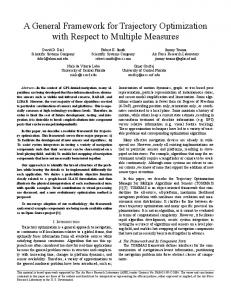
A General Framework for Combining Visual Trackers – The “Black Boxes” Approach IDO LEICHTER∗ , MICHAEL LINDENBAUM AND EHUD RIVLIN Department of Computer Science, Technion – Israel Institute of Technology, Technion City, Haifa 32000, Israel {idol,mic,ehudr}@cs.technion.ac.il
Received December 29, 2004; Revised October 18, 2005; Accepted October 18, 2005 First online version published in March, 2006
Abstract. Over the past few years researchers have been investigating the enhancement of visual tracking performance by devising trackers that simultaneously make use of several different features. In this paper we investigate the combination of synchronous visual trackers that use different features while treating the trackers as “black boxes”. That is, instead of fusing the usage of the different types of data as has been performed in previous work, the combination here is allowed to use only the trackers’ output estimates, which may be modified before their propagation to the next time step. We propose a probabilistic framework for combining multiple synchronous trackers, where each separate tracker outputs a probability density function of the tracked state, sequentially for each image. The trackers may output either an explicit probability density function, or a sample-set of it via CONDENSATION. Unlike previous tracker combinations, the proposed framework is fairly general and allows the combination of any set of trackers of this kind, even in different state-spaces of different dimensionality, under a few reasonable assumptions. The combination may consist of different trackers that track a common object, as well as trackers that track separate, albeit related objects, thus improving the tracking performance of each object. The benefits of merely using the final estimates of the separate trackers in the combination are twofold. Firstly, the framework for the combination is fairly general and may be easily used from the software aspects. Secondly, the combination may be performed in a distributed setting, where each separate tracker runs on a different site and uses different data, while avoiding the need to share the data. The suggested framework was successfully tested using various state-spaces and datasets, demonstrating that fusing the trackers’ final distribution estimates may indeed be applicable. Keywords: 1.
visual tracking, tracker combination, Kalman filter, CONDENSATION
Introduction
Over the past few years researchers have been investigating the enhancement of visual tracking performance by devising trackers that simultaneously make use of several different features. In some cases the feature combination is performed explicitly in a single tracker, usually in the observation phase, whereas in other cases the feature combination is performed implicitly by combining trackers that use different features. ∗ To
whom correspondence should be addressed.
Examples of the first kind may include (P´erez et al., 2002; and Okuma et al., 2004), where better tracking performance was gained by using color histograms in several regions, each of a different part of the tracked object. Further robustness was achieved in (P´erez et al., 2002) by also incorporating the histogram of the background as an additional feature. In (P´erez et al., 2004) color is fused with either stereo sound, for tele-conferencing, or with motion, for surveillance with a still camera. In (Vermaak et al., 2003) three different color bands (RGB) were used together in the observation model. In (Okuma et al., 2004) a particle
344
Leichter et al.
filter, in which cascaded Adaboost detections (Viola and Jones, 2001) are used to generate the proposal distribution and color histograms are used for the likelihood, is used to track hockey players. In (Isard and MacCormick, 2001) the responses of different filters were used together to model the observation likelihood. Another related work is (Collins and Liu, 2003), where the tracker performs on-line switching between different features, according to their quality of discrimination between object and background pixels. An example of the second kind of combination is (Toyama and Hager, 1995), where multiple windowbased trackers simultaneously track the same feature. Different situations in which miss-tracking occurs are categorized and dealt with by the appropriate trackers. In (Gil et al., 1996) the individual estimates of two tracking systems, based on the bounding-box and the 2D pattern of the targets, are combined to produce a global estimate for vehicle tracking. The combination is performed by utilizing instantaneous performance coefficients. In (Shearer et al., 2001) two trackers, a region tracker and an edge tracker, are run in parallel. The two trackers, having complementary failure modes, correct each other based on their confidence measures. In (McCane et al., 2002) the results of two corner trackers, global correspondence and local relaxation, are merged using a classification-based approach and reliability attributes for each corner match. In (Siebel and Maybank, 2002) a system containing three co-operating detection and tracking modules is devised for tracking people in an indoor environment. The three modules are an active shape tracker, a region tracker featuring region splitting and merging for multiple hypotheses matching, and a head detector to aid in the initialization of tracks. In (Darrell et al., 2000) three different modules, which are guided by an integration module using the report of each module, are combined to track people. One module uses stereo data for range computation, another uses color data for skin color localization, and the third is a face pattern detection module. In (Spengler and Schiele, 2003) the so-called democratic integration scheme (Triesch and Malsburg, 2000) was used to combine multiple cues for visual tracking. Two co-inference tracking algorithms, combining trackers of different modalities were developed in (Wu and Huang, 2004). The first co-inference algorithm, combining importance sampling-based trackers, uses the state PDF of each tracker as the importance function for the other tracker. The second co-inference algorithm uses the state PDF of one tracker as the im-
portance function for the other tracker, and then the former tracker uses the latter tracker’s state PDF to compute its own state PDF and observation model parameters through an EM framework. We consider here a general methodology for the combination of synchronous trackers (synchronous in the sense that all trackers receive their frames at the same time instances.) The previous work described above focuses either on feature combination within the tracker, or on a combination of trackers carried out in a specific method tailored to the particular trackers considered. For example, the combination in (Siebel and Maybank, 2002) consists of running multiple trackers in parallel, where each one is devised for a specific sub-task and is dependent on the output of other algorithms for initialization or correction. The trackers described in (Shearer et al., 2001) run in parallel, and switching between their outputs is done according to ad-hoc rules. Perhaps the closest work to our approach is (Spengler and Schiele, 2003), where multiple trackers are run in parallel to track the same object and provide 2D-location distribution estimates, which are combined heuristically by weighted sum. Unlike previous work, the approach presented here is general and not specific to the particular separate trackers used. The separate trackers are treated as “black boxes”, and only their output, which may be modified before their propagation to the next time step, are used. Consequently, the developed framework is fairly general, making it suitable for combining a wide range of trackers in a simple manner. These trackers may even be of different state-spaces of different dimensionality. Since only the separate trackers’ final estimates are used, a second gained advantage is that the combination may be performed in a distributed setting, where each separate tracker runs on a different site and uses different data, while exchanging only their final state PDF (Probability Density Function) estimates and avoiding the need to share the data, which is typically much larger in size (e.g., as in (Blatt and Hero, 2004)). The suggested framework enables tracking enhancement not only by using several sources of data associated with one object, but also by tracking different, related objects (as in the context of the Constrained Joined Likelihood Filter (CJLF) in (Rasmussen and Hager, 2001), where linked objects are tracked with constraints.) Although the simultaneous tracking of multiple objects is a widely approached topic (e.g., (MacCormick and Blake, 2000; Hue et al., 2001; Sidenbladh and Wirkander, 2003)
A General Framework for Combining Visual Trackers – The “Black Boxes” Approach
and many other papers in (Proceedings of the 2001, 2003 IEEE Workshop on Multi-Object Tracking)), it has been approached mainly in the context of independently moving objects. We would like to stress the black box constraint to which our framework is subject, which prevents the use of other data combination methods that are more exact (e.g., Bar-Shalom et al., 1988; Bar-Shalom 1992; P´erez et al., 2002; P´erez et al., 2004; Isard and MacCormick, 2001; Wu and Huang, 2004.) In particular, in the general context of data combination, message passing schemes in the field of graphical models may be an elegant framework for the combination of different data (e.g., Beal et al., 2003; Sudderth et al., 2003; Isard, 2003.) We start by defining the context in Section 2. Then we describe methods to combine explicit PDF-yielding trackers in Section 3, beginning with the case of a common state-space, and continuing with combining trackers using different state-spaces. We show how to combine CONDENSATION-based trackers in Section 4. The combination of explicit PDF-yielding trackers with CONDENSATION-based ones is considered in Section 5. In Section 6 we show how the framework may be used to combine trackers of different, related objects. We continue by presenting experimental results in Section 7, and conclude with a summary and discussion in Section 8. Different parts of this paper were presented in the related papers (Leichter et al., 2004a) and (Leichter et al., 2004b). 2.
propagation to the next time step. A specific tracker outputs either an explicit PDF, or a sample-set of it via CONDENSATION. Such trackers are very common. For example, any tracker using Kalman filtering explicitly provides a Gaussian PDF (namely, a mean vector and covariance matrix) of the tracked state (e.g., (Blake et al., 1993)). Other trackers employing a general discrete probability distribution for tracking are described in (Rosenberg and Werman, 1997a; Rosenberg and Werman, 1997b and Baker and Strens, 1998). Trackers providing samples from general PDFs using CONDENSATION are also widely used. Further on in the paper, we distinguish between explicit PDF-yielding trackers and CONDENSATION-based trackers that provide samplesets from the state PDF. 3) The trackers are conditionally independent, i.e., each tracker relies on features that, given the tracked state, are conditionally independent of the features used by the other trackers. That is, if at time t tracker Ti uses features zit and tracker Tj uses feaj tures zt (i �= j), then we assume that for every state at time t, xt , � � � � � � j j p zit , zt | xt = p zit | xt · p zt | xt .
1) The trackers are black boxes; only their final estimates are observed and may be changed before their back feeding for propagation to the next time step. Note that due to this black box constraint, the inner states and all the modeling used by the trackers, which includes their observation processes and the tracked state’s dynamic model, are hidden. 2) The trackers provide a PDF estimate representation of the tracked state, sequentially for each image, and these PDF estimates may be modified before their
(1)
While this assumption is indeed difficult to verify, there are many cases where it is true or approximately true. Moreover, tracker combination in general is most beneficial when the separate trackers use conditionally independent features in the first place. Therefore, such a conditional independence assumption has been made also in many other visual tracking-related papers (e.g., P´erez et al., 2004; Okuma et al., 2004; Vermaak et al., 2003; P´erez et al., 2002; Darrell et al., 2000; Jepson et al., 2001). Nevertheless, there are tracker combinations that do not rely on this assumption, such as (Wu and Huang, 2004).
Context
We consider the following task: given two or more synchronous trackers (synchronous in the sense that all trackers receive their frames at the same time instances), we would like to combine their outputs into one estimate. The trackers may track a common state or different, albeit related, states. We assume the following regarding the separate trackers:
345
For clearer presentation we will discuss combining two trackers, but the entire discussion and results may be easily generalized for an arbitrary number of trackers. 3. 3.1.
Combining Explicit PDF-Yielding Trackers Same state-space
Let T1 and T2 be two conditionally independent trackers, tracking an object in a common state-space.
346
Leichter et al.
Figure 1. Two separate, explicit PDF-yielding trackers. Both trackers track in the same state-space.
Denote by zit the features extracted by Ti in the tth frame � (t = 0, 1, 2, . . .), and denote by Zit = {ziτ }tτ =0 the feath tures extracted � all frames up to the t frame. � by Tii from At time t p xt−1 |Zt−1 – the tracked state PDF at time t−1, and It – the frame at time t, are available to each tracker as its input. Each tracker Ti extracts� from the � frame its relevant features zit and outputs p xt | Zit – the PDF of the tracked state at time t, given the features zit in the tth frame and all the previously extracted features as well. The overall system of the two separate trackers is illustrated in Fig. 1. � � � Now, using the notation Zt = Z1t , Z2t , let us derive p (xt | Zt ) – the state PDF of the combined system. In the derivation we apply Bayes’ rule (Papoulis 1991) and assumption (1), assumed valid also when given past observations. So,
on time t beginning from t = 0, it is now easily seen that T1 and T2 may be combined by� multiplying �their output PDFs (which will become p xt | z1t , Zt−1 and � � 2 p xt | zt , Zt−1 , respectively), dividing by the PDF p (xt | Zt−1 ), and scaling to have a unit integral. The PDF p (xt | Zt−1 ) in the denominator of (3) is usually referred to as the prediction, or prior PDF – the PDF of the tracked state predicted for the time when the t−th frame is taken, but prior to the measurements in this frame. This PDF may be determined by the tracked object dynamics p (xt | xt−1 ) and the posterior at the previous time, p (xt−1 | Zt−1 ). When combining the trackers, the optimal choice would be to estimate this PDF according to the tracked object dynamics in a separate module. Alternatively, it is common for the separate trackers to have a prediction phase in which the prior PDF is estimated (e.g., a Kalman filter or a general distribution filter (Rosenberg and Werman, 1997a)). If there is access to this already-computed PDF, it may be simply taken from there. However, this option cannot be accomplished under �the black boxes � constraint, where only p xt | zit , Zt−1 are available. In order to obtain the combined estimate, the PDF in the denominator of (3) has to be set in a way that the black box constraint is satisfied, that is, without assuming any knowledge regarding the dynamic model. Clearly, in typical situations visual tracking may be performed even if the dynamic model is not exactly known. Since some dynamic model must be assumed in order to carry on with the tracking, usually a wide PDF
� � p (xt | Zt ) = p xt | z1t , z2t , Zt−1 � � p z1t , z2t | xt , Zt−1 p (xt | Zt−1 ) � � = p z1t , z2t | Zt−1 � � � � = p z1t | xt , Zt−1 · p z2t | xt , Zt−1 ·
p (xt | Zt−1 ) � � (2) p z1t , z2t | Zt−1 � � � � � � � � p xt | z1t , Zt−1 p z1t | Zt−1 p xt | z2t , Zt−1 p z2t | Zt−1 p (xt | Zt−1 ) � � = p (xt | Zt−1 ) p (xt | Zt−1 ) p z1t , z2t | Zt−1 � � � � � � � � p xt | z1t , Zt−1 p z1t | Zt−1 p xt | z2t , Zt−1 p z2t | Zt−1 � � = . p (xt | Zt−1 ) p z1t , z2t | Zt−1
This expression can be written as the product � � � � p xt | z1t , Zt−1 p xt | z2t , Zt−1 p (xt | Zt ) = k · , p (xt | Zt−1 ) (3) where k is the normalization constant independent of x, ensuring the PDF has a unit integral. By induction
is used as the dynamic model. We chose to make the worst case assumption that no knowledge regarding the tracked object dynamics is given in the combination. (The separate trackers, however, do use motion models.) This leads directly to the independency between the current state and previous observations. Thus, we
A General Framework for Combining Visual Trackers – The “Black Boxes” Approach
347
will, however, imply some violation of the black box constraint, and as we saw in our experiments, was not necessary. Trackers T1 and T2 might, for example, be Kalman filters. In this case, if we approximate the pseudo-prior of (3) as Gaussian, then the combined PDF remains Gaussian N(µ,C), with the covariance matrix and mean being C −1 � C1−1 + C2−1 − C3−1 µ � C(C1−1 µ1 + C2−1 µ2 − C3−1 µ3 ), Figure 2. Combining T1 and T2 of Fig. 1: two explicit PDFyielding trackers that use a common state-space.
set the prior in the denominator of (3) to a pseudo-prior that is constant in time, p (xt | Zt−1 ) ≡ p(x),
(4)
which allows us to treat the separate trackers as black boxes. The combined system is illustrated in Fig. 2. Since we would also like to assume that any state that is contained in the image domain is of equal, or approximately equal, probability when no data is given, the static PDF in the right-hand-side of (4) should be set to be uniform or very wide with respect to the image size. Note that the exact combined state PDF (not restricted by the black box constraint and thus may use the true dynamic model) is proportional to the product of the prior and the observation likelihoods (see third line in (2)), where the former is moved to the denominator after manipulations. Thus, using a static, uniform PDF as the pseudo-prior in the denominator of (3) is equivalent to replacing the true prior by its square, which does not change the qualitative effect of the prior on the resulting state estimate: we multiply by a high value for the same states weighted higher by the true prior. We found that this inaccuracy did not come to fruition in our experiments. Perhaps a more accurate alternative to assumption (4) would be to set the pseudo-prior in the denominator of (3) to a diffused version of the posterior at the previous time, p (xt−1 | Zt−1 ). This corresponds to assuming some sort of a general dynamic model in the combination, e.g., a zero-mean Gaussian with a diagonal covariance matrix as the evolution PDF. This
(5)
where N (µ1 , C1 ) and N (µ2 , C2 ) are the PDFs provided by the separate trackers, and N (µ3 , C3 ) is the prior PDF (Bar-Shalom, 1992) (see alternative proof in the Appendix.) Being Gaussian, the combined PDF may be fed back into T1 and T2 . Note that setting the pseudo-prior in the denominator of (3) to be of very high variances is realized here by setting the variances in C3 to be very large. This ensures that C may become non-positive only in the extreme case where both separate trackers provide estimates of very high variances, that is, when both trackers have lost the target. Note also that if desired, the pseudoprior in the denominator of (3) may be brought to the uniform distribution by letting C3 approach the identity matrix scaled by a large factor. Then C3−1 approaches the zero matrix, making the combined PDF N (µ, C) independent of the pseudo-prior in the denominator of (3), as expected. In case the probability distributions are discrete and compact (or may be approximated as such), T1 and T2 may be general distribution filters (Rosenberg and Werman, 1997a).
3.2.
Different state-spaces
Often we can construct conditionally independent trackers in different state-spaces, and then would like to combine them to enhance the tracking performance. This is indeed possible (if the state-spaces are related). In order to combine the trackers we require that a probability distribution on each state-space, conditioned on the state in any of the other state-spaces, is available. In other words, if we denote the state-space of tracker Ti by Si , then for all i �= j, the conditional PDF p(x j | xi ) where xi ∈ Si and x j ∈ S j has to be given. Since this PDF will be used for translating the PDF from the source state-space S i into the target state-space S j , we
348
Leichter et al.
Figure 3. Two separate, explicit PDF-yielding trackers whose state-spaces differ.
denote it by the special name translator and notate it as pSi →S j (x j | xi ). Note that these translators mediate only between the state-spaces and have no connection to the separate trackers. That is, when combining the trackers, the translators only deal with ‘what’ is being tracked and not ‘how’ it is tracked. Thus, in this respect their usage does not violate the black box constraint. We turn now to obtain the combination of T1 and T2 , two conditionally independent trackers, tracking an object in different state-spaces with variables at time t xt and yt , respectively. Denote by S1 and S2 the corresponding spaces, and denote by z1t and z2t the features used in time t by T1 and T2 , respectively. The overall system of the two separate trackers is illustrated in Fig. 3. In order to combine the trackers’ estimations, each provided PDF has to be translated into a PDF in the state-space of the other tracker. This may be accomplished given the translators: the PDFs of the state in one space given the state in the other space – pS2 →S1 (x | y) and pS1 →S2 (y | x)(x ∈ S1 , y ∈ S2 ). By marginalization we �can use these translators to com� pute p xt | z2t , Zt−1 as � � p xt | z2t , Zt−1 � � � = p yt | z2t , Zt−1 pS2 →S1 (xt | yt ) dyt , (6) S2
� � and similarly for p yt | z1t , Zt−1 . Note that it is assumed in (6) that the translator is independent of the past measurements (because we assume no knowledge in the combination regarding the object dynamics) and with respect to measurements performed by the tracker of the source space. Once we have the translated PDFs,
Figure 4. Combining T1 and T2 of Fig. 3: two explicit PDFyielding trackers using different state-spaces.
we can combine the trackers as in the case of the common state-space. Observe that now the combined system has two outputs, one in each state-space. If one of the spaces is contained in the other, the estimate in the latter, more detailed, space may be used for the final output display. In case neither of the space is contained in the other, the two estimates or a combination of their variables may be used for the final display. See Fig. 4 for the combined system. It should be noted that for consistency the pseudopriors p(x) and p(y) of (4) should be approximated consistently with the translators: pS1 →S2 (y | x) p(x) = pS2 →S1 (x | y) p(y).
(7)
Then, if the final estimated state PDFs in the different state-spaces have common variables, they will have identical marginal PDFs in the final, joint PDF estimates. 4. 4.1.
Combining Condensation-Based Trackers Same state-space
Many trackers use CONDENSATION to propagate an approximated state PDF, represented by a sample. This approach is used when an analytic form of the PDF is unknown or unjustified. When using CONDENSATION, sample-sets of PDFs are given rather than explicit PDFs as in the previous cases. We use
A General Framework for Combining Visual Trackers – The “Black Boxes” Approach
349
where K(s) is the kernel and h is the window radius. Various types of kernels may be used. Under certain conditions, the minimization of an average global error between the estimate and the true density yields the (multivariate) Epanechnikov kernel (Scott, 1992) || s ||< 1, c · (1− || s ||2 ) K (s) = 0 otherwise which was also used in all the relevant experiments in this paper. Thus, the weight update of the sample-set provided by C1 is carried out by the assignment Figure 5. Two separate, CONDENSATION-based trackers. Both trackers track in the same state-space.
(n)
πt1
(n) N2 � πt1 ( j) ←− πt2 K � 1(n) � · p S st j=1
�
(n)
( j)
s1t − s2t h
� ,
n = 1, . . . , N1 , (9) the same notations as in (Isard and Blake, 1998) and denote an N-sample-set of the tracked state (n) (n) PDF at time t by {s(n) t , πt , n = 1, . . . , N }, st (n) being the sampled states and πt the corresponding weights. Let C1 and C2 be two conditionally independent CONDENSATION-based trackers using the same state-space, and denote their measurements in time t by z1t and z2t , respectively. The sample-set pro(n) (n) vided by Ci in time t is specified by {sit , πti , n = 1, . . . , Ni }. The overall system of the two separate trackers is illustrated in Fig. 5. Similarly to the combination of the explicit PDFyielding trackers, in order to combine C1 and C2 we need to create sample-sets corresponding to the normalized ratio between the product of the two state PDFs represented by the two originally provided sample-sets and the pseudo-prior ps (s) of Equation (4). To accomplish this, we propose to perform the following: (n)
(n)
(n)
1) Multiply the weight πti of each sample (sit , πti ) by the (multivariate) kernel density estimate of the (n) other state PDF in the state sit ; 2) Divide the weight of each sample by the pseudo� (n) � prior of (4) at the corresponding state, ps sit ; and 3) Normalize the resulting sample-sets to unit total weight. The kernel density estimate of the state PDF provided by Ci is (xt ∈ Si ) �
p xt |
zit , Zt−1
�
=
Ni � n=1
� (n) πti K
xt − sit h
(n)
� ,
(8)
followed by normalization, k=
N1 �
( j)
πt1 ,
(n)
(n)
πt1 ←− πt1 /k,
n = 1, . . . , N1 .
j=1
(10) The weights in the sample-set provided by C2 are similarly updated. If Gaussian kernels are used, the method suggested in (Sudderth et al., 2003) to multiply multiple kernel density estimates may be utilized. The combined system is illustrated in Fig. 6. 4.2.
Different state-spaces
Consider now the combination of CONDESATION-based trackers corresponding to different state-spaces. As in the explicit PDF-yielding case, we rely on translators between the state-spaces; pSi →S j (x j | xi ) are available for all i �= j. Let C1 and C2 be two conditionally independent CONDENSATION-based trackers, using different statespaces. Denote by S 1 and S 2 the corresponding spaces and denote the measurements performed in time t by z1t and z2t , respectively. The illustration in Fig. 5 given earlier for the case of a common state-space may also be appropriate here, though one should bear in mind that the states in the sample-sets of C1 are of space S 1 and the states in the sample-sets of C2 are of space S 2 . As in the previous case where both trackers used the same state-space, here we need to create for each state-space a sample-set corresponding to the normalized ratio between the product of the two state PDFs represented by the two provided sample-sets and the
350
Leichter et al.
Figure 6. Combining C1 and C2 of Fig. 5: two CONDENSATIONbased trackers that use a common state space.
Figure 7. Combining two CONDENSATION-based trackers that use different state-spaces.
pseudo-prior pSi (s) of (4). Using (6) and (8), the state PDF in S1 may be approximated from the sample-set provided by C2 as
It should be remembered that in the general context of CONDENSATION-based tracker combinations, more exact methods can be used. One example is (Wu and Huang, 2004), where neither conditional independency is assumed nor are translators needed, allowing the combination of trackers in unrelated state-spaces, such as shape and color. This requires, however, that the internal processes of the trackers be merged.
� � p xt | z2t , Zt−1 ∝
N2 � n=1
(n) πt2
�
� K S2
(n)
yt − s2t h
� pS2 →S1 (xt | yt ) dyt . (11)
5. The state PDF approximation in the other direction is performed similarly. Now we can multiply the weight (n) (n) (n) πti of each sample (sit , πti ) by the other tracker’s (n) state PDF at this sample’s state sit in the same space, as in the case of the common state-space. Thus, the weight update of the sample-set provided by C1 is carried out by the assignment (n) πt1
� (n) N2 � πt1 ( j) ←− πt2 K � 1(n) � · pS1 st S2 j=1
�
( j)
yt − s2t h
�
Combining Explicit PDF-Yielding with Condensation-Based Trackers
We shall now consider the combination of an explicit PDF-yielding tracker with a CONDENSATIONbased one. Similarly to the previous cases, the PDF provided by the explicit PDF-yielding tracker has to be multiplied by the PDF represented by the sample-
� (n) � pS2 →S1 s1t | yt dyt ,
followed by normalization (10). The weights in the sample-set provided by C2 are updated similarly. The obtained combination is illustrated in Fig. 7.
n = 1, . . . , N1 ,
(12)
set provided by the CONDENSATION-based tracker, and the weights of the samples provided by the CONDENSATION-based tracker have to be multiplied by
A General Framework for Combining Visual Trackers – The “Black Boxes” Approach
the PDF provided by the explicit PDF-yielding tracker at their corresponding states (followed by division by the pseudo-prior of (4) and normalization in both). The latter multiplication may be straightforwardly performed in the case when both trackers track in a common state-space. If the spaces are different, then the PDF should be translated into the state-space of the samples, using (6). The former multiplication, however, is more problematic, since the sample-set has to be transformed into an explicit PDF of a parameterization suitable for combination with the other PDF. Therefore, (8) and (11) cannot be used here. Instead, a PDF of the desired parameterization is estimated from the sample-set. For example, when the explicit PDF-yielding tracker uses Kalman filtering, the PDF estimated from the sample-set should be Gaussian. A Gaussian PDF is parameterized by its mean vector µ and covariance matrix C. These may be estimated from (n) the sample-set {s(n) t , πt , n = 1, . . . , N } as µ=
N �
πt(n) s(n) t ,
n=1
C=
N �
� �� �T πt(n) s(n) s(n) . t −µ t −µ
(13)
n=1
After estimating the Gaussian PDF from the sampleset, the former may be combined with the Gaussian PDF provided by the Kalman-based tracker. 6.
Combining Trackers of Different, Related Objects
In addition to the combination of trackers that track a common object, the aforementioned combination methods that combine trackers of different state-spaces may also be used for enhancing the performance of trackers that track different objects, as long as the objects have some coupling between them. Being coupled, the state of one tracked object bears information on the state of the other tracked object(s). Approximating the coupling between each pair of tracked objects as a pair of PDFs of the object state conditioned on the other object state, these PDFs may play the role of the translators in the combination of trackers of different state-spaces. Thus, the aforementioned combination methods for combining trackers of different state-spaces may also be used here. This shows that simultaneously tracking multiple, coupled objects may be treated as tracking a common object in different state-spaces. Note also that the conditional indepen-
351
dence assumption is usually satisfied here even if both trackers use the same kind of features, since the features used by the trackers relate to different objects. Note that as in the case of the common-object tracking, the removal of the black box constraint here may enable more exact tracking, especially if a joint measurement for all separate trackers is performed and a joint observation likelihood is evaluated. This may lead to better target-measurement associations, prohibiting scenarios such as multiple trackers locking onto the same feature (e.g., as in the Joint Probabilistic Data Association Filter (JPDAF) (Bar-Shalom et al., 1988)) and account also for depth ordering affecting the objects’ appearances (e.g., as in the Joint Likelihood Filter (JLF) and CJLF in (Rasmussen and Hager, 2001.)) 7.
Experiments
We performed six experiments, in four of which we used standard image sequences from the IEEE International Workshops on Performance Evaluation of Tracking and Surveillance (PETS) (http://www.visualsurveillance.org and related links; Proceedings of the IEEE International Workshop Series on Performance Evaluation of Tracking and Surveillance). In the other two we used self-made sequences. The first three experiments tested the combination of trackers that track a common object. In the first experiment a pair of simple, explicit PDF-yielding trackers, tracking a person outdoors using different state-spaces of different dimensionality, were combined. In the second experiment, two CONDENSATION-based trackers tracking a ball using a common state-space were combined. The third experiment tested the combination of two CONDENSATION-based trackers that track a person’s head using different state-spaces of different dimensionality. The other three experiments tested the combination of trackers that track separate, related objects. In the fourth and fifth experiments two trackers tracking a person’s left and right eyes were combined. The fourth experiment used two explicit PDF-yielding trackers, whereas the fifth experiment used a CONDENSATIONbased tracker for one eye and an explicit PDF-yielding one for the other eye. The sixth experiment tested the combination of two probabilistic exemplar-based trackers (Toyama and Blake, 2002), tracking eye states, as explicit PDF-yielding trackers. In all the experiments combining trackers in the same state-space, the pseudo-priors of (4) were
352
Leichter et al.
Figure 8. A few frames of the sequence used in Experiment I, with the tracking results of the two separate trackers imposed (marked by boxes and dots). The template-based tracker failed already in the beginning due to an occlusion by a tree. Afterward, the background subtraction-based tracker failed due to the proximity of the moving car to the tracked person.
approximated as uniform. In the experiments involving translators, these state PDFs were set to be very wide while ensuring that (7) is satisfied or approximately satisfied. Movie files of the tracking results are available at http : //www.cs.technion.ac.il/Labs/Isl/ Research. All the experimental results validate the significantly improved performance of the composite tracker over the separate trackers. The wide variety of the experimental situations demonstrate the wide scope of the proposed framework.
7.1.
Experiment I: Common object, explicit PDF-yielding trackers, different state-spaces
This experiment demonstrates the combination of two explicit PDF-yielding trackers, tracking a common object in different state-spaces of different dimensionality. We tracked a walking person in an outdoor scene, using a 1:2 down-sampled gray-level version of the image sequence from the First IEEE International Workshop on Performance Evaluation of Tracking and Surveillance (PETS2000). Two simple trackers were implemented. The first tracker T1 tracked the center of the person by a template search of part of his body (the
area of the stomach and chest). The state-space was composed of two parameters – the 2D center coordinates. The second tracker T2 tracked the bounding box of the person using background subtraction. The statespace was composed of four parameters: the center coordinates, the height and the width of the box. The two states were manually initialized and propagated using a Kalman filter. A few frames with the tracking results imposed are shown in Fig. 8. The templatebased tracker, giving the light dot in the images, failed already at the beginning due to an occlusion by a tree. Afterward, the background subtraction-based tracker failed due to the proximity of the moving car to the tracked person. Next, the two trackers were combined using only their output (Section 3.2). Denote the two coordinates of the template center sought by the template-based tracker at time t by xt1 and yt1 , and denote the center coordinates, width and height of the bounding box sought by the background subtraction-based tracker at time t by xt2 , yt2 , wt and ht , respectively. The translator from the space of the second � tracker to the space of� the first �was set� to pS2 →S1 xt1 , yt1 | xt2 , yt2 , wt , h t = δxt2 , yt2 xt1 , yt1 , yielding the translated PDF (using (6)) � � � � p xt1 , yt1 | z2t , Zt−1 = pxt2 , yt2 xt1 , yt1 | z2t , Zt−1 .
A General Framework for Combining Visual Trackers – The “Black Boxes” Approach
Figure 9.
353
Results of Experiment I using the composite tracker. The tracking succeeded until the person left the scene.
Thus, the PDF provided by the second tracker was translated into the space of the first by making the PDF of the template center equal to the marginal PDF of the bounding box center, and discarding the height and width parameters. Being a marginal PDF of a Gaussian PDF, this translated PDF remains Gaussian. For the other direction � 2 2 of translation, �the 1 1 x , y , w , h | x , y translator was set to p
S1 →S2 � t t t t�� t t = � 2 2� 10 100 0 , , where δxt1 ,yt1 xt , yt ·Nwt ,h t 20 0 100 Nwt ,h t stands for a Gaussian distribution of wt and ht with mean and covariance matrix, in pixel units, as indicated. (The exact parameters of the distribution of wt and ht are not important, as long as they are mutually normal and of very large variances.) This yielded � � = wt , h�t | z1t , Zt−1 �� the translated PDF p xt2 , yt2 ,
� 2 2 1 � 10 100 0 pxt1 ,yt1 xt , yt | zt , Zt−1 · Nwt ,h t , . 20 0 100 Thus, the PDF of the bounding box center was made equal to the PDF of the template center, and augmented with two additional, independent Gaussian random variables with very large variances, as the height and width. Being a product of Gaussian PDFs, this translated PDF also remains Gaussian. The pseudo-prior of (4) used for the center coordinates state-space was uniform (a Gaussian of null inverse covariance matrix), and in the bounding box statespace it was set to be uniform
�in the
center coordinates �� 10 100 0 , in the and separably Nwt ,h t 20 0 100 width and height. The reader may verify that these
choices satisfy (7). Since both the translated PDFs and the chosen pseudo-priors in the denominator of (3) are Gaussian, their combinations remain Gaussian (using (5)), which makes the feedback to the Kalman filters feasible. The composite tracker now overcame all the situations in which the separate trackers failed, and tracked the person successfully until he left the scene. Note that, as expected, the tracking does not seem to be degraded by the combination with the output of an unsuccessful tracker, since the degradation of the PDF provided by a successful tracker is small due to the implicit small weighting of the PDF of large covariances. A few representative frames are shown in Fig. 9. We used this experiment also to test the extent of inaccuracy in the combined state PDFs caused by setting the pseudo-priors in the denominator of (3) to the stationary wide PDFs used. We have compared a few of the these PDFs with their exact counterparts, which were calculated using the same motion model as in the separate trackers for the prior in the denominator of (3) (that is, when not constrained by the black box restriction.) The motion models used were first order temporal predictions summed with Gaussian noise, dimensions uncorrelated, with standard deviations of 1 pixel in each dimension. The differences between the exact PDFs and the approximate ones turned out to be minor (a fraction of a pixel in average, both in mean values and in standard deviations.)
354
Leichter et al.
Figure 10. A few frames of the sequence used in Experiment II, with the tracking results of the edge-based tracker imposed (a representative set of samples from the sample-set is shown). Due to camouflage provided by another ball, a second, false hypothesis was generated, shunting aside the true hypothesis.
7.2.
Experiment II: Common object, CONDENSATION-based trackers, common state-space
In this experiment two CONDENSATION-based trackers, tracking a common object, were combined. We tracked a ball rolling around amidst an assortment of objects. The image sequence was a gray-level one, taken by a constantly moving camera. (To make the tracking harder, we did not rely on any consistency in the camera motion.) The 3D tracked state consisted of the circle enclosing the ball in the image plane (center and radius). The first tracker was CONDENSATION-based and used intensity edges as its observations: a hypothesized circle was weighted according to the amount of edges near the circle’s contour. A few frames with the tracking results imposed are shown in Fig. 10 (a representative set of samples from the sample-set is shown). Due to camouflage provided by another ball, a second, false hypothesis was generated, shunting aside the true hypothesis. Next, we combined the tracker with another CONDENSATION-based tracker, the observations of
which were gray-level differences from a reference gray-level value of the tracked ball. This tracker, which was manually initialized as well, turned out to be very weak and lost track after just a few frames due to other areas in the image that had a similar gray-level. The trackers were then combined as described in Section 4.1. The composite tracker overcame the camouflage provided by the other ball, as well as an occlusion caused by a third ball (Fig. 11).
7.3.
Experiment III: Common object, CONDENSATION-based trackers, different state-spaces
Here we demonstrate the combination of two CONDENSATION-based trackers, tracking a common object in different state-spaces of different dimensionality. The experiment consisted of tracking the head of a person taking part in a “smart meeting”. We used a 1:2 down-sampled version of an image sequence from the Fourth PETS Workshop (PETS-ICVS, scenario A,
A General Framework for Combining Visual Trackers – The “Black Boxes” Approach
355
Figure 11. Results of Experiment II using the composite tracker. The tracker now overcame the camouflage provided by the other ball, as well as an occlusion caused by a third ball.
camera 2). The first tracker specified the head’s shape and pose as an ellipse (defined by five parameters: center coordinates, main and secondary axes, and angle). As in the previous experiment, the tracking was performed via a CONDENSATION-based tracker, using color edges as its measurements: a hypothesized ellipse was weighted according to the amount of edges near the ellipse’s contour. The initialization was performed manually. A few frames with the tracking results imposed are shown in Fig. 12 (the mean of the sample-set is shown). Due to many edges in the interior of the tracked object region, the tracker yielded poor results. In order to improve the tracking, we combined the last tracker with another CONDENSATION-based tracker that was manually initialized and tracked the vertical axis of the head (center coordinates and length). The measurements performed by this tracker were the deviations of the color at the top of the hypothesized vertical axis, the color at its bottom and the color below it from reference colors (the colors of the hair, skin and shirt, respectively). A few frames of the tracking results obtained by this tracker are shown
in Fig. 13. As before, the mean of the sample-set is shown. The trackers were combined as described in Section 4.2. Denote the tracked ellipse center, main axis length, secondary axis length and angle at time t by (xt1 , yt1 , at1 , bt , θt ), and denote the center and length of the tracked vertical axis of the head at time t by (xt2 , yt2 , at2 ). The translator from the space of the ellipses to the space of the head’s vertical �axis � was set� to pS1 →S2� xt2 , yt2 , at2 | xt1 , yt1 , at1 , bt , θt = δxt1 ,yt1 ,at1 xt2 , yt2 , at2 , and the translator � 1 1 1in the opposite direction was set pS2 →S�1 xt , yt , at , bt , θt | xt2 , � � to 2 2 1 2 2 2 yt , at = δxt ,yt ,at xt , yt1 , at1 · U (bt , θt ), where U stands for a very widely supported uniform distribution. � the integral in (12) proportional to
(This makes K
st1
(n)
(1:3)−s2t h
( j)
, where v(n : m) stands for the part
of vector v consisting of the nth through the mth elements.) The pseudo-priors of (4) in both state-spaces were chosen to be uniform, which satisfies (7). The composite tracker yielded better results, as may be seen in Fig. 14. Now the composite tracker overcame the distractions caused by the edges inside the tracked head’s region.
356
Leichter et al.
Figure 12. A few frames of the sequence used in Experiment III, with the tracking results of the edge-based tracker imposed. Due to many edges in the interior of the tracked object region, the tracker yielded poor results.
Figure 13. is shown.
A few frames of the tracking results obtained in Experiment III using the reference colors-based tracker. The mean of the sample-set
A General Framework for Combining Visual Trackers – The “Black Boxes” Approach
357
Figure 14. Results of Experiment III using the composite tracker. The composite tracker overcame the distractions caused by the edges inside the tracked head’s region.
7.4.
Experiments IV and V: Separate objects
In the fourth experiment we tested the combination of two explicit PDF-yielding trackers, tracking separate, albeit related objects. The experiment consisted of tracking the eye locations (in the image plane) of a person taking part in a “smart meeting”. We used a 1:2 down-sampled version of an image sequence from the Fourth PETS Workshop (PETS-ICVS, scenario A, camera 1). We first tracked each of the eyes independently, using a template-based tracker, aided by a background subtraction scheme to locate the left and right margins of the person’s head: A location of high correlation with the eye’s template was considered correct with high confidence only if the location also satisfied requirements regarding the position of the eye within the head boundary. The state-space of each tracker was 2D – the coordinates of the eye’s center. The state was initialized manually and propagated using a Kalman filter. A few frames with the tracking results imposed are shown in Fig. 15. Note that after the person rotated his head to his right, the tracker of the person’s right eye failed without recovering.
Since the two tracked states were coupled, their estimations could be combined to yield more robust trackers. We combined the two trackers using only the output as described in Section 3.2. The PDF provided by the tracker of the person’s left eye location (xtleft , ytleft ) was translated into a PDF estimating the right right location of the person’s right eye (xt , yt ), by setting the PDF of the location of the person’s right eye, conditioned on a location of the person’s left eye, to be a Gaussian, centered a few pixels (8 for this sequence) to the left (in the image plane) of the person’s left eye’s center. In � other words, the transla� right right | xtleft , ytleft = tor was set to pSleft →Sright xt , yt
left �
�� xt − 8 50 N , . Consequently, the transytleft 05 lated PDF obtained by substituting this PDF into (6) is Gaussian, since the translated PDF is a correlation between two Gaussian PDFs. The translation in the other direction was performed symmetrically, and the pseudo-priors of (4) for both eyes were set to be uniform (Gaussians of null inverse covariance matrix), which satisfies (7). As before, since the translated PDFs
358
Leichter et al.
Figure 15. A few frames of the sequence used in Experiment IV, with the tracking results of the two separate trackers imposed (marked by dots). After the person rotated his head to his right, the right eye became occluded, causing an irrecoverable failure.
Figure 16.
Results of Experiment IV using the composite tracker. The tracker now recovered from failures caused by the head rotations.
and the pseudo-priors in the denominator of (3) were Gaussian, both their combinations with the originally provided PDFs and the feedback to the Kalman filters were feasible. The composite tracker was now more
robust, recovering from head rotations to both sides. A few representative frames are shown in Fig. 16. As in Experiment I, we also used this experiment to test the extent of inaccuracy in the combined state
A General Framework for Combining Visual Trackers – The “Black Boxes” Approach
359
Figure 17. Results of Experiment VI using the two trackers separately. The two upper images in each frame are original test frames, the two middle images are the test frames fed to the trackers, and the two bottom images are the exemplars approximated by the trackers as most probable. (The exemplars were taken from another sequence.) The tracking succeeded during the undisturbed time periods, but failed whenever the image of the right eye was replaced by noise.
PDFs caused by setting the pseudo-prior in the denominator of (3) to be uniform. We compared a few of the these PDFs to their exact counterparts, which were calculated using the same motion model as in the separate trackers for the prior in the denominator of (3) (that is, when not constrained by the black box restriction.) The motion model used was a first order temporal prediction summed with 2D Gaussian noise, dimensions uncorrelated, with standard deviations of 1 pixel in each axis. The differences between the exact PDFs and the approximate ones turned out to be minor (a fraction of a pixel in both expected values and standard deviations.) The fifth experiment repeated the above after replacing the tracker of the left eye by a CONDENSATIONbased tracker. The two trackers were combined using the same translators as in the previous experiment, but as described in Section 5. Similar results were obtained. 7.5.
Experiment VI: Separate objects, exemplar-based trackers
This experiment demonstrates the application of the framework to combine probabilistic exemplar-based
trackers (Toyama and Blake, 2002). First, we implemented the tracker version that had been used for the mouth tracking in (Toyama and Blake, 2002), and used two instances of it for separately tracking the states of a person’s left eye, xtL , and right eye, xtR . The two trackR 32 ers picked the exemplars ({x˜kL }32 k=1 and { x˜ k }k=1 for the left and right eye, respectively) and learned the M2 kernel parameters and dynamics from two respective training sequences, taken simultaneously. The trained trackers were tested on two new test sequences, one of each eye, taken simultaneously as well. However, the tracker of the right eye was challenged by replacing a couple of sections of its test sequence with noise. The two trackers managed to track the eyes’ states by their exemplars, but as expected, the tracker of the right eye failed during the disturbed time periods. The results of a few representative frames are shown in Fig. 17. The two upper images in each frame are original test frames, the two middle images are the test frames fed to the trackers, and the two bottom images are the exemplars approximated by the trackers as most probable. Normally, a person’s eyes move together in synchronization. This was the case in the training and test sequences here. Therefore, combining the two trackers
360
Leichter et al.
Figure 18. Results of Experiment VI after combining the two trackers. The two upper images in each frame are the original test frames, the two middle images are the test frames fed to the trackers, and the two bottom images are the exemplars approximated by the trackers as most probable. (The exemplars were taken from another sequence.) Now the tracking also succeeded when the image of the right-side eye was replaced by noise.
can potentially overcome the disturbances, and the corresponding failures. Each exemplar-based tracker provided a probability distribution on its set of exemplars, thus making it feasible to combine the two trackers as two explicit PDF-yielding trackers. The set of exemplars of each tracker constitutes its state-space. Since each tracker had a different set of exemplars, the combination was performed as in the case of different statespaces (Section 3.2). In order to translate the probability distribution from the left eye’s exemplars set to the right eye’s exemplars set, we set the translating probabilities as � � � � PrSL →SR xtR = x˜ Rj | xtL = x˜kL ∝ p IR | xtR = x˜ Rj , j, k = 1, 2, . . . , 32, where IR is the frame of the right eye that was taken simultaneously with x˜�kL in the training sequence. The � PDF p IR | xtR = x˜ Rj was estimated according to the learnt M2 kernel parameters for the right eye. The translation of the probability distribution in the opposite direction was similarly performed. Both pseudo-priors of (4) were set to be uniform over the set of exem-
plars. This setting was verified to approximately obey (7) in the sense that calculating one of the pseudopriors of (4) in terms of the other three distributions in (7) yielded an approximately uniform distribution. Using the same test sequence, we found that the cooperating trackers were powerful enough to overcome the disturbances (Fig. 18). We would like to point out that these disturbances would not have been overcome by simply using a single instance of the above exemplar-based tracker, the exemplars of which are a spatial concatenation of the left and right eye images. The reason is that this single tracker would have been fed during the disturbances by “half” images. Since the tracker (as implemented in (Toyama and Blake, 2002)) measured shuffle distances (Toyama and Blake, 2002) between exemplars and test images, these “half” images would have been enormously distant from all exemplars.
8.
Conclusion and Discussion
A fairly general, probabilistic framework for combining synchronous trackers providing a PDF of the
A General Framework for Combining Visual Trackers – The “Black Boxes” Approach
tracked state or a sample-set of it via CONDENSATION was developed. Its main advantage is in its treatment of the separate trackers as black boxes, using only the trackers’ output estimates, which may be modified before their propagation to the next time step. Consequently, the framework may be used to combine a wide range of trackers, and the combination may be easily performed from the software aspect. The separate trackers may even be of different statespaces of different dimensionality. Thus, a tracker in a low-dimensional state-space may be assisted by a tracker in a high-dimensional state-space, and vice versa. Another positive consequence of solely using the trackers’ final estimates is that the combination may be performed in a distributed setting, where each separate tracker runs on a different site and uses different data, while avoiding the need to share the data. Consider, for example, combining Kalman filters, where the only information that needs to be exchanged per time step is a mean vector and a covariance matrix, which is typically much smaller in size than the data itself. In addition, the approach used here handles combinations of trackers that track a common object and combinations of trackers that track different, related objects, in the same framework. Thus, the suggested framework is also suitable for combining trackers that track separate, albeit related objects, thereby improving the tracking performance of each object. The framework was successfully tested using various state-spaces and datasets. In addition to the conditions outlined in Section 2, it should be noted that the separate trackers’ output PDFs are assumed to be approximately correct in terms of the observations they make. In particular, it is assumed that in a case where the observations made by a tracker contain little information on the state, its likelihood function should be wide. In a case where, despite the lack of information in the observations made by a tracker, it outputs a low variance, miss-centered state PDF, the combination is likely to fail. In other words, the weaknesses of the separate trackers should not result from incorrect modeling of observation likelihoods or
p(x) = k ·
361
evolution models, but may be due to the temporal lack of information in their observations, leading to an indecisive state estimate (but correct in terms of the particular observations performed.) Note that this implies that in the case of combining CONDENSATION-based trackers, a situation of disjoint supported filtering distributions (leading to an undefined PDF) should rarely happen. A useful, related generalization that might be considered for further investigation is downweighting in the combination the PDFs provided by trackers that are observed to be unreliable over time. This might be achieved, for example, by raising the PDF provided by an unreliable tracker to a fractional power. Another related but more difficult extension of the proposed framework is its generalization for combining asynchronous trackers, i.e., combining trackers where the frames received by the different trackers were not necessarily received at the exact same time instances. In this case, state PDFs have to be interpolated for time instances in-between the time instances at which the frames were taken, so that the combination will be performed using PDFs of states at the same time instance.
Appendix In the following we show that the combination of a Gaussian prior PDF with Gaussian posterior PDFs, estimated by conditionally independent trackers, remains Gaussian. We will prove it for two posterior PDFs and derive (5). The generalization to an arbitrary number of posterior PDFs is straightforward. 1 T −1 Let G i (x) = √(2π)1 n |C | e− 2 (x−µi ) Ci (x−µi ) , i = 1, i 2, 3, be Gaussian PDFs with means µi and covariance matrices Ci , where n is the dimensionality of the random variable. (We assume the Gaussian random variables are non-degenerate, i.e., their covariance matrices are positive definite. The proof can also be extended for degenerate distributions.) Let G1 and G2 be the posterior PDFs, and G3 the prior PDF. From (3) the combined PDF is
G 1 (x) · G 2 (x) 1 T −1 T −1 T −1 ∝ e− 2 {(x−µ1 ) C1 (x−µ1 )+(x−µ2 ) C2 (x−µ2 )−(x−µ3 ) C3 (x−µ3 )} . G 3 (x)
362
Leichter et al.
Rearranging terms in the exponent yields p(x) ∝ e− 2 {x 1
T
(C1−1 +C2−1 −C3−1 )x−xT (C1−1 µ1 +C2−1 µ2 −C3−1 µ3 )−(µ1T C1−1 +µ2T C2−1 −µ3T C3−1 )x}
Let us define C −1 � C1−1 + C2−1 − C3−1 µ � C(C1−1 µ1 + C2−1 µ2 − C3−1 µ3 ).
(14)
Note that C exists since, as will be later explained, C1−1 + C2−1 − C3−1 is positive definite, making it nonsingular. Also, since the Ci s are symmetric positive definite, so are the Ci−1 s, making C and C−1 symmetric too. Now we may rewrite p(x) ∝ e− 2 {x 1
T
C −1 x−xT C −1 µ−µT C −1 x}
.
Adding and subtracting the constant µT C−1 µ in the exponent leads to p(x) ∝ e− 2 (x−µ) 1
T
C −1 (x−µ)
,
(15)
showing that p(x) is indeed a Gaussian distribution N (µ, C), with the mean and covariance matrix as defined in (14). Finally, we make the observation that C−1 (and thus also C) is positive definite, since otherwise the integral of p(x) would be infinite, contradicting p(x) being a PDF. In more detail, C −1 > 0, since otherwise there would be some x �= 0 N ×1 for which the quadratic term in the exponent of p(x) will not be negative. This will cause p(x) to tend to a positive, possibly infinite, limit as x→∞ in the direction of x , prohibiting p(x) from being a PDF. References Baker, T. and Strens, M. 1998. Representation of uncertainty in spatial target tracking. In Proceedings of the 14th International Conference on Pattern Recognition, pp. 1339–1342. Bar-Shalom, Y. and Fortmann, T. 1988. Tracking and Data Association. Academic Press. Bar-Shalom, Y. ed. 1992. Multitarget-multisensor tracking. Artech House. Beal, M.J., Jojic, N., and Attias, H. 2003. A graphical model for audiovisual object tracking. IEEE Transactions on Pattern Analysis and Machine Intelligence, 25(7):828–836. Blake, A., Curwen, R., and Zisserman, A. 1993. A framework for spatio-temporal control in the tracking of visual contours. International Journal of Computer Vision, 11(2):127–145.
.
Blatt, D. and Hero, A. 2004. Distributed maximum likelihood estimation for sensor networks. In Proceedings of the 2004 IEEE International Conference on Acoustics, Speech, and Signal Processing, vol. 3, pp. 929–932. Collins, R. and Liu, Y. 2003. On-line selection of discriminative tracking features. In Proceedings of the 9th IEEE International Conference on Computer Vision, pp. 346–352. Darrell, T., Gordon, G., Harville, M., and Woodfill, J. 2000. Integrated person tracking using stereo, color, and pattern detection. International Journal of Computer Vision, 37(2): 175–185. Gil, S., Milanese, R., and Pun, T. 1996. Combining multiple motion estimates for vehicle tracking. In Proceedings of the 4th European Conference on Computer Vision, vol. 2, pp. 307–320. Hue, C., Le Cadre, J.P., and P´erez, P. 2001. A particle filter to track multiple objects. In Proceedings of the 2001 IEEE Workshop on Multi-Object Tracking. Isard, M. and Blake, A. 1998. CONDENSATION – conditional density propagation for visual tracking. International Journal of Computer Vision, 29(1):5–28. Isard, M. and MacCormick, J. 2001. BraMBLe: A bayesian multipleblob tracker. In Proceedings of the 8th IEEE International Conference on Computer Vision, pp. 34–41. Isard, M. 2003. PAMPAS: Real-valued graphical models for computer vision. In Proceedings of the 2003 IEEE Computer Society Conference on Computer Vision and Pattern Recognition, vol. 1, pp. 613–620. Jepson, A.D., Fleet, D.J., and El-Maraghi, T. F. 2001. Robust online appearance models for visual tracking. In Proceedings of the 2001 IEEE Computer Society Conference on Computer Vision and Pattern Recognition, vol. 1, pp. 415– 422. Leichter, I., Lindenbaum, M., and Rivlin. E. 2004a. A probabilistic cooperation between trackers of coupled objects. In Proceedings of the 2004 IEEE International Conference on Image Processing, vol. 2, pp. 1045–1048. Leichter, I., Lindenbaum, M., and Rivlin. E. 2004b. A probabilsitic framework for combining tracking algorithms. In Proceedings of the 2004 IEEE Computer Society Conference on Computer Vision and Pattern Recognition, vol. 2, pp. 445–451. MacCormick, J. and Blake, A. 2000b. A probabilistic exclusion principle for tracking multiple objects. International Journal of Computer Vision, 39(1):57–71. McCane, B., Galvin, B., and Novins, K. 2002. Algorithmic fusion for more rubust feature tracking. International Journal of Computer Vision, 49(1):79–89. Okuma, K., Taleghani, A., de Freitas, N., Little, J.J., and Lowe, S.G. 2004. A boosted particle filter: Multitarget detection and tracking. In Proceedings of the 8th European Conference on Computer Vision, vol. 1, pp. 28–39. Papoulis, A. 1991. Probability, Random Variables, and Stochastic Processes. McGraw-Hill, 3rd edition. P´erez, P., Hue, C., Vermaak, J., and Gangnet, M. 2002. Color-based probabilistic tracking. In Proceedings of the 7th European Conference on Computer Vision, pp. 661–675.
A General Framework for Combining Visual Trackers – The “Black Boxes” Approach
P´erez, P., Vermaak, J., and Blake, A. 2004. Data fusion for visual tracking with particles. Proceedings of the IEEE, 92(3): 495–513. Rasmussen, C. and Hager, G.D. 2001. Probabilistic data association methods for tracking complex visual objects. IEEE Transactions on Pattern Analysis and Machine Intelligence, 23(6): 560–576. Rosenberg, Y., and Werman, M. 1997a. A general filter for measurements with any probability distribution. In Proceedings of the 1997 IEEE Computer Society Conference on Computer Vision and Pattern Recognition, pp. 654–659. Rosenberg, Y. and Werman, M. 1997b. Representing local motion as a probability distribution matrix applied to object tracking. In Proceedings of the 1997 IEEE Computer Society Conference on Computer Vision and Pattern Recognition, pp. 106– 111. Scott, D.W. 1992. Multivariate Density Estimation. New York: Wiley. Shearer, K., Wong, K.D., and Venkatesh, S. 2001. Combining multiple tracking algorithms for improved general performance. Pattern Recognition, 34(6):1257–1269. Sidenbladh, H. and Wirkander, S.L. 2003. Tracking random sets of vehicles in terrain. In Proceedings of the 2003 IEEE Workshop on Multi-Object Tracking. Siebel, N.T. and Maybank, S. 2002. Fusion of multiple tracking algorithms for robust people tracking. In Proceedings of the 7th European Conference on Computer Vision, vol. 4, pp. 373–387. Spengler, M. and Schiele, B. 2003. Towards robust multi-cue integration for visual tracking. Machine Vision and Applications, 14:50–58.
363
Sudderth, E.B., Ihler, A.T., Freeman, W.T., and Willsky, A.S. 2003. Nonparametric belief propagation. In Proceedings of the 2003 IEEE Computer Society Conference on Computer Vision and Pattern Recognition, vol. 1, pp. 605–612. Toyama, K. and Blake, A. 2002. Probabilistic tracking with exemplars in a metric space. International Journal of Computer Vision, 48(1):9–19. Toyama, A. and Hager, G.D. 1995. Tracker fusion for robustness in visual feature tracking. SPIE – The International Society for Optical Engineering, 2569:38–49. Triesch, J. and von der Malsburg, C. 2000. Self-organized integration of adaptive visual cues for face tracking. In Proceedings of the 4th International Conference on Automatic Face and Gesture Recognition. Vermaak, J., Doucet, A., and P´erez, P. 2003. Maintaining multimodality through mixture tracking. In Proceedings of the 9th IEEE International Conference on Computer Vision, vol. 2, pp. 1110–1116. Viola, P. and Jones, M. 2001. Rapid object detection using a boosted cascade of simple features. In Proceedings of the 2001 IEEE Computer Society Conference on Computer Vision and Pattern Recognition, vol. 1, pp. 511–518. Wu, Y. and Huang, T.S. 2004. Robust visual tracking by integrating multiple cues based on co-inference learning. International Journal of Computer Vision, 58(1):55–71. Proceedings of the 2001 IEEE Workshop on Multi-Object Tracking, Proceedings of the 2003 IEEE Workshop on Multi-Object Tracking. http://www.visualsurveillance.org and related links. Proceedings of the IEEE International Workshop Series on Performance Evaluation of Tracking and Surveillance.