TEM Journal. Volume 6, Issue 1, Pages 22-31, ISSN 2217-8309, DOI: 10.18421/TEM61-04, February 2017.
A Generalized and Simple Numerical Model to Compute the Feed Water Preheating System for Steam Power Plants Ioana Opriș 1, Victor-Eduard Cenușă 1, George Darie 1, Sorina Costinaș 1 1
University POLITEHNICA of Bucharest, Splaiul Independenței 313, Bucharest, Romania
Abstract –A general and simple numerical model is presented to calculate the uncontrolled steam flows extracted from a turbine to preheat the feed-water of a steam generator. For a user-defined technological scheme, a set of clear rules is given to complete the elements of the augmented matrix of the linear system that solves the problem. The model avoids writing of the heat balance equations for each heat exchanger. The steam extractions to the heaters are determined as related to the flow rate at the condenser. A numerical example is given to show the results.
ELECTRICITY GENERATOR
STEAM GENERATOR
TURBINE
~
CONDENSER
Keywords – steam cycles, water preheating, linear solvers.
1. Introduction Thermal power plants play an important role for the energy production in many countries [1]. The process that occurs in thermal power plants follows the Rankine-Hirn cycle [2], [3]. Steam is produced in the steam generator, expanded in the turbine to produce electricity, condensed in the condenser and then the cycle is closed by bringing back the water into the steam generator with the aid of feed-water pumps (figure 1.).
DOI: 10.18421/TEM61-04 https://dx.doi.org/10.18421/TEM61-04
Figure 1. The thermodynamic process in a thermal power plant – the simple cycle
One of the methods used for improving the efficiency of the Rankine-Hirn cycle consists of preheating the feed-water on its way to the steam generator, by using the steam extracted from the turbine between different stages, before its complete expansion (figure 2.) [2, 4, 5, 6]. This process is also known as feed-water regeneration. ELECTRICITY GENERATOR
STEAM GENERATOR
TURBINE
~
Corresponding author: Ioana Opriș, University Politehnica of Bucharest, Bucharest, Romania Email:
[email protected] © 2017 Ioana Opriș, Victor-Eduard Cenușă, George Darie, Sorina Costinaș ; published by UIKTEN. This work is licensed under the Creative Commons Attribution-NonCommercial-NoDerivs 3.0 License. The article is published with Open Access at www.temjournal.com
22
CONDENSER PREHEATING CIRCUIT
Figure 2. The thermodynamic process in a thermal power plant – the cycle with feed-water preheating
TEM Journal – Volume 6 / Number 1 / 2017.
TEM Journal. Volume 6, Issue 1, Pages 22-31, ISSN 2217-8309, DOI: 10.18421/TEM61-04, February 2017.
By using feed-water regeneration, the efficiency of the thermal circuit is increased as result of two opposite influences [7, 8, 9, 10]:
To the steam generator
- a lower quantity of heat is demanded at the steam generator; this requires a smaller quantity of fuel (a positive effect);
High-pressure heaters (in series)
- due to the steam extractions from the turbine, the steam flow decreases towards the condenser; this implies a decrease of the output power (a negative effect).
Feed-water pump
However, at the same time some negative effects appear [11, 12, 13, 14]: - the increase of the feed-water temperature results in a higher fuel gases temperatures at the steam generator, decreasing the efficiency of the steam generator. This negative effect is compensated by introducing an air preheater;
Deaerator
- the complexity of the scheme leads to: higher costs, more difficult operation and maintenance and lower reliability. To balance the benefits and the drawbacks, a thermo-economic analysis and optimization of energy systems [15] is required to determine the best preheating solution. The preheating process is obtained by using different combinations of surface and contact heaters, together with different design solutions for the resulted condensate [13, 14, 17]. The general design solution (figure 3.) consists of [2, 16]: - Low pressure heaters (LPH), i.e. surface heaters in which the steam condenses on the outer side of tubes. The feed-water is heated while it flows through the tubes [4, 18]. The condensate drains from one heater to another towards the condenser. It is possible to recirculate the condensate earlier into the feed-water circuit (after the first heater with supra-atmospheric pressure), by using a pump.
Low-pressure heaters (in series)
From the condenser Figure 3. The regenerative circuit
- A deaerator (DEA), i.e. a contact (open) heater in which the feed-water and the extraction steam are mixed. The dual role of the deaerator is [19, 20]: to remove the oxygen (to avoid corrosion), to preheat the feed-water, and to allow a water storage for the system. - A feed-water pump, which raises the pressure of the water so as to assure the demanded pressure at the steam generator exit and also to cover the pressure drop. - High pressure heaters (HPH), i.e. surface heaters that operate similar to the low-pressure heaters. The steam condenses on the outer side of the tubes and the feed-water flows and heats into the tubes [4]. The condensate drains from one heater to the other towards the deaerator.
TEM Journal – Volume 6 / Number 1 / 2017.
23
TEM Journal. Volume 6, Issue 1, Pages 22-31, ISSN 2217-8309, DOI: 10.18421/TEM61-04, February 2017.
The additional steam flow rates necessary for the regeneration circuit (that usually are not measured in operation) must be calculated for different purposes, starting with the design phase, for the optimization of the operation and for efficiency analysis. Having the thermodynamic parameters of the fluids (specific enthalpies) and the make-up of the water flow rate from the condenser as input values, knowing the regenerative scheme, the steam extraction flow rates are calculated from the conservation equations of mass and energy, written for each heat exchanger. A system of linear equations is formed, in which the number of equations is given by the number of heaters. The steam flow rates extracted from the turbine, which are used to preheat the feed-water, are usually determined as specific values. There are two methods of calculation for the preheating circuit: - One method is based on the calculation for the hot side of the cycle. Consequently, the steam flow rates extracted from the turbine are divided by the steam flow rate at the inlet of the turbine. From the perspective of this method, the power produced by the turbine is decreased, because of the preheating steam that is extracted from the turbine. Examples of the application of the method that is based on the calculation for the hot side of the cycle for given power plants are presented in [21] and [22]. - The second method is based on the cold side of the cycle. In this case, the steam flow rates extracted from the turbine are divided by the flow rate at the condenser. Considering a fixed steam flow rate exhausted at the condenser, the power produced by the turbine is increased due to the additional preheating steam that is passing through the turbine, doing work at high pressures. This paper considers the second method. The objective was to find an algorithm and develop a general numerical model that calculates the steam extractions from the turbine for any preheating technological scheme. Thus, we save the time used to analyze a specific preheating scheme and to write the associated balance equations. At the same time, we avoid the possible errors committed while performing multiple calculations. This makes our method fast and safe. 2. The physical formulation of the problem 2.1. Notations The fluids that pass through the regenerative scheme are:
- Steam (S) - that is extracted from the turbine for each heater separately; - Condensate (C) – water resulted from the condensation of steam in the heat exchangers and drained in cascade through the lower pressure heaters or pumped into the main feed-water circuit. The flow rates are defined as specific values, being divided by the flow rate of steam in the condenser. This means that the steam flow rate in the condenser is [1]. In this hypothesis, the specific flows that enter and exit from a heater are: [w] – water flow rate, dimensionless; [s] – steam flow rate, dimensionless; [c] – condensate flow rate, dimensionless. The specific enthalpies of the fluids that pass a heater are: hwi, hwo – specific enthalpy of feed-water at the input/output of the heater, in kJ/kg; hs – specific enthalpy of steam at the input of the heater, in kJ/kg; hci, hco – specific enthalpy of condensate at the input/output of the heater, in kJ/kg. 2.2. Equations of energy conservation There are three types of connection schemes of a heat exchanger that are usually used in the regenerative circuits: - Type 1 - Surface heat exchanger with the condensate flowing downwards in cascade. The condensate that is entering in the heat exchanger from a higher pressure heat exchanger and the condensate resulting from the steam condensation are flowing towards a lower pressure heat exchanger (figure 4.); - Type 2 - Surface heat exchanger with the condensate pumped into the main feed-water circuit (figure 5.). The condensate that is entering in the heat exchanger from a higher pressure heat exchanger and the condensate resulting from the steam condensation are pumped into the main feed-water circuit, after the heat exchanger; - Type 3 - Contact heat exchanger (the deaerator). The condensate is mixed with the feed-water and introduced into the main circuit (figure 6.). The equations of energy conservation in a steady state regime (Heat IN = Heat OUT) for each type of connection scheme for the heat exchangers [22,23] are written below.
- Feed-water (W) - make-up water that comes from the condenser, is heated in the regenerative circuit and sent to the steam generator;
24
TEM Journal – Volume 6 / Number 1 / 2017.
TEM Journal. Volume 6, Issue 1, Pages 22-31, ISSN 2217-8309, DOI: 10.18421/TEM61-04, February 2017.
Type 1 - Surface heat exchanger, with the condensate flowing downwards in cascade (figure 4.):
hs [ s] hwi [ w] hci [c] hwo [ w] hco [ s c]
(1)
Type 3 - Contact heat exchanger (the deaerator), with the condensate mixed with the feed-water and introduced into the main circuit (figure 6.):
hs [ s] hwi [ w] hci [c] hwo [ w s c]
(3)
Steam IN [s]; hs
Steam IN [s]; hs Water IN [w]; hwi
Water IN [w]; hwi
Water OUT [w]; hwo
Water OUT [w+s+c]; hwo
Condensate IN [c]; hci Condensate OUT [s+c]; hco
Figure 6. Contact heat exchanger
Condensate IN [c]; hci
3. The general numerical model Figure 4. Surface heat exchanger with condensate flowing downwards in cascade
Type 2 - Surface heat exchanger, with the condensate pumped into the main feed-water circuit (figure 5.):
hs [ s] hwi [ w] hci [c] hwo [ w s c]
Steam IN [s]; hs Water OUT [w+s+c]; hwo
Condensate OUT [s+c]; hco Condensate IN [c]; hci Figure 5. Surface heat exchanger with condensate pumped into the main water circuit
TEM Journal – Volume 6 / Number 1 / 2017.
The computation is made in three successive stages [21], as presented in figure 7.:
(2)
There is a small amount of power required by the secondary condensate pump (which introduces into the feed-water stream the water condensate that exits in the heater) that was neglected in Eq. (2).
Water IN [w]; hwi
The general numerical model calculates, for a given scheme, the additional steam flow rates extracted from the turbine and used in the regeneration circuit for preheating the feed-water.
Stage 1 – defines an extended matrix m, by applying some general given rules. The rules resulted from writing the equations of energy conservation given in paragraph 2.1 for each heater. This stage is described in chapter 3.2. Stage 2 – solving of the system of linear equations defined by the matrix m written in stage 1 by using a numerical method. The unknowns of the system are the specific steam flow rates for each heater. This stage is described in chapter 3.3. Stage 3 – the calculation of the steam flow rates at each uncontrolled extraction, based on the specific steam flow rates are found in the prior stage. This stage is described in chapter 3.4. 3.1. The input data of the model There are two types of data necessary to the model: - geometrical data, describing the technological scheme (see table 1.), - functional data, giving the values of different known parameters (see table 2.).
25
TEM Journal. Volume 6, Issue 1, Pages 22-31, ISSN 2217-8309, DOI: 10.18421/TEM61-04, February 2017.
Water flow Steam and feedrate at water specific Technological condenser enthalpies scheme
Stage 1 The definition of the reheating matrix (the heat balance equations)
Stage 2 The solving of the system of equations
Stage 3 The computation of the steam flow rates
Steam flow rate at: - the steam generator - the turbine uncontrolled extractions Figure 7. The computation stages of the general numerical model for the preheating circuit
The technological scheme is described by the Boolean variables CIN and COUNT, as in Table 1. They define the number of heaters in the regenerative circuit, their type and how they connect to the other heaters in the circuit. The functional input data (flow rate, enthalpy) for the heaters is described by a vectors whose size is given by the total number of heaters in the circuit, as in Table 2.
Table 2. Functional input data Variable
Table 1. Geometrical input data
Units
Description
t/h
the steam flow-rate at the exit of the turbine (at condenser)
kJ/kg
a vector that gives the specific enthalpy of the steam for each heater
kJ/kg
a vector that gives the specific enthalpy of the feedwater that enters into each heater
kJ/kg
a vector that gives the specific enthalpy of the feedwater that exits from each heater
kJ/kg
a vector that gives the specific enthalpy of the condensate that exits from each heater
Variable/ Description the number of heaters in the regenerative circuit a boolean matrix in which: - the lines: show the number of the heater in the scheme - the columns: show for each heater, referred by a line, which is the origin of the condensate that enters into it (from one or from several heaters, in cascade). The values of an element of the matrix
:
0 – if in the heater i enters no condensate from heater j; 1 – if in the heater i enters condensate from heater j. a boolean vector in which the lines show the direction of the leaving condensate for each heater. The values of an element of the vector
:
0 – if the condensate from the heater i is pumped into the main feed-water circuit, after the heater; 1 – if the condensate from the heater i enters into the next heater.
3.2. The definition of the reheating matrix The equation of heat balance is written for each heater i in the form:
mi1 a1 mi 2 a 2 min a n mi n 1 1
(4) where:
i 1 n ;
a1 , a2 ,an - the specific steam flow rates to the heaters;
26
TEM Journal – Volume 6 / Number 1 / 2017.
TEM Journal. Volume 6, Issue 1, Pages 22-31, ISSN 2217-8309, DOI: 10.18421/TEM61-04, February 2017.
1 -
the specific steam flow rate to the condenser;
mi1 , mi 2 , min , mi n 1 -
the
coefficient
that
corresponds to each specific flow rate. A linear system of equations is obtained, in which
the specific flow rates a1 , a2 ,an represent the unknown values:
m11 a1 m12 a 2 m1n a n m1 n 1 1 m21 a1 m22 a 2 m2 n a n m2 n 1 1 m a m a m a m n2 2 nn n n n 1 1 n1 1 (5) The associated augmented matrix m of the system of linear equations is:
(6)
of the matrix, it was observed that they can be calculated according to some general rules that depend on: - The position of the coefficient in the matrix: on the main diagonal, lower or upper matrix, the extension column (figure 8.), - The technological scheme: contact or surface heater, the flow connections of the entering/ leaving condensate with other heaters (figure 4., 5., 6.).
i … n
main diagonal
….
n upper matrix triangle
lower matrix triangle
n+1
extension column
1 …
j
Figure 8. Specific zones of the black-box model matrix
TEM Journal – Volume 6 / Number 1 / 2017.
Coefficients in the lower matrix triangle ( j i ):
m(i, j ) h
(8)
Coefficients in the upper matrix triangle ( j i )
m(i, j ) CIN (i, j )
(9)
where CIN and COUNT are described in Table 1. Coefficients in the main diagonal ( j i ):
The n rows correspond to each heat exchanger. The first n columns correspond to the variables of the system (the specific steam flow rates) and the supplementary (n+1) column corresponds to the free terms. In writing the coefficients mi1 , mi 2 , min , mi n 1
…
For a line i , where i 1 n , the coefficients of the matrix are calculated according to their position in the matrix (fig. 8.), as follows:
hc (i 1) hc (i) h COUT (i)
m11 m12 m1n m1 n 1 m21 m22 m2 n m2 n 1 m n1 mn 2 mnn mn n 1
1
These general rules, given below, represent the core of the general numerical model. For a simpler formulation, prior to calculating the elements of the reheating matrix m, the water enthalpy gain is determined for each heater: (7) h hwe (i) hwi (i) , i 1 n
m(i, j ) hs (i 1) hc (i) h COUT (i) (10) Coefficients in the extension column ( j n 1 ):
m(i, j ) h
(11)
3.3. Solving the system Once the coefficients of the associated augmented matrix are calculated, the linear systems of equations defined by the matrix m can be solved with a numerical algorithm [24]. For this problem, the system of equations was solved with the Gauss-Jordan method [25, 26]. Operations are performed on the augmented matrix, in order to transform the coefficient matrix into the identity matrix and the extended column corresponding to the outputs into the unknown variables column:
M I x
(12)
The sequence of operations for systematically eliminating the variables is based on pivoting. 27
TEM Journal. Volume 6, Issue 1, Pages 22-31, ISSN 2217-8309, DOI: 10.18421/TEM61-04, February 2017.
Successively, each element from the main diagonal
The relation for the recalculated element is:
has the role of pivot. Considering m pp as pivot, the other elements of the matrix are re-calculated according to the following rules: the columns left to the pivot column are copied unmodified: recalc ij
m
mij
(13)
mijrecalc
m pp
m pj
mip
mij
(16)
m pp
where: i 1 p 1; p 1 n ,
j p 1n 1
where: i 1 p 1 , j 1 n 3.4. Determination of the steam flows the row corresponding to the pivot is divided by the pivot:
m recalc pk
m pk m pp
(14)
where: k p n 1 the column corresponding to the pivot, except the pivot, is zero: recalc mkp 0
a1 m1( nn11) ( n 1) a 2 m 2 n 1 a m ( n 1) n n 1 n
→
Ds1 a1 Dcond D a D s2 2 cond Dsn a n Dcond (17)
(15)
where: k 1 n , k p the other elements are recalculated as the ratio that has: - the numerator: the determinant of the 2 x 2 matrix that has the pivot and the recalculated element on the main diagonal - the denominator: the pivot.
28
After solving the system of equations, the specific steam flow rate for each heater may be found in the extension column of the last calculated matrix m [16]:
The water flow at the entrance in the steam generator is: n
Dal ai Dcond
(18)
i 1
4. Case study and computation example Based on the algorithm of the general numerical method presented above, a computer program was developed in MATLAB® [27, 28]. The program was tested for different pre-heating schemes (table 3.), containing a number of heaters varying from 3 to 10, in different configuration options and with different solutions for the recirculation of condensate.
TEM Journal – Volume 6 / Number 1 / 2017.
TEM Journal. Volume 6, Issue 1, Pages 22-31, ISSN 2217-8309, DOI: 10.18421/TEM61-04, February 2017.
Table 3. Tested Feed-water schemes LPH
DEA
HPH
1
1
1
Condensate recirculated after -
3
1
1
-
3
1
2
-
3
1
2
LPH 2
3
1
3
-
3
1
3
LPH 1
3
1
3
LPH 2
6
1
3
-
6
1
3
LPH 1
6
1
3
LPH 2
6
1
3
LPH 3
6
1
3
LPH 5
Functional scheme
The results were identical to those obtained by the classical balance calculations performed for each heat exchanger.
The functional input data is given in table 4. and the geometrical input data in table 5.
As an example, we considered a 200 MW coal power plant [29], which uses three low-pressure heat exchangers, a deaerator and three high-pressure heat exchangers to preheat the feed-water (figure 9.).
Table 4. Functional input data
1
2
3
4
5
6
7
Figure 9. The preheating circuit of a 200 MW coal power plant
TEM Journal – Volume 6 / Number 1 / 2017.
LPH1 LPH2 LPH3 DE4 HPH5 HPH6 HPH7
hs
hwi
hwo
hc
[kJ/kg] 2611.2 2785.8 2962.7 3143.2 3282.6 2950.0 3127.3
[kJ/kg] 191.1 446.3 446.6 721.1 758.6 833.8 909.6
[kJ/kg] 171.5 308.9 446.3 583.7 745.2 818.7 892.3
[kJ/kg] 308.9 446.3 583.7 745.2 818.7 892.3 1039.4
Dcond = 422.52 t/h
29
TEM Journal. Volume 6, Issue 1, Pages 22-31, ISSN 2217-8309, DOI: 10.18421/TEM61-04, February 2017.
LPH 3
DE 4
HPH 5
HPH 6
HPH 7
LPH 1 LPH 2 LPH 3 DE 4 HPH 5 HPH 6 HPH 7 Vector [COUT] n=7
LPH 2
Matrix [CIN]
LPH 1
Table 5. Geometrical input data
0 0 0 0 0 0 0 1
0 0 0 0 0 0 0 0
0 1 0 0 0 0 0 1
0 0 0 0 0 0 0 0
0 0 0 1 0 0 0 1
0 0 0 1 1 0 0 1
0 0 0 1 1 1 0 1
Based on these input data, the specific steam flow rates and the steam flow rates resulted from the general numerical model are presented in table 6. Table 6. Results – steam flows to the heaters
LPH1 LPH2 LPH3 DE4 HPH5 HPH6 HPH7
[ ] 0.0602 0.0617 0.0654 0.0646 0.0375 0.0463 0.0949
[t/h] 25.432 26.068 27.612 27.287 15.836 19.572 40.094
Dal = 604.42 t/h
5. Conclusions The preheating of the water that enters into the steam generator is one of the methods used for increasing the efficiency of a power plant, and for lowering the fuel consumption. Its benefits are dependent on the technological scheme, the nominal parameters and the actual operation parameters, which may differ substantially from the nominal ones. Therefore, the analysis of the preheating circuit is important at different stages of the lifecycle of a power plant: - In design, for choosing between different possible schemes (the optimization of design), - In operation, for the determination of the influence of the preheating circuit on the electricity production and the efficiency of the power plant (the optimization of operation), - The review of operation and calculation of performance indicators.
30
The approach considered in this paper is based on the water flow at the condenser, i.e. the fixed cold side of the cycle. Such an approach permits a clearer separation and analysis of the turbine, mainly of the steam flows used for power generation and of the additional steam flow rates necessary for the feedwater preheating. The specific steam flows used by each heater represent additional rates to the initial [1] specific flow that passes through the whole turbine up to the condenser. This way, the supplementary power produced by each extraction can be easily identified. Because of the large system of equations that must be solved, such an approach is possible by using a numerical method. The numerical model proposed in this paper is a simple, general tool to solve the calculation of the preheating circuit. The connections between different heaters and flows are defined by Boolean values according to some simple rules, presented in the paper. No balance equation must be written and no accidental error may appear by inadvertently handling the high number of flows. Based on the known technological scheme, the system of heat balance equations is defined automatically by the model and solved by a numerical method. Acknowledgements This work has been funded by University Politehnica of Bucharest, through the “Excellence Research Grants” Program, UPB – GEX. Identifier: UPB–EXCELENȚĂ– 2016. Research project title: “Analiza funcționării centralelor termoelectrice pe combustibil fosil, pentru integrarea optimă în piața de energie” / “The Analysis of the Operation of Fossil Fuel Thermal Power Plants, for the Optimal Integration into the Energy Market”. Contract number 88/26.09.2016 (acronym: CETEIOPE).
References [1]. Leyzerovich A.S. (2008). Steam turbines for modern fossil-fuel power plants. The Fairmont Press. [2]. Moţoiu C. (1974). Centrale termo şi hidroelectrice. Editura Didactică şi Pedagogică, Bucureşti. [3]. Çengel Y.A., & Boles M.A. Thermodinamics. An engineering approach, 5th edition. Available: http://www.slideshare.net/khalilmarwat3/thermodyna micsan-engineering-approach5thedition-cengel [4]. Drbal L.F., Boston P., & Westra K.L. (1996). Power plant engineering. Black & Veatch. [5]. Alexe F., Cenuşă V., & Petcu H. (2007). Technical optimization of the regenerative preheat line temperature growth’s repartition, for reheat steam cycles. University POLITEHNICA of Bucharest Scientific Bulletin, Series C: Electrical Engineering, 69(4), 401–408.
TEM Journal – Volume 6 / Number 1 / 2017.
TEM Journal. Volume 6, Issue 1, Pages 22-31, ISSN 2217-8309, DOI: 10.18421/TEM61-04, February 2017. [6]. Smith E.H. (1994). Mechanical Engineer’s Reference Book, 12th edition. Butterworth Heinemann. [7]. Cenuşă, V.E., Alexe, F.N., Tuţică, D., Norişor, M., & Darie, G. (2016). Biomass non-reheat steam cycle power plants. Part 1: technical assessment of schemes and water-steam parameters. 16th International Multidisciplinary Scientific GeoConference SGEM 2016, Albena, Bulgaria, June 28 - July 6, Book 4, Vol. 1, 155-162. [8]. Cenuşă, V.E., Alexe, F.N., Tuţică, D., Norişor, M., & Darie, G. (2016). Biomass non-reheat steam cycle power plants. Part 2: influence of water and steam parameters on the efficiency of fluidized bed steam generators. 16th International Multidisciplinary Scientific GeoConference SGEM 2016, Albena, Bulgaria, June 28 - July 6, Book 4, Vol. 1, 163-170. [9]. Alexe F.N., Cenuşă V., & Opriş I. (2014). Simultaneous Thermodynamic Optimization for CHPP with Steam Turbines. Tenerife, Canary Islands, Spain, January 10-12, 2014, Volume: Recent Advances in Energy, Environment, Biology and Ecology, 119-123. [10]. Alexe F.N., Cenuşă V., & Opriş I. (2014). Optimization of Non Reheat Steam Cycles for CHPP. Tenerife, Canary Islands, Spain, January 10-12, 2014, Volume: Recent Advances in Energy, Environment, Biology and Ecology, 139-142. [11]. Carabogdan I.G. & others (1986). Manualul inginerului termotehnician. Vol. 3, Editura Tehnică, Bucureşti. [12]. Schröder K. (1971). Centrale termoelectrice de putere mare. Editura Tehnica, Bucureşti. [13]. Cenuşă V., & Petcu H. (2005) Producerea Energiei Electrice din Combustibili Fosili. Aplicaţii. Editura BREN, Editura Universul Energiei, Bucureşti. [14]. Darie G., Cenuşă V.E., Norişor M., & Tuţică D. (2015). Producerea energiei electrice și termice din combustibili fosili. Editura AGIR, Bucureşti. [15]. Tsatsaronis G. (1993). Thermoeconomic analysis and optimization of energy systems, Progress in Energy and Combustion Science, 19(3), 227–257. [16]. Ionescu D.C., Ulmeanu A.P., & Darie G. (1996). Partea termomecanică a centralelor electrice. Indrumar de proiect. Editura Matrix Rom, Bucureşti.
TEM Journal – Volume 6 / Number 1 / 2017.
[17]. Athanasovici V., Dumitrescu I.S., Pătraşcu R., Bitir I., Minciuc E., Alexe F., Cenuşă V., Răducanu C., Coman C. & Constantin C. (2010). Tratat de inginerie termică. Alimentări cu căldură. Cogenerare. Editura AGIR, Bucureşti. [18]. Serth R.W., Lestina T.G. (2014). Process heat transfer. Principles, applications and rules of thumb. 2nd edition, Elsevier. [19]. Opriş I. (2013). A deaerator Model. Recent Advances in Continuum Mechanics, Hydrology and Ecology, Energy, Environmental and Structural Engineering Series, 14, WSEAS International Conference, Rhodes Island, Greece. [20]. Bolland O. (2010). Thermal power generation. Department of Energy and Process Engineering NTNU. [21]. Opriş I. (2014). Interdisciplinary study of numerical methods and power plants engineering. TEM Journal, 3(2), 106-112. [22]. Opriş I., Costinaş S., Cenuşă V. (2014). Numerical Methods applied for Power Plant Calculations, 5th International Conference on Applied Mathematics and Informatics (AMATHI '14), Cambridge, MA, USA, January 29-31, 2014, Volume: Modern Computer Applications in Science and Education, pp. 83-90, DOI: 10.13140/2.1.2291.9365 [23]. Marinescu M., Chisacof A., Răducanu P., Motorga A.O. (2009) Bazele termodinamicii tehnice. Transfer de căldură şi masă – procese fundamentale. Editura Poltehnica Press, Bucureşti. [24]. Stan M., Mladin E.C., Dimitriu S. (2001). Metode numerice. Editura Matrix Rom, Bucureşti. [25]. Marschner S. Linear Systems I (part 2). Cornell CS322, Available: http://www.cs.cornell.edu/ courses/cs322/2007sp/slides/linsys1-2.pdf [26]. Opriş I. (2011). Metode numerice – algoritmi de calcul. Editura Proxima, Bucureşti. [27]. Curteanu S. (2008). Iniţiere în Matlab. Editura Polirom, Bucureşti. [28]. Lindfield G.R., Penny J.E.T. (2013). Numerical methods using Matlab®. Elsevier. [29]. Kostiuk A.G., Frolov V.V. (1986). Parovîie i gazovîie turbinî, Steam and gas turbines. Ed. GosEnergoIzdat, Moscova.
31