A Generalized Loop Correction Method for Approximate Inference in Graphical Models
Siamak Ravanbakhsh
[email protected] Chun-Nam Yu
[email protected] Russell Greiner
[email protected] Department of Computing Science, University of Alberta, Edmonton, AB T6G 2E8 CANADA
Abstract Belief Propagation (BP) is one of the most popular methods for inference in probabilistic graphical models. BP is guaranteed to return the correct answer for tree structures, but can be incorrect or non-convergent for loopy graphical models. Recently, several new approximate inference algorithms based on cavity distribution have been proposed. These methods can account for the effect of loops by incorporating the dependency between BP messages. Alternatively, regionbased approximations (that lead to methods such as Generalized Belief Propagation) improve upon BP by considering interactions within small clusters of variables, thus taking small loops within these clusters into account. This paper introduces an approach, Generalized Loop Correction (GLC), that benefits from both of these types of loop correction. We show how GLC relates to these two families of inference methods, then provide empirical evidence that GLC works effectively in general, and can be significantly more accurate than both correction schemes.
1. Introduction Many real-world applications require probabilistic inference from some known probabilistic model (Koller & Friedman, 2009). This paper will use probabilistic graphical models, focusing on factor graphs (Kschischang et al., 1998), that can represent both Markov Networks and Bayesian Networks. The basic challenge of such inference is marginalization (or maxmarginalization) over a large number of variables. For discrete variables, computing the exact solutions is Appearing in Proceedings of the 29 th International Conference on Machine Learning, Edinburgh, Scotland, UK, 2012. Copyright 2012 by the author(s)/owner(s).
NP-hard, typically involving a computation that is exponential in the number of variables. When the conditional dependencies of the variables form a tree structure (i.e., no loops), this exact inference is tractable, and can be done by a message passing procedure, Belief Propagation (BP) (Pearl, 1988). The Loopy Belief Propagation (LBP) system applies BP repeatedly to graph structures that are not trees (called “loopy graphs”); however, this provides only an approximately correct solution (when it converges). LBP is related to the Bethe approximation to free energy (Heskes, 2003), which is the basis for minimization of more sophisticated energy approximations and provably convergent methods (Yedidia et al., 2005; Heskes, 2006; Yuille, 2002). A representative class of energy approximations is the region-graph methods (Yedidia et al., 2005), which deal with a set of connected variables (called “regions”); these methods subsume both the Cluster Variation Method (CVM) (Pelizzola, 2005; Kikuchi, 1951) and the Junction Graph Method (Aji & McEliece, 2001). Such region-based methods deal with the short loops of the graph by incorporating them into overlapping regions (see Figure 1(a)), and perform exact inference over each region. Note a valid region-based methods is exact if its region graph has no loops. A different class of algorithms, loop correction methods, tackles the problem of inference in loopy graphical models by considering the cavity distribution of variables. A cavity distribution is defined as the marginal distribution on Markov blanket of a single (or a cluster of) variable(s), after removing all factors that depend on those initial variables. Figure 1(b) illustrates cavity distribution, and also shows that the cavity variables can interact. The key observation in these methods is that, by removing a variable xi in a graphical model, we break all the loops that involve the variable xi , resulting in a simplified problem of finding
A Generalized Loop Correction Method
o
j 13
w 5
12
v
i
L
I
T
K 4
Y u
W
j
8
w
t Z
J
v
L
K 4
Y u
j w
t Z
J
v
m
3 k
1 s
W
L
I
T 5
i
2
S m
3 k
1 s
W
i I
T 5
9
o
2
S
7 m
3 k
1 s
o
6
2
S
14
J
K 4
Y u
t Z
10 11
Figure 1. Part of a factor graph, where circles are variables (circle labeled “i” corresponding to variable “xi ”) and squares (with CAPITAL letters) represent factors. Note variables {xi , xk , xs } form a loop, as do {xk , xu , xt }, etc. (a) An example of absorbing short loops into overlapping regions. Here, a region includes factors around each hexagon and all its variables. Factor I and the variables xi , xj , xk appear in the three regions r1 , r2 , r3 . (Figure just shows index α for region rα .) Region-based methods provide a way to perform inference on overlapping regions. (In general, regions do not have to involve exactly 3 variables and 3 factors.) (b) Cavity variables for xs are {xw , xj , xk , xu , xv }, shown using dotted circles. We define the cavity distribution for xs by removing all the factors around this variable, and marginalizing the remaining factor-graph on dotted circles. Even after removing factors {T, Y, W }, the variables xv , xw , and xj , xk , xu still have higher-order interactions caused by remaining factors, due to loops in the factor graph. (c) Cavity region r1 = {j, s, k} includes variables shown in pale circles. Variables in dotted circles are the perimeter r1 . Removing the “pale factors” and marginalizing the rest of network on r1 , gives the cavity distribution for r1 .
the cavity distribution. The marginals around xi can then be recovered by considering the cavity distribution and its interaction with xi . This is the basis for the loop correction schemes by Montanari & Rizzo’s (2005) on pairwise dependencies over binary variables, and also Mooij & Kappen’s (2007) extension to general factor graphs – called Loop Corrected Belief Propagation (LCBP). This paper defines a new algorithm for probabilistic inference, called Generalized Loop Correction (GLC), that uses a more general form of cavity distribution, defined over regions, and also a novel message passing scheme between these regions that uses cavity distributions to correct the types of loops that result from exact inference over each region. GLC’s combination of loop corrections is well motivated, as regionbased methods can deal effectively with short loops in the graph, and the approximate cavity distribution is known to produce superior results when dealing with long influencial loops (Mooij & Kappen, 2007). In its simplest form, GLC produces update equations similar to LCBP’s; indeed, under a mild assumption, GLC reduces to LCBP for pairwise factors. In its general form, when not provided with information on cavity variable interactions, GLC produces results similar to region-based methods. We theoretically establish the relation between GLC and region-based approxi-
mations, for a limited setting. Section 2 explains the notation, factor graph representation and preliminaries for GLC. Section 3 introduces a simple version of GLC that works with regions that partition the set of variables; followed by its extension to the more general algorithm. Section 4 presents empirical results, comparing our GLC against other approaches.
2. Framework 2.1. Notation Let X = {X1 , X2 , . . . , XN } be a set of N discretevalued random variables, where Xi ∈ Xi . Suppose their joint probability distribution factorizes into a product of non-negative functions: 1 Y P (X = x) := ψI (xI ) Z I∈F
where each I ⊆ {1, 2, . . . , N } is a subset of the variable indices, and xI = {xi | i ∈ I} is the set of values Q in x indexed by the subset I. Each factor ψI : i∈I Xi → [0, ∞) is a non-negative function, and F is the collection of indexing subsets I for all the factors ψI . Below we will use the term “factor” interchangeably with the function ψI and subset I, and the term “variable” interchangeably for the value xi and index i. Here Z is the partition function.
A Generalized Loop Correction Method
This model can be conveniently represented as a bipartite graph, called the factor graph (Kschischang et al., 1998), which includes two sets of nodes: variable nodes xi , and factor nodes ψI . A variable node xi is connected to a factor node ψI if and only if i ∈ I. We use the notation N (i) to denote the neighbors of variable xi in the factor graph – i.e., the set of factors defined by N (i) := {I ∈ F | i ∈ I}. To illustrate, using Figure 1(a): N (j) = {I, T, S} and T = {j, s, w}. Q We use the shorthand ψA (x) := I∈A (xI ) to denote the product of factors in a set of factors A. For marginalizing all possible values of x except the ith variable, notation: X we define theX f (x) := f (x). x\i
xj ∈Xj ,j6=i
Similarly for a set of variables r, we use the notation P to denote marginalization of all variables apart x\r from those in r.
r, is defined over by r, as: X Y X the variables indexed ψF \N (r) (x) = ψI (xI ) P \r (x r ) ∝ x\ r
x\ r I ∈N / (r)
Here the summation is over all variables but the ones indexed by r. In Figure 1(c), this is the distribution obtained by removing factors N (r1 ) = {I, T, Y, K, S, W } from the factor gaph and marginalizing the rest over dotted circles, r1 . The core idea to our approach is that each cavity region r can produce reliable probability distribution over r, given an accurate cavity distribution estimate over the surrounding variables r. Given the exact cavity distribution P \r over r, we can recover the exact joint distribution Pr over ⊕r by: Y Pr (x⊕r ) ∝ P \r (x r )ψN (r) (x) = P \r (x r ) ψI (xI ) . I∈N (r)
2.2. Generalized Cavity Distribution The notion of cavity distribution is borrowed from socalled cavity methods from statistical physics (M´ezard & Montanari, 2009), and has been used in analysis and optimization of important combinatorial problems (M´ezard et al., 2002; Braunstein et al., 2002). The basic idea is to make a cavity by removing a variable xi along with all the factors around it, from the factor graph (Figure 1(b)). We will use a more general notion of regional cavity, around a region. Definition A cavity region is a subset of variables r ⊆ {1, . . . , N } that are connected by a set of factors – i.e., the set of variable nodes r and the associated factors N (r) := {N (i) | i ∈ r} forms a connected component on the factor graph. For example in Figure 1(a), the variables indexed by r1 = {j, k, s} define a cavity region with factors N (r1 ) = {I, T, Y, S, W, K} Remark A “cavity region” is different from common notion of region in region-graph methods, in that a cavity region includes all factors in N (r) (and nothing more), while common regions allow a factor I to be a part of a region only if I ⊆ r. The notation ⊕r := {i ∈ I | I ∈ N (r)} denotes the cavity region r with its surrounding variables, and r := ⊕r \ r denotes just the perimeter of the cavity region r. In Figure 1(c), the dotted circles show the indices r1 = {o, i, m, t, u, v, w} and their union with the pale circles defines ⊕r1 . Definition The Cavity Distribution, for cavity region
In practice, we can only obtain estimates Pˆ \r (x r ) of the true cavity distribution P \r (x r ). However, suppose we have multiple cavity regions r1 , r2 , . . . , rM that collectively cover all the variables {x1 , . . . , xN }. If rp intersects with rq , we can improve the estimate of Pˆ \rp (x rp ) by enforcing marginal consistency of Pˆrp (x⊕rp ) with Pˆrq (x⊕rq ) over the variables in their intersection. This suggests an iterative correction scheme that is very similar to message passing. In Figure 1(a), let each hexagon (over variables and factors) define a cavity region, here r1 , . . . , r5 . Note r1 can provide good estimates over {j, s, k}, given good approximation to cavity distribution over {o, i, m, t, u, v, w}. This in turn can be improved by neighboring regions; e.g., r2 gives a good approximation over {i, o}, and r3 over {i, m}. Starting from an \r initial cavity distribution Pˆ0 α , for each cavity region α ∈ {1, . . . , 14}, We perform this improvement for all cavity regions, in iterations until convergence. \r When we start with a uniform cavity distribution Pˆ0 p for all regions, the results are very similar to those of CVM. The accuracy of this approximation depends on \r the accuracy of the initial Pˆ0 p .
Following Mooij (2008), we use variable clamping to estimate higher-order interactions in r: Here, we estimate the partition function Zx r after removing factors in N (r) and fixing x r to each possible assignment. Doing this calculation, we have Pˆ \r (x r ) ∝ Zx r . In our experiments, we use the approximation to the partition function provided using LBP. However there are some alternatives to clamping: conditioning scheme Rizzo et al. (2007) makes it possible to use
A Generalized Loop Correction Method
any method capable of marginalization for estimation of cavity distribution (clamping requires estimation of partition function). It is also possible to use techniques in answering joint queries for this purpose (Koller & Friedman (2009)). Using clamping for this purpose also means that, if the resulting network, after clamping, has no loops, then Pˆr (x⊕r ) is exact – hence GLC produces exact results if for every cluster r, removing ⊕r results in a tree.
sistency condition: X X Pˆrp(x⊕rp)ψN(rp)∩N(rq) (x)−1= Pˆrq(x⊕rq)ψN(rp)∩N(rq) (x)−1 , x\ rp,q
x\ rp,q
(2)
which we can use to derive update equations for mq→p . Starting X from the LHS of Eqn (2),
Pˆrp (x⊕rp )ψN (rp )∩N (rq ) (x)−1
∝
p,q Y Xx\ r \r mq0 →p (x rp,q0 ) Pˆ0 p (x rp )ψN (rp )\N (rq ) (x)
q 0 ∈N b(p)
x\ rp,q
3. Generalized Loop Correction 3.1. Simple Case: Partitioning Cavity Regions To introduce our approach, first consider a simpler case where the cavity regions r1 , . . . , rM form a (disjoint and exhaustive) partition of the variables {1, . . . , N }. Let rp,q := ( rp ) ∩ rq denote the intersection of the perimeter rp of rp with another cavity region rq . (Note rp,q 6= rq,p ). As r1 , . . . , rM is a partition, each perimeter rp is a disjoint union of rp,q for q = 1 . . . M (some of which might be empty if rp and rq are not neighbors). Let N b(p) denote the set of regions q with rp,q 6= ∅. We now consider how to improve the cavity distribution estimate over rp through update messages sent to each of the rp,q . In Figure 1(a), the regions r2 , r4 , r5 , r7 , r11 , r14 form a partitioning. Here, r2 with {m, k, s, w} ⊂ r2 , receives updates over r2,7 = {m} from r7 and updates over r2,4 = {k} from r4 . This last update P P ensures x\{k} Pˆr2 (x⊕r2 ) = x\{k} Pˆr4 (x⊕r4 ). Towards enforcing this equality, we introduce a message m4→2 (x r2,4 ) into distribution over ⊕r2 . Here, the distribution over ⊕rp becomes: Pˆrp (x⊕rp ) ∝ \r Pˆ0 p (x rp )ψN (rp ) (x⊕rp )
Y
mq→p (x rp,q ),
(1)
q∈N b(p)
where Pˆrp denotes our estimate of the true distribution Prp . The messages mq→p can be recovered by considering marginalization constraints. When rp and rq are neighbors, their distributions Pˆrp (x⊕rp ) and Pˆrq (x⊕rq ) should satisfy X
X
Pˆrp (x⊕rp ) =
x\⊕rp ∩⊕rq
Pˆrq (x⊕rq ).
x\⊕rp ∩⊕rq
\r Pˆ0 p(x rp)ψN(rp)\N(rq) (x)
x\ rp,q
Y
mq0 →p (x rp,q0).
0
q ∈N b(p) q 0 6=q
Setting this proportional to the RHS of Eqn (2), we have the update equation mnew q→p (x rp,q ) P ∝
Pˆrq (x⊕rq )ψN (rp )∩N (rq ) (x)−1
x\ rp,q
P ˆ \rp Q P0 (x rp )ψN (rp )\N (rq ) (x) mq→p (x rp,q0 )
x\ rp,q
q 0 ∈N b(p) q 0 6=q
P ˆ Prq (x⊕rq )ψN (rp )∩N (rq ) (x)−1 ∝
x\ rp,q
mq→p (x rp,q ) (3) P ˆ Prp (x⊕rp )ψN (rp )∩N (rq ) (x)−1
x\ rp,q
The last line follows from multiplying the numerator and denominator by the current version of the message mq→p . At convergence, when mq→p equals mnew q→p , the consistency constraints are satisfied. By repeating this update in any order, after convergence, the Pˆr (x⊕r )s represent approximate marginals over each region. The following theorem stablishes the relation between GLC and CVM in a limited setting. Theorem 1 If the cavity regions partition the variables and all the factors involve no more than 2 variables, then any GBP fixed point of a particular CVM construction (details in Appendix A) is also a fixed point for GLC, starting from uniform cavity distribu\r tions Pˆ0 = 1. (Proof in Appendix A.) Corollary 1 If the factors have size two and there are no loops of size 4 in the factor graph, for single variable partitioning with uniform cavity distribution, any fixed points of LBP can be mapped to fixed points of GLC.
x\⊕rp ∩⊕rq
We can divide both sides by the factor product ψN (rp )∩N (rq ) (x), as the domain of the factors in N (rp ) ∩ N (rq ) is completely contained in ⊕rp ∩ ⊕rq and independent of the summation. Hence we have X
∝ mq→p (x rp,q)
X
Pˆrp(x⊕rp) ψN(rp)∩N(rq) (x)
=
X x\⊕rp ∩⊕rq
Pˆrq(x⊕rq) ψN(rp)∩N(rq) (x)
As rp,q ⊂ ⊕rp ∩ ⊕rq , this implies the weaker con-
Proof If there are no loops of size 4 then no two factors have identical domain. Thus the factors are all maximal and GBP applied to CVM with maximal factor domains, is the same as LBP. On the other hand (refering to CVM construction of Appendix A) under the given condition, GLC with single variable partitioning shares the fixed points of GBP applied to CVM
A Generalized Loop Correction Method
with maximal factors. Therefore GLC shares the fixed points of LBP.
{ o, i}
Theorem 2 If all factors have size two and no two factors have the same domain, GLC is identical to LCBP under single variable partitioning. Proof Follows from comparison of two update equations – i.e., Eqn (3) and Eqn (5) in (Mooij & Kappen, 2007)– under the assumptions of the theorem. 3.2. General Cavity Regions When cavity regions do not partition the set of variables, the updates are more involved. As the perimeter rp is no longer partitioned, the rp,q ’s are no longer disjoint. For example in Figure 1, for r1 we have r1,2 = {o, i}, r1,3 = {i, m}, r1,4 = {t, u}, r1,5 = {v, w} and also r1,6 = {i}, r1,7 = {m}, r1,8 = {m, t}, r1,9 = {t}, etc. This means xi appears in messages m2→1 , m3→1 and m6→1 . Directly adopting the correction formula for Pˆr in Eqn (1) as a product of messsages over rp,q could double-count variables. To avoid this problem, we adopt a strategy similar to CVM to discount extra contributions from overlapping variables in rp . For each cavity region rp , we form a rp -region graph (Figure 2) with the incoming messages forming the distributions over top regions. For computational reasons, we only consider maximal rp,q domains.1 here, this means dropping m6→1 as r1,6 ⊂ r1,2 and so on. Our region-graph construction is similar to CVM (Pelizzola, 2005) – i.e., we construct new sub-regions as the intersection of rp,q ’s, and we repeat this recursively until no new region can be added. We then connect each sub-region to its immediate parent. Figure 2 shows the r1 -region graph for the example of Figure 1(a). If the cavity regions are a partition, the rp -region graph includes only the top regions. Below we use Rp to denote the rp -region graph for rp ; RO p to denote its top (outer) regions; and brp (xρ ) to denote the belief over region ρ in rp -region graph. For top-regions, the initial belief is equal to the basic messages obtained using Eqn (3). Next we assign “counting numbers” to regions, in a way similar to CVM: top regions are assigned cn( rp,q ) = 1, and each sub-region ρ is assigned using 1
This does not noticably affect the accuracy in our experiments. When using uniform cavity distributions, the results are identical.
{ i , m}
{o}
{ m, t}
{ t, u}
{m}
{ v, w}
{t}
Figure 2. The r1 -region-graph consisting of all the messages to r1 . The variables in each region and its counting number are shown. The upward and downward messages are passed along the edges in this r1 -region-graph.
the M¨obius formula: X cn(ρ) := 1 −
ρ0 ∈A(ρ)
cn(ρ0 )
where A(ρ) is the set of ancestors of ρ. We can now define the belief over cavity regions rp as: \r Pˆrp (x⊕rp ) ∝ Pˆ0 p (x rp )ψN (rp ) (x⊕rp )
Y
brp (xρ )cn(ρ) (4)
ρ∈ Rp
This avoids any double-counting of variables, and reduces to Eqn (1) in the case of partitioning cavity regions. To apply Eqn (4) effectively, we need to enforce marginal consistency of the intersection regions with their parents, which can be accomplished via message passing in a downward pass, Each region ρ0 sends to each of its child ρ, its marginal over the child’s variables: X µρ0 →ρ (xρ ) := brp (xρ0 ) x\ ρ
Then set the belief over each child region to be the geometric average Y of the incoming messages: 1 brp (xρ ) := µρ0 →ρ (xρ ) |pr(ρ)| 0 ρ ∈pr(ρ)
The downward pass updates the child regions in Rp \ RO p . We update the beliefs at the top regions using a modified version of Eqn (3): brp (x rp,q ) ∝ P ˆ Prq(x⊕rq)ψN(rq)∩N(rp)(x⊕rq)−1 x\ rp,q
f cn(ρ) bef , P ˆ rp (x rp,q) Prp(x⊕rp)ψN(rp)∩N(rq)(x⊕rp)−1
(5)
x\ rp,q
for all top regions rp,q ∈ RO p. f Here bef rp (x rp,q ) is the effective old message over rp,q : X Y f bef brp (xρ ) rp (x rp,q ) = x\ rp,q
ρ∈ Rp
That is, in the update equation, we need the calculation of the new message to assume this value as the old message from q to p. This marginalization is important because it allows the belief at the top region
A Generalized Loop Correction Method
brp (x rp,q ) to be influenced by the beliefs brp (xρ ) of the sub-regions after a downward pass. It enforces marginal consistency between the top regions, and at f convergence we have bef rp (x rp,q ) = brp (x rp,q ). Notice also Eqn (5) is equivalent to the old update Eqn (3) in the partitioning case. To calculate this marginalization more efficiently, GLC uses an upward pass in the rp -region-graph. Starting from the parents of the lowest regions, we def fine bef rp (xρ ) as: f bef rp (xρ0 ) := brp (xρ0 )
Y ρ∈ch(ρ0 )
f bef r (xρ ) µρ→ρ0 (xρ )
Returning to the example, the previous text provides a method to update Pˆr1 (x⊕r1 ). GLC performs this for the remaining regions as well, and then iterates the entire process until convergence – i.e., until the change in all distributions is less than a threshold.
4. Experiments This section compares different variations of our method against LBP as well as CVM, LCBP and TreeEP (Minka & Qi, 2003) methods, each of which performs some kind of loop correction. For CVM, we use the double-loop algorithm of (Heskes, 2006), which is slower than GBP but has better convergence properties. All methods are applied without any damping. We stop each method after a maximum of 1E4 iterations or if the change in the probability distribution (or messages) is less than 1E-9. We report the time in seconds and the error for each method as the averagePof absolute error in single variable marginals – i.e., xi ,v |Pˆ (xi = v)−P (xi = v)|. For each setting, we report the average results over 10 random instances of the problem. We experimented with grids, 3-regular random graphs, and the ALARM network as typical benchmark problems.2 Both LCBP and GLC can be used with a uniform initial cavity or with an initial cavity distribution estimated via clamping cavity variables. In the experiments, full and uniform refer to the kind of cavity distribution used. We use GLC to denote the partitioning case, and GLC+ when overlapping clusters of some form are used. For example, GLC+(Loop4, full) refers to a setting with full cavity that contains all overlapping loop clusters of length up to 4. If a factor does not appear in any loops, it forms its own cluster. The same form of clusters are used for CVM. 2 The evaluations are based on implementation in libdai inference toolbox (Mooij, 2010).
Figure 4. Time vs error for 3-regular Ising models with local field and interactions sampled from a standard normal. Each method in the graph has 10 points, each representing an Ising model of different size (10 to 100 variables).
4.1. Grids We experimented with periodic Ising grids in which xi ∈ {−1, +1} is a binary variable and the probability distribution of a setting when xi and xj are connected inPthe graph is given by P (x) ∝ P exp( i θi xi + 12 i,j∈I Ji,j xi xj ) where Ji,j controls variable interactions and θi defines a single node potential – a.k.a. a local field. In general, smaller local fields and larger variable interactions result in more difficult problems. We sampled local fields independently from N (0, 1) and interactions from N (0, β 2 ). Figure 3(left) summarize the results for 6x6 grids for different values of β. We also experimented with periodic grids of different sizes, generated by sampling all factor entries independently from N (0, 1). Figure 3(middle) compares the computation time and error of different methods for grids of sizes that range from 4x4 to 10x10. 4.2. Regular Graphs We generated two sets of experiments with random 3-regular graphs (all nodes have degree 3) over 40 variables. Here we used Ising model when both local fields and couplings are independently sampled from N (0, β 2 ). Figure 3(right) show the time and error for different values of β. Figure 4 shows time versus error for graph size between 10 to 100 nodes for β = 1. For larger βs, few instances did not converge within allocated number of iterations. The results are for cases in which all methods converged.
A Generalized Loop Correction Method
Figure 3. Average Run-time and accuracy for: (Left) 6x6 spinglass grids for different values of β. Variable interactions are sampled from N (0, β 2 ), local fields are sampled from N (0, 1). (Middle) various grid-sizes: [5x5, . . . , 10x10]; Factors are sampled from N (0, 1). (Right) 3-regular Ising models with local field and interactions sampled from N (0, β 2 ).
Table 1. Performance of varoius methods on Alarm Method Time(s) Avg. Error LBP 3.00E-2 8.14E-3 TreeEP 1.00E-2 2.02E-1 CVM (Loop3) 5.80E-1 2.10E-3 CVM (Loop4) 7.47E+1 6.35E-3 CVM (Loop5) 1.22E+3 1.21E-2 CVM (Loop6) 5.30E+4 1.29E-2 LCBP (Full) 3.87E+1 1.07E-6 GLC+ (Factor, Uniform) 6.69E 0 3.26E-4 GLC+ (Loop3, Uniform) 6.71E 0 4.58E-4 GLC+ (Loop4, Uniform) 4.65E+1 3.35E-4 GLC+ (Factor, Full) 1.23E+3 1.00E-9 GLC+ (Loop3, Full) 1.36E+3 1.00E-9 GLC+ (Loop4, Full) 1.79E+3 1.00E-9
4.3. Alarm Network
lacking in general single-loop GBP implementations. GLC’s time complexity (when using full cavity, and using LBP to estimate the cavity distribution) is O(τ M N |X |u + λM |X |v )), where λ is the number of iterations of GLC, τ is the maximum number of iterations for LBP, M is the number of clusters, N is the number of variables, u = maxp | rp | and v = maxp | ⊕ rp |. Here the first term is the cost of estimating the cavity distributions and the second is the cost of exact inference on clusters. This makes GLC especially useful when regional Markov blankets are not too large.
5. Conclusions
Alarm is a Bayesian network with 37 variables and 37 factors. Variables are discrete, but not all are binary, and most factors have more than two variables. Table(1) compares the accuracy versus run-time of different methods. GLC with factor domains as regions – i.e., rp = I for I ∈ F – and all loopy clusters produces exact results up to the convergence threshold.
We introduced GLC, an inference method that provide accurate inference by utilizing the loop correction schemes of both region-based and recent cavitybased methods. Experimental results on benchmarks support the claim that, for difficult problems, these schemes are complementary and our GLC can successfully exploit both. We also believe that our scheme motivates possible variations that can also deal with graphical models with large Markov blankets.
4.4. Discussions
6. Acknowledgements
These results show that GLC consistently provides more accurate results than both CVM and LCBP, although often at the cost of more computation time. They also suggest that one may not achieve this tradeoff between time and accuracy simply by including larger loops in CVM regions. When used with uniform cavity, the performance of GLC (specifically GLC+) is similar to CVM, and GLC appears stable, which is
We thank the anonymous reviewers for their excellent detailed comments. This research was partly funded by NSERC, Alberta Innovates – Technology Futures (AICML) and Alberta Advanced Education and Technology.
References Aji, S and McEliece, R. The Generalized distributive law and free energy minimization. In Allerton Conf, 2001. Braunstein, A., M´ezard, M., and Zecchina, R. Survey prop-
A Generalized Loop Correction Method agation: an algorithm for satisfiability. TR, 2002. Heskes, T. Stable fixed points of loopy belief propagation are local minima of the Bethe free energy. In NIPS, 2003. Heskes, T. Convexity arguments for efficient minimization of the Bethe and Kikuchi free energies. JAIR, 26, 2006. Kikuchi, R. A theory of cooperative phenomena. Phys. Rev., 81, 1951. Koller, D. and Friedman, N. Probabilistic Graphical Models: Principles and Techniques. 2009. Kschischang, F, Frey, B, and Loeliger, H. Factor graphs and the sum-product algorithm. IEEE Info Theory, 47, 1998. M´ezard, M. and Montanari, A. Information, physics, and computation. Oxford, 2009. M´ezard, M, Parisi, G, and Zecchina, R. Analytic and algorithmic solution of random satisfiability problems. Science, 2002. Minka, T and Qi, Y. Tree-structured approximations by expectation propagation. In NIPS, 2003. Montanari, A and Rizzo, T. How to compute loop corrections to the Bethe approximation. J Statistical Mechanics, 2005. Mooij, J. Understanding and Improving Belief Propagation. PhD thesis, Radboud U, 2008. Mooij, J. libDAI: A free and open source C++ library for discrete approximate inference in graphical models. JMLR, 2010. Mooij, J and Kappen, H. Loop corrections for approximate inference on factor graphs. JRML, 2007. Pearl, J. Probabilistic reasoning in intelligent systems. 1988. Pelizzola, A. Cluster variation method in statistical physics and probabilistic graphical models. J Physics A, 2005. Rizzo, T, Wemmenhove, B, and Kappen, H. On cavity approximations for graphical models. J Physical Review, 76(1), 2007. Yedidia, J, Freeman, W, and Weiss, Y. Constructing free energy approximations and generalized belief propagation algorithms. IEEE Info Theory, 2005. Yuille, A. CCCP algorithms to minimize the Bethe and Kikuchi free energies. Neural Computation, 2002.
A. Appendix We prove the equality of GLC to CVM, in the setting where each factor involves no more than 2 variables and the cavity distributions Pˆ \r (x r ) is uniform.3
of 1, while each subregion has a counting number of −1. Since we assume the cavity regions rp form a partition and each factor contains no more than 2 variables, this region graph construction counts each variable and each factor exactly once. We focus on the parent-to-child algorithm for GBP. For the specific region graph construction outlined, we have 2 types of messages: internal region to subregion int sub message (µis to Rq,p ), and bridge region q→p sent from Rq bs br sub to subregion message (µq→p sent from Rq,p to Rq,p ). sub sub br Note that Rq,p and Rp,q are the intersection of Rp,q with Rqint and Rpint respectively. We use the notation µ to differentiate from messages m used in GLC. Below we drop the arguments to make the equations more readable. The parent-to-child algorithm uses the following fixed-point equations: P Q bs µis ∝ x\Rsub ψRint q→p q 0 ∈N b(q),q 0 6=p µq 0 →q q q,p P bs is µq→p ∝ x\Rsub ψRbr µq→p q,p q,p
Suppose GBP converges to a fixed point with messages bs µis q→p and µq→p satisfying the fixed point conditions above; we show that messages defined by mq→p := µis q→p are fixed points of update Eqn (3) – i.e., satisfy the consistency condition of Eqn (2) \r Assuming uniform initial cavity Pˆ0 = 1, for LHS of Eqn (2), we have P ˆrp (x⊕rp )ψN (r )∩N (r ) (x)−1 p q x\ rp,q PP Q ∝ mq→p x\ rp,q ψN (rp )\N (rq ) q0 ∈N b(p),q0 6=q mq0 →p ∝ mq→p = µis q→p , as the domain of the expression inside the summation sign is disjoint from rp,q .
As for the RHS of Eqn (2) we have X Pˆrq (x⊕rq )ψN (rp )∩N (rq ) (x)−1 x\ rp,q
∝
Note each internal and bridge region has a counting number 3
To differentiate from GLC’s cavity regions r, we use the capital notation R to denote the corresponding region in the CVM region graph construction.
ψN (rq ) ψN (rp )∩N (rq ) (x)−1
∝
X
(ψRint q
∝
ψRint q
X
ψRint q
X x\Rsub q,p
q ,q
Y
mq0 →q
Y
Y
µis q 0 →q
q 0 ∈N b(q)
ψRbr0
q ,q
µis q 0 →q
X
q 0 ∈N b(q),q 0 6=p x\Rsub 0
x\Rsub q,p
∝
(x)−1 ψRbr0 )ψRbr p,q
q 0 ∈N b(q),q 0 6=p
x\Rsub q,p
∝
Y q 0 ∈N b(q)
x\Rsub q,p
X
Y q 0 ∈N b(q)
x\ rp,q
Consider the following CVM region-graph: • internal region (Rpint ): it contains all the variables in rp , and factors that are internal to rp – i.e., {I ∈ F | I ⊆ rp }. br • bridge region (Rp,q ): it contains all the variables and factors that connect rp and rq — i.e., variables ⊕rp ∩ ⊕rq and factors N (rp ) ∩ N (rq ). sub • sub region (Rp,q ): the intersection of internal Rpint br and bridge Rp,q . It contains only variables and no sub factors. (Note Rp,q = rq,p )
X
ψRbr0 µis q 0 →q
(6) (7)
q ,q
q ,q
ψRint q
Y
is µbs q 0 →q ∝ µq→p
q 0 ∈N b(q),q 0 6=p
Removing µis p→q in line (6) is valid because, in the absence of ψRbr , its domain is disjoint from the rest of the terms. p,q Moving the summation inside the product in line (7) is valid because partitioning guarantees that product terms’ domains have no overlap and they are also disjoint from ψRint . q Thus the LHS and RHS of Eqn (2) agrees and mq→p := µis q→p is a fixed point of GLC.