Advances in Computer Science and Engineering Volume 7, Number 1, 2011, Pages .... This paper is available online at http://pphmj.com/journals/acse.htm © 2011 Pushpa Publishing House
A GENERALIZED METHOD FOR REALIZING PARTIAL REDUNDANCY ELIMINATION FOR NORMAL FORMS IN STATIC SINGLE ASSIGNMENT FORMS MASATAKA SASSA, TAKANORI IMAHASHI and YO ITO Department of Mathematical and Computing Sciences Tokyo Institute of Technology 2-12-1, O-okayama, Meguro-ku Tokyo 152-8552, Japan e-mail:
[email protected] Abstract Partial Redundancy Elimination (PRE) is an effective optimization for eliminating partially redundant expressions and includes the effects of common subexpression elimination and hoisting loop invariant expressions. There have been some previous attempts to realize PRE on the Static Single Assignment (SSA) form, which is a suitable intermediate form for optimization. However, such attempts are generally difficult because of the uniqueness of variable names in the SSA form. For example, a variable that is used in several contexts in the normal form may be assigned a new name for each context in the SSA form, so it is difficult to identify the same variables in the two forms. To handle such problems, previous methods performed complicated processing by using special data structures.
Keywords and phrases : compiler optimization, statie single assignment form, partial redundancy elimination. Earlier versions of parts of this article appeared in the Transactions of Information Processing Society of Japan – Programming (in Japanese). Currently with SEGA Corporation. Currently with NEC Corporation.
Received March 3, 2011
MASATAKA SASSA, TAKANORI IMAHASHI and YO ITO
2
To deal with this problem, we pay attention to the so-called Conventional SSA (CSSA) form and phi congruence class (pcc). Using these concepts, we can identify the same variables in the normal form and the SSA form. We therefore propose a method for transforming PRE algorithms for the normal form to those for the SSA form. This transformation is a universal one, so, in principle, it can transform any PRE algorithm that has ordinary processes (selecting insertion points and inserting expressions, and replacing expressions) to the SSA form, without changing the framework of the original PRE algorithm, independently of the algorithm. Finally, as an experiment, we apply this method to Lazy Code Motion (LCM), which is a representative PRE algorithm. We confirmed that the transformed LCM in the SSA form performs PRE correctly and produces object code with the same efficiency as PRE in normal form.
1. Introduction 1.1. Background Partial Redundancy Elimination (PRE) is an effective optimization that eliminates partially redundant expressions, containing the effect of common subexpression elimination and hoisting loop invariant expressions. An algorithm for PRE was first proposed by Morel et al. [12], and many improved algorithms have been proposed since that work [6, 7, 8, 10, 11, 13]. Some researchers have attempted to realize PRE on the Static Single Assignment (SSA) form [9]. The SSA form is an intermediate representation suited to optimization and has been actively investigated recently. However, when we want to realize PRE on the SSA form, it involves the following difficulties. •
A single variable in the normal form may take different names by renaming in the SSA form.
•
Variables in the SSA form must satisfy certain conditions, so variables cannot be moved intact when moving code to a different block.
(They will be explained in later sections.) We propose a general method (hereafter our method) to realize the PRE algorithm on the SSA form that solves these problems.
A GENERALIZED METHOD FOR REALIZING PARTIAL …
3
1.2. Outline of our method Now, we present an outline of our method.
Figure 1. PRE in normal form (left) and PRE in SSA form (right). We illustrate the process of a general PRE algorithm in normal form in Figure 1 (left). The main part of the algorithm is “Select expressions to be inserted and the insertion points.” On the other hand, if we construct the corresponding algorithm in SSA form by our method from the PRE algorithm in normal form, the process will be as shown in Figure 1 (right). The three parts corresponding to the original PRE algorithm are: “Select expressions to be inserted and the insertion points”, “Insert expressions” and “Replace expressions.” The latter two are the insertion of “t = a + b” and the
replacement of “L = a + b” by “L = t ”, and are the same for any PRE algorithm. Therefore, the part that depends on the original PRE algorithm is actually only “Select expressions to be inserted and the insertion points.” This process can be described in SSA form, without changing the essence of the algorithm, by using the information of “phi congruence classes (pccs)” (described later) instead of textual information of variables. Therefore, PRE algorithms following the process in Figure 1 (left) can be transformed into the SSA form by using our method.
4
MASATAKA SASSA, TAKANORI IMAHASHI and YO ITO
Figure 2. A simple example of partial redundancy elimination (PRE). 2. Partial Redundancy Elimination and the SSA Form
In this section, we present partial redundancy elimination, the SSA form, and the problems of PRE in the SSA form that are the premise of our work. 2.1. Partial redundancy elimination
In executing a program, it may happen that there is a path in which the value of an expression is computed again, even though the current value of that expression has already been computed. PRE is a method of optimization whereby such redundant computation is replaced by the already computed value. Figure 2 is the simplest such case. If we perform partial redundancy elimination on the left sequence, we derive the right sequence. In general, as the name “partial” redundancy suggests, the computation is redundant only when a certain program path is executed. Partial redundancy elimination can also eliminate redundancy in such cases. For example, in the program in Figure 3 (left) the computation is redundant when the path is executed from the upper left, but it is not redundant when the path comes from the upper right. Thus, this situation is partially redundant. For such a program, the computation of “ a + b” can be made redundant in any path (called totally redundant) by inserting the corresponding computation in the block at the upper right. As a result, redundancy can be eliminated (Figure 3 right).
Figure 3. An example of PRE.
A GENERALIZED METHOD FOR REALIZING PARTIAL …
5
Figure 4. Normal form (left) and SSA form of a program (right).
As shown above, the fundamental processing of PRE is: 1.
insert an expression in the program to make a partially redundant expression totally redundant,
2.
eliminate the expression that is made totally redundant.
Finding such expressions to be inserted and the insertion points is the key point of any PRE algorithm; the various algorithms differ in how they achieve this, which results in different levels of optimization. 2.2. SSA form
A Static Single Assignment (SSA) form is a representation of a program in which the definitions of variables are made lexically unique in the program [1, 2, 5]. “Static” means that it refers to the textual form of the program. Variables are renamed so that their definitions become unique. This is usually made by attaching subscripts to variables. As a result, in SSA form, each variable is defined in only one place in the program or internal representation (see Figure 4).
Figure 5. An example of a φ-function.
At the join point of the different definitions of a variable, we insert a hypothetical function called φ-function, which combines the different definitions. For example, in Figure 5 (right) “ x3 = φ( x1 , x2 )” means that the value of x1 is assigned to x3 when control flow comes from the basic block at the upper left, and the value of x2 is assigned to x3 when control flow comes from the basic block at the upper right.
MASATAKA SASSA, TAKANORI IMAHASHI and YO ITO
6
The SSA form is known to be a representation of a program that is suited to optimizations in programming language processing, and has been actively investigated recently. 2.3. PRE on the SSA form
PRE is a powerful optimization, but realizing it on the SSA form is not easy for the following two reasons. •
Variables that are recognized as the same variable in normal form are recognized as different variables because of the attachment of suffixes in SSA form, so detecting “the same expressions” becomes difficult.
•
If we simply perform code motion to a different basic block, there is a possibility that the conditions of the SSA form are not satisfied.
For example, the two occurrences of “ a + b” in Figure 6 (left) are candidates for PRE, but they have lexically different forms when we transform into the SSA form shown in Figure 6 (right). We cannot then judge whether these two expressions are the same and redundant. This is the first problem.
Figure 6. Normal form and SSA form for PRE.
Moreover, even if we could recognize that “ a1 + b1 ” and “ a3 + b1 ” are the same, we cannot insert “ a3 + b1 ” from the bottom block of Figure 6 (right) into the upper right block, because if we insert the code as it is, a3 is used before it is defined. This is the second problem. In [9], PRE on the SSA form is proposed, but the algorithm requires construction of a special graph and the complex analysis of that graph separately from the control flow graph. In the algorithm of [4], the SSA form reverts to normal form in the PRE process.
A GENERALIZED METHOD FOR REALIZING PARTIAL …
7
3. TSSA Form and CSSA Form
A Conventional SSA (CSSA) form is defined as an SSA form such that if we replace all variables belonging to a phi congruence class (abbreviated to pcc hereafter, to be described shortly) to the same representative variable and delete the corresponding φ-functions, we obtain the normal form that has the same program semantics [15]. This was originally the property satisfied by the SSA form immediately after translating a normal form into SSA form by the algorithm of Cytron et al. [5]. An alternative statement of this condition is that there is no interference (overlap of live ranges) between the variables in a particular pcc.1
Figure 7. Transformation of TSSA form to CSSA form.
A pcc is the set of variables in the φ-function (including the left-hand side of the φ-function, and similarly hereafter). Note that if a variable appears in different φfunctions, we merge all variables of both φ-functions. In the CSSA form, a pcc is the set of variables that can be replaced by the same representative variable after deleting φ-functions to obtain the normal form. However, if we perform an optimization transformation on the SSA form, the abovementioned property of the CSSA form does not hold in general. That is,
1
By this definition, “replacing variables in a pcc by the same representative variable results in the equivalent program” is the necessary and sufficient condition of the CSSA form.
8
MASATAKA SASSA, TAKANORI IMAHASHI and YO ITO
interference between variables in a pcc may occur. Such an SSA form is called a Transformed SSA (TSSA) form. In our method, we perform translation from the TSSA form to the CSSA form using the technique of [15] before performing PRE. In the following, we briefly show the technique of [15]. In Figure 7(a), there is an overlap of live ranges between variables a3 and a2 (i.e., a3 and a2 interfere). We can delete such interference between the variables in the φ-function by inserting a copy statement and transforming the code into Figure 7(b) or Figure 7(c). Figure 7(b) is an example of a transformation such that the live range of the left-hand side of the φ-function is set to the minimum, and Figure 7(c) is an example of transformation such that the live range of a parameter of the φfunction is set to the minimum.2
Because there is no interference between a1 , a2 , and a3 in the left figure, we replace all of them by the same variable a and remove the φ-function. Then we have the normal form in the right figure.
{a1, a2 , a3} → a Figure 8. A characteristic of the CSSA form. 4. Phi Congruence Class
A phi congruence class (pcc) is the set of variables connected by φ-functions. For example, in Figure 8 (left), a1 , a2 , a3 are connected by the φ-function
2
The live range of the parameter variable of a φ-function finishes at the end of the corresponding predecessor block of the basic block where that φ-function resides, and the live range of the left-hand side variable of a φ-function is from the top of the basic block where that φ-function resides.
A GENERALIZED METHOD FOR REALIZING PARTIAL …
9
“ a3 = φ(a1 , a2 )” and belong to the same pcc. As a result, the pcc of Figure 8
becomes {a1 , a2 , a3 }. If a variable belongs to two or more φ-functions, the pcc becomes the set of all variables belonging to those φ-functions. This merging process continues until all such variables exist. A simple example is shown in Figure 9. The variables in the φfunctions are {x, y, z} and {u, x, w}, respectively. Because x is common to the two sets, the two pccs are merged and the final pcc becomes {x, y, z , u , w}. As shown in the previous section, if we replace the variables belonging to each pcc in the CSSA form by each representative variable, we obtain a normal form program that has the same semantics. Therefore, we can say that “variables belonging to the same phi congruence class in the CSSA form correspond to a lexically equal variable in a normal form”. If we use this fact, one problem in performing PRE on the SSA form, that is “detection of the same expression”, is solved. In other words, although the judgment of the same expression in normal form is made by lexical equivalence of variables, the judgment in the CSSA form can be made instead by whether the variables belong to the same pcc.
pcc of φ1 = {x, y, z} pcc of φ 2 = {u , x, w} merged pcc = {x, y, z , u , w} Figure 9. Merging pccs.
The following shows the outline of the algorithm to construct a pcc for a flow graph, fg.
MASATAKA SASSA, TAKANORI IMAHASHI and YO ITO
10
Algorithm 4.1 (Construction of a pcc)
makePhiCongruenceClass(FlowGraph fg){ for(each φ-function phi ∈ fg){ Construct a pcc from the variables connected by phi; } Merge pccs that have common variables; } Next, we show how to identify, using the pcc, the equivalence of two given expressions expr1 and expr2. Algorithm 4.2 (Identification of the equivalence of expressions using pccs)
same(expr1, expr2){ if (operators and types of expressions expr1, expr2 are equal respectively){ if (pccs that operands of expr1, expr2 belong to are equal respectively){ return true; } } return false; } 5. Selecting the Expression to be Inserted and its Insertion Point
The selection of the expression to be inserted and its insertion point are performed by the PRE algorithm that is chosen. However, in doing this in CSSA form, the PRE algorithm is changed so that instead of checking the equality of variables, it checks whether the variables belong to the same pcc, as shown in the previous section.
A GENERALIZED METHOD FOR REALIZING PARTIAL …
11
6. Insertion of Expression
When the PRE algorithm finds a partially redundant expression, it inserts the statement “temporary variable = expression” at the insertion point found by the previous section (the upper right block in the case of Figure 10), and converts the partially redundant expression to totally redundant. Because we must save the computation result to a temporary variable for later processing, we also insert a similar statement immediately before the original redundant computation of the original predecessor block (in this case, the upper left block). When performing such an insertion, the condition that the SSA form must satisfy becomes a problem. That is, if we simply insert an expression, there is a danger that the use of a variable may precede its definition. Therefore, in performing the insertion, we must rewrite the variable to a variable name so that this problem of insertion cannot arise. In our method, we perform insertion of expressions as in the following example.
Figure 10. The program before applying PRE.
In the program in Figure 10, consider inserting “ a3 + b1 ” to the point immediately before “ x1 = a1 + b1 ” of the upper left block. First, for each variable of the expression, we follow upwards from the insertion point the points that dominate the insertion point. Then, when we find the definition of a variable that belongs to the same phi congruence class as the variable currently being considered, we make the found variable the variable of the expression to be inserted. In this example, for the variable a3 , we search for the definition of a variable belonging to the same pcc, and we find the definition “ a1 = 1” of a1 that belongs to the same pcc as a3 (Figure 11). Therefore, when actually inserting the expression, we rewrite a3 as a1.
MASATAKA SASSA, TAKANORI IMAHASHI and YO ITO
12
The treatment of b1 is not shown in the figure, but we assume there is a definition statement of b1 upward. Then, b1 is the variable to be inserted. From the above, we know that the rewritten expression “ a1 + b1 ” must be inserted in the upper left block (Figure 12). Here, we defined t1 as the new temporary variable for later use. In the example so far, we have performed insertion in the upper left block. In the usual PRE algorithm, we also insert an expression in the upper right block. Therefore, assuming that there is an insertion point immediately after “ a2 = 2” of the upper right block, and applying a similar process, we finally obtain “t 2 = a2 + b1 ” (Figure 12). Here, we defined t 2 as the new temporary variable for
later use. In the following, we show the algorithm that inserts expression expr to the program point p. We assume expr to be a op b. op is an operator, a, b are operands.
When we trace the block to be inserted (upper left block) upward along the dotted arrow, we find the definition of a1 that belongs to the same pcc as a3 . Figure 11. Search for the definition of a variable that belongs to the same pcc. Algorithm 6.1 (Insertion of expression)
insertExpr(expr, p){ Follow upward the points that dominate p, and search for the definition of variable a′
A GENERALIZED METHOD FOR REALIZING PARTIAL …
13
that belongs to the same pcc as a; Follow upward the points that dominate p, and search for the definition of variable b′ that belongs to the same pcc as b; Make a not yet defined variable ti ; Insert an assignment statement ti = a′ op b′ at p; } 7. Preparation of φ-functions
After insertion of temporary variables, we prepare φ-functions for those inserted temporary variables. 7.1. Constructing φ-functions
First, we construct φ-functions for temporary variables at the dominance frontiers of blocks where we have inserted expressions of the form ti = a j + bk , according to the algorithm for making the minimum SSA form [5]. If we construct a φ-function for the temporary variables in the program in Figure 12, we obtain Figure 13.
Figure 12. The program immediately after insertion of expressions.
Note that on the left-hand side of the φ-function, we can assign a name of a temporary variable that is not yet used ( t3 in the example of Figure 13). For the variables on the right-hand side of the φ-function, we assign a tentative name at this
MASATAKA SASSA, TAKANORI IMAHASHI and YO ITO
14
point of time. This is because although in Figure 13 the right-hand side variables of the φ-function are t1 and t 2 , which already exist, it is possible that “a temporary variable of the left-hand side of another φ-function may be inserted by this process”, such as t3 . In that case, “the correct variable” may not exist when required, depending on the order of construction of φ-functions, and the right-hand side cannot be determined after inserting all φ-functions.
Figure 13. The program after creating φ-functions for temporary variables.
In the following, we give the algorithm for making φ-functions. Algorithm 7.1 (Making φ-functions)
insertPhi( ){ for(each block blk where we inserted expressions){ if (the φ-function is not yet inserted in the dominance frontier df of blk){ Create a new variable ti ; Create arbitrary variables t j , t k as dummy variables; Insert in df a φ-function ti = φ(t j , t k ) ; } } }
A GENERALIZED METHOD FOR REALIZING PARTIAL …
15
7.2. Renaming of variables in φ-functions
After inserting φ-functions for temporary variables in a general way, we rename temporary variables in the right-hand sides of φ-functions to appropriate names. For example, in Figure 13, consider renaming t j of the expression “t3 = φ(t j , t k )”. In this case, we follow dominating blocks from the upper left block of
the subject φ-function, and find the expression inserted in the previous section or the φ-function made by Section 7.1 (we record the information about these expression or the φ-function to be found in advance). Then, when either of them is found, we replace the variable in the φ-function by the temporary variable of that left-hand side. In this example, because the expression “t1 = a1 + b1 ” of the upper left block is the expression inserted in the previous section, we replace t j by its left-hand side t1. To replace t k , we similarly follow from the upper right block. In this example,
because we find the expression “t 2 = a2 + b1 ”, we replace tk by its left-hand side t 2 . Figure 14 shows these search processes, and Figure 15 is the final program after
renaming. In the following, we show the renaming algorithm. Here we use the notation “ti = φ(t j : La , t k : Lb )” to represent precisely the φ-function. This means that we
use t j if the control comes from the block La , and use tk if the control comes from the block Lb .
Figure 14. Changing parameter names in a φ-function.
MASATAKA SASSA, TAKANORI IMAHASHI and YO ITO
16
Algorithm 7.2 (Renaming parameters of φ-functions)
rename( ){ for(each φ-function inserted ti = φ(t j : La , t k : Lb )) { Follow upward from the block La the blocks that dominate the block, and when we find an inserted expression or a φ-function inserted, then replace t j by its left-hand side; Follow upward from the block Lb the blocks that dominate the block, and when we find an inserted expression or a φ-function inserted, then replace t k by its left-hand side; Make the renamed parameter variables of the φ-function be the same pcc; } } 8. Elimination of Expressions that have become Redundant
Elimination of an expression that has become redundant is actually the replacement of the expression by the temporary variable just introduced. At that time, we must select the correct temporary variable. For the one subject expression, all the temporary variables inserted belong to the same phi congruence class. For the current example, there are three variables that store the result of “ a + b”, i.e., t1 , t 2 , t3 , and they belong to the same pcc. We assume that the pair of an expression
and its corresponding pcc of temporary variables, such as “ a + b” and {t1 , t 2 , t3 }, are recorded. Thus, when replacing the result of “ a + b” by a temporary variable, we simply search the temporary variables belonging to the pcc: {t1 , t 2 , t3 }. Specifically, from the point where the expression to be replaced exists, we follow upward the path of points that dominates this point, and when we find the definition of a variable belonging to the pcc shown above, we replace the expression by that variable.
A GENERALIZED METHOD FOR REALIZING PARTIAL …
17
Figure 15. The program with φ-function ready.
Below, we show the algorithm that replaces the right-hand side expression of program point p by a temporary variable. We assume that the point p has already been searched for, and that the temporary variable belongs to the same pcc as t. Algorithm 8.1 (Elimination of expression that became redundant)
replace ( p, t ) { Follow upward the points that dominate p, and search for the definition of variable t ′ that belongs to the same pcc as t; Replace the right-hand side expression of the statement at p by t ′ ; } For example, when we want to replace “ a3 + b1 ” in the bottom block of Figure 15 by a temporary variable, we follow upward the dominance relation from that point. We find the definition of variable t3 , i.e., “t3 = φ(t1 , t 2 )” that belongs to the same pcc as the subject temporary variable. Therefore, we replace the expression with t3 . When we want to replace “ a1 + b1 ” of the upper left block of this figure, we similarly find the definition of t1 , i.e., “t1 = a1 + b1 ”. Therefore, we replace the expression with t1.
18
MASATAKA SASSA, TAKANORI IMAHASHI and YO ITO
Figure 16. The result after PRE on the SSA form.
By the above process, PRE on the SSA form is achieved. The final program becomes Figure 16. 9. Experiments
As experiments, we adapted the representative PRE algorithm Lazy Code Motion (LCM) [11] to SSA form. We used the SSA form of the optimizing compiler module of COINS [14] for our experiments, and measured the execution time on a Sun Blade 1000 (UltraSPARC III). As the benchmark programs for confirming the effect of optimization, we used SPEC CINT2000 and SPEC CFP2000 benchmarks. 9.1. Optimization sequence applied
To evaluate the effect of our method, we performed two experiments. The first experiment examines the effect of SSA-form PRE only. The second experiment examines the effect when SSA-form PRE is combined with other typical optimizations. In the following, we explain the sequence of optimizations used in each experiment. Note that except in “No-opt”, the phase “translation of expression into three-address instructions” is applied first, and “dead code elimination” is applied last in each experiment. This is because the usual optimizations consider these processes as a premise.
A GENERALIZED METHOD FOR REALIZING PARTIAL …
19
9.1.1. Experiment 1
In the first experiment, we investigated only the optimization effect of LCM on the SSA form as implemented by our method. We applied the optimization sequence below and measured the execution time. •
No-opt: No optimization
•
SSA-LCM: Only perform LCM on SSA form
•
NormalLCM: Only perform LCM on the normal (non-SSA) form
We compared “No-opt”, “SSA-LCM”, and “NormalLCM” to confirm that the effect of LCM was achieved. 9.1.2. Experiment 2
In the second experiment, to check the effect of LCM when it is combined with other optimizations, we investigated the effect of three optimization sequences based on the optimization sequence “O2”, which is said to give a good effect in COINS. •
O2: translation of expressions into three-address instructions → common subexpression elimination → constant propagation → loop-invariant expression motion → operator strength reduction → loop-invariant expression motion → constant propagation → copy propagation → preqp (explained below) → constant propagation → redundant φ-function elimination → dead code elimination
•
O2–: a sequence where “preqp” is eliminated from “O2”
•
SSALCM+: replace “preqp” in the optimization sequence “O2” by SSAform LCM
•
NormalLCM+: add normal form LCM to the optimization sequence “O2–”
“preqp” in “O2” is the global value numbering and partial redundancy elimination based on question propagation made by Takimoto [14]. Because “preqp” has a similar effect as LCM, we did not use it in this comparison experiment. Therefore we measured the execution time of the object code for three optimization sequences, i.e., “O2–,” which omits “preqp” from “O2”, SSALCM+, which adds to “O2–” the LCM for the SSA form at the position of the omitted “preqp”, and NormalLCM+ which adds LCM for the normal form to “O2–”.
20
MASATAKA SASSA, TAKANORI IMAHASHI and YO ITO
Figure 17. Execution times of the object codes of the first experiment (percentage of No-opt execution time). 9.2. Results and considerations
The results of our experiments are shown in Figure 17 and Figure 18. In Figure 17, we see that the SSA-form LCM alone (SSA-LCM) has an effect of about 10% at maximum. This is roughly comparable to NormalLCM. In Figure 18, we see that the SSA-form LCM has about the same effect as normal-form LCM when combined with other optimizations. Note that there are some cases where addition of the SSA-form LCM or the normal-form LCM does not have much effect. We consider this is because similar optimizations such as “common subexpression elimination” and “loop-invariant expression motion” are already included in “O2–”. From the above experiments, we can confirm that the SSA-form LCM implemented in our method exhibits the correct effect of partial redundancy elimination.
Figure 18. Execution times of the object codes of the second experiment (percentage of No-opt execution time).
A GENERALIZED METHOD FOR REALIZING PARTIAL …
21
10. Discussion
In this section, we consider the generality and contribution of our method. 10.1. Generality
In our research, we adopted Lazy Code Motion (LCM) as the PRE algorithm in the experiment. This is because LCM is a representative algorithm of PRE, and moreover it performs complex processing and has more effect than earlier naive PREs. We think the generality of our method is shown by the results of applying our method to this LCM in our experiments. Concerning other PRE algorithms, all the studies [6, 7, 8, 13] use the same framework as Figure 1 (left), therefore our method can be applied to them similarly to LCM. Moreover, the algorithm of Gupta et al. [3] is made more complex in some cases; for instance, the flow graph is modified by code duplication. Even this algorithm finally satisfies the framework of Figure 1 (left), and our method can be applied. However, code duplication destroys the CSSA form, so it is possible that retransformation to the CSSA form may be necessary after code duplication. 10.2. Contribution of our work
Our contribution resides in showing a method of constructing the same PRE algorithms as existing PREs in the framework of the SSA form. If we compare this with methods in which the SSA form is restored to normal form and existing PRE algorithms applied, we can say the following. •
There is almost no difference between the optimization effect of PRE on the SSA-form and normal-form PRE, because basically they both perform the same optimizations (see Section 9 for experimental results of the optimization effect).
•
There may be a method that, during the sequence of SSA-form optimizations, transforms the SSA form into the normal form, performs PRE on the normal form, and then retransforms to SSA form and continues SSA-form optimizations. However, such a method would require more optimization time than the proposed method.
•
Our method simplifies the combination of PRE and optimizations suited to
22
MASATAKA SASSA, TAKANORI IMAHASHI and YO ITO the SSA form, such as constant propagation. For example, research by Takimoto [14] is an example of combining global value numbering with PRE. Using our method, we can expect development of new PRE algorithms utilizing the merits of the SSA form.
Our method allows us to realize PRE on the SSA form. This means we can insert PRE in the SSA optimization sequence without the overhead of back-and-forth translation to/from the normal form. Our method will be beneficial for developers who want to invent a new PRE algorithm and insert it into the SSA-form optimization sequence. In previous SSA-form PREs, only sparse dependency relations are normally utilized to speed up optimization, and they cannot use bit-vector methods. However, when the PRE algorithm is transformed into SSA form by our method, most of the PRE process can use the same processing as in the normal form. Most of the processing in normal-form PRE solves the dataflow equations using the bit-vector method. Therefore the SSA-form PRE can also use the bit-vector method, and we can expect a speedup of SSA-form PREs. 10.3. The position of PRE in the SSA-form optimization sequence
After performing PRE on the SSA form, copy statements often remain. Therefore, it is recommended that copy propagation be performed after PRE, and this may often result in dead code. It is therefore recommended that dead code elimination be performed. In the SSA optimization sequence of COINS, “O2” is described in Section 9.1.2. In that sequence, “preqp” is a kind of PRE developed separately, and this optimization sequence, and the optimization sequence SSALCM+, both satisfy the above consideration. 11. Conclusions
It has been difficult to achieve partial redundancy elimination (PRE) on the static single assignment (SSA) form. We have presented a method for performing PRE on the SSA form. This method is based on utilizing the properties of the phi congruence class (pcc) of the CSSA form in checking the identity of variable names and in renaming variables of inserted expressions and so on in the SSA form.
A GENERALIZED METHOD FOR REALIZING PARTIAL …
23
This method is general and can be applied to many PRE algorithms in normal form in addition to the Lazy Code Motion that we implemented for this paper. In particular, PRE algorithms satisfying the process in Figure 1 (left) can be applied to correspond to an SSA form if transformation of only the process of “selecting expressions to be inserted and insertion points” can be performed correctly in the pcc-based algorithm. By using the proposed method, developers of a new PRE algorithm and compiler writers who want to insert PRE in the SSA optimization sequence can easily realize PRE on SSA form. Acknowledgment
This work was partially supported by a Grant-in-Aid for Scientific Research (B) of the Japan Society for the Promotion of Science. References [1]
B. Alpern, M. N. Wegman and F. K. Zadeck, Detecting equality of variables in programs, POPL’88: Proceedings of the 15th ACM SIGPLAN-SIGACT Symposium on Principles of Programming Languages, New York, NY, USA, ACM Press (1988), 1-11.
[2]
A. W. Appel and J. Palsberg, Modern Compiler Implementation in Java, 2nd ed., Cambridge University Press, Cambridge, 2002.
[3]
R. Bodík, R. Gupta and M. Soffa, Complete removal of redundant expressions, SIGPLAN Not. 39(4) (2004), 596-611.
[4]
P. Briggs and K. D. Cooper, Effective partial redundancy elimination, ACM SIGPLAN Conference on Programming Language Design and Implementation, Orlando, FL, USA, ACM Press, (1994), 159-170.
[5]
R. Cytron, J. Ferrante, B. K. Rosen, M. N. Wegman and F. K. Zadeck, Efficiently computing static single assignment form and the control dependence graph, ACM Trans. Prog. Lang. Syst. 13(4) (1991), 451-490.
[6]
D. M. Dhamdhere, A fast algorithm for code movement optimization, SIGPLAN Not. 23(10) (1988), 172-180.
[7]
D. M. Dhamdhere, Practical adaption of the global optimization algorithm of Morel and Renvoise, ACM Trans. Prog. Lang. Syst. 13(2) (1991), 291-294.
[8]
D. M. Dhamdhere, E-path pre: partial redundancy elimination made easy, SIGPLAN Not. 37(8) (2002), 53-65.
24
MASATAKA SASSA, TAKANORI IMAHASHI and YO ITO
[9]
R. Kennedy, S. Chan, S. Liu, R. Lo, P. Tu and F. Chow, Partial redundancy elimination in SSA form, ACM Trans. Prog. Lang. Syst. 21(3) (1999), 627-676.
[10]
J. Knoop, O. Rüthing and B. Steffen, Lazy code motion, Proceedings of the ACM SIGPLAN’92 Conference on Programming Language Design and Implementation, San Francisco, CA (1992), 224-234.
[11]
J. Knoop, O. Rüthing and B. Steffen, Optimal code motion: theory and practice, ACM Trans. Prog. Lang. Syst. 16(4) (1994), 1117-1155.
[12]
E. Morel and C. Renvoise, Global optimization by suppression of partial redundancies, Commun. ACM 22(2) (1979), 96-103.
[13]
V. K. Paleri, Y. N. Srikant and P. Shankar, A simple algorithm for partial redundancy elimination, SIGPLAN Not. 33(12) (1998), 35-43.
[14]
Sassa Laboratory, Optimization in static single assignment form-external specification. http://www.is.titech.ac.jp/˜sassa/coins-www-ssa/english/ssa-external-english.pdf.
[15]
V. C. Sreedhar, R. D. Ju, D. M. Gillies and V. Santhanam, Translating out of static single assignment form, SAS’99: Proceedings of the 6th International Symposium on Static Analysis, London, UK, Springer-Verlag (1999), 194-210.